Improving Semantic Dependency Parsing with Higher-Order Information Encoded by Graph Neural Networks

Featured Application

Semantic dependency parsing could be applied in many downstream tasks of natural language processing, including named entity recognition, information extraction, machine translation, sentiment analysis, question generation, question answering, etc.

Abstract

Higher-order information brings significant accuracy gains in semantic dependency parsing. However, modeling higher-order information is non-trivial. Graph neural networks (GNNs) have been demonstrated to be an effective tool for encoding higher-order information in many graph learning tasks. Inspired by the success of GNNs, we investigate improving semantic dependency parsing with higher-order information encoded by multi-layer GNNs. Experiments are conducted on the SemEval 2015 Task 18 dataset in three languages (Chinese, English, and Czech). Compared to the previous state-of-the-art parser, our parser yields 0.3% and 2.2% improvement in average labeled F1-score on English in-domain (ID) and out-of-domain (OOD) test sets, 2.6% improvement on Chinese ID test set, and 2.0% and 1.8% improvement on Czech ID and OOD test sets. Experimental results show that our parser outperforms the previous best one on the SemEval 2015 Task 18 dataset in three languages. The outstanding performance of our parser demonstrates that the higher-order information encoded by GNNs is exceedingly beneficial for improving SDP.

Dataset:https://doi.org/10.18653/v1/s15-2153.

1. Introduction

Semantic dependency parsing (SDP) attempts to identify semantic relationships between words in a sentence by representing the sentence as a labeled directed acyclic graph (DAG), also known as the semantic dependency graph (SDG). In an SDG, not only can semantic predicates have multiple or zero arguments, but also words from the sentence can be attached as arguments to more than one head word (predicate), or they can be outside the SDG (being neither a predicate nor an argument). SDP has been successfully applied in many downstream tasks of natural language processing, including named entity recognition [1], information extraction [2], machine translation [3], sentiment analysis [4], question generation [5], question answering [6], etc. SDP originates from syntactic dependency parsing which aims to represent the syntactic structure of a sentence by means of a labeled tree.

Higher-order information is generally helpful for improving the performance of syntactic and semantic dependency parsing [7,8,9] because it contains not only the information about the head and modifier tokens but also the information about higher-order parts (head tokens, modifier tokens, and other tokens linked to them together form the higher-order parts). 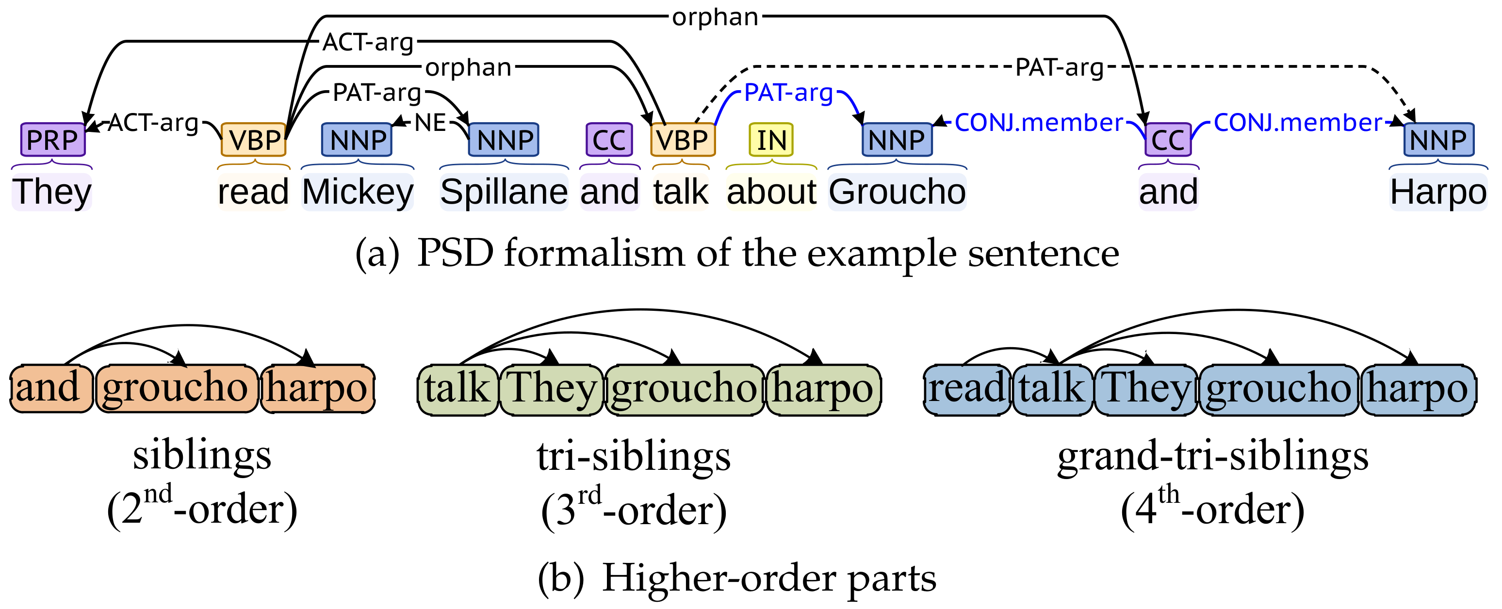Here is a straightforward example (as in Figure 1). For the sentence “They read Mickey Spillane and talk about Groucho and Harpo”, its semantic dependency representation is shown in Figure 1a; the higher-order parts that appear in this sentence are shown in Figure 1b. When considering the semantic dependency relationship between talk and Harpo (dotted edge), if we know (1) Groucho and Harpo are included in the second-order part (siblings) and (2) there is a dependency edge labeled PAT-arg between talk and Groucho (blue edges), it is obvious that there is also a dependency edge labeled PAT-arg between talk and Harpo.

Several semantic dependency parsers have been presented in recent years. Most of them are first-order parsers that utilize the information about first-order parts [10,11,12,13,14]; the rest are second-order parsers that utilize the information about second-order parts [8,15,16]. They have demonstrated that second-order information could bring significant accuracy gains in SDP. However, the second-order parts used in these second-order parsers are limited to specific types, including siblings, grandparent, and co-parents. Utilizing more types of higher-order parts (e.g. tri-siblings, great-grandparents, grand-tri-siblings, etc.) in SDP still remains under-explored. The reason for this issue is that modeling higher-order parts is non-trivial [8]. Higher-order parts have been exploited in syntactic dependency parsing [7,9,17,18,19]. However, algorithms for higher-order syntactic dependency parsing aim to generate a dependency tree rather than a dependency graph, therefore they are not applicable to SDP.

Graph neural networks (GNNs) have been demonstrated to be an effective tool for encoding higher-order information in many graph learning tasks [7,20]. GNNs aggregate higher-order information in a similar incremental manner: One GNN layer encodes information about immediate neighbors and K layers encode K-order neighborhoods (i.e., information about nodes at most K hops away).

This study aims to exploit GNNs’ powerful ability of representation learning in SDP. Inspired by the success of GNNs, we investigate using GNNs to encode higher-order information to improve the accuracy of SDP. Instead of encoding higher-order information of specific types of higher-order parts extracted from intermediate parsing graphs, we aggregate higher-order information by stacking multiple GNN layers. We extend the biaffine parser [12] and employ it as the vanilla parser to produce an initial adjacency matrix (close to gold) since there is no graph structure available during testing. Two GNN variants, Graph Convolutional Network (GCN) [21] and Graph Attention Network (GAT) [22], have been investigated in our model (GNNSDP: GNN-based Semantic Dependency Parser).

GNNSDP has been evaluated on the SemEval 2015 Task 18 dataset which covers three languages (Chinese, English, and Czech) and contains three semantic dependency formalisms (DM, PAS, and PSD). Compared to the previous best one, our parser yields 0.3% and 2.2% improvement in average labeled F1-score on English in-domain (ID) and out-of-domain (OOD) test sets, 2.6% improvement on Chinese ID test set, and 2.0% and 1.8% improvement on Czech ID and OOD test sets. Experimental results show that GNNSDP outperforms the previous state-of-the-art parser in three languages. In addition, GNNSDP shows greater advantage over the baseline in the longer sentence and PSD formalism (appearing linguistically most fine grained). To the best of our knowledge, this work is the first study to apply GNNs in semantic dependency parsing. Our code is publicly available at https://github.com/LiBinNLP/GNNSDP (accessed on 16 April 2022).

2. Related Work

In this section, the studies on higher-order syntactic dependency parsing, semantic dependency parsing, and GNNs will be summarized.

2.1. Higher-Order Syntactic Dependency Parsing

Higher-order parsing has received a lot of attention in the syntactic dependency parsing. McDonald and Pereira [23] presented a second-order parser which extended the maximum spanning tree parsing framework to incorporate second-order siblings parts. Carreras [17] presented a second-order parser which incorporated grand-parental relationships in the dependency structure. Koo and Collins [18] developed a third-order parser. They introduced grand-siblings and tri-siblings parts. Ma and Zhao [19] developed a forth-order parser which utilized grand-tri-siblings parts for fourth-order dependency parsing. Ji et al. [7] used GNNs to capture higher-order information for syntactic dependency parsing, which was closely related to our work. The core difference between their method and ours is that they integrated three types of high-order information (grandparent, grandchild, and siblings), and ours is not limited to any specific types of higher-order parts. Zhang et al. [9] presented a second-order TreeCRF extension to the biaffine parser.

Higher-order parts have been exploited in syntactic dependency parsing. However, approaches for higher-order syntactic dependency parsing aim to generate a dependency tree rather than a dependency graph. Therefore, they are not applicable to semantic dependency parsing.

2.2. Semantic Dependency Parsing

Several SDP models have been presented in recent years. Their parsing mechanisms are either transition based or graph based. Most of them are first-order parsers. Wang et al. [13] presented a neural transition-based parser, using a variant of the list-based arc-eager transition algorithm for dependency graph parsing. Lindemann et al. [24] developed a transition-based parser for Apply-Modify dependency parsing. They extended the stack-pointer model to predict transitions. Fernández-González and Gómez-Rodríguez [14] developed a transition-based parser, using the Pointer Network to choose a transition between Attach-p and Shift. More recently, there has been a predominance of purely graph-based SDP models. Dozat and Manning [12] extended the LSTM-based syntactic parser of Dozat et al. [25] to train on and generate SDG. Kurita and Søgaard [26] developed a reinforcement learning-based approach that iteratively applied the syntactic dependency parser to build a DAG structure sequentially. Jia et al. [27] presented a semi-supervised model based on the Conditional Random Field Autoencoder to learn a dependency graph parser. He and Choi [28] significantly improved the performance by introducing contextual string embeddings (called Flair).

Higher-order SDP has received less attention. Martins et al. [15] developed a second-order parser which employed a feature-rich linear model to incorporate first and second-order parts (arcs, siblings, grandparent, and co-parents). The $A{D}^3$ algorithm was employed for approximate decoding. Cao et al. [16] presented a quasi-second-order parser and used a dynamic programming algorithm (called Maximum Subgraph) for exact decoding. Wang et al. [8] extended the parser [12] and managed to add the information about three types of second-order parts (siblings, grandparent, and co-parents) for score computation and then applied either mean-field variational inference or loopy belief propagation for approximate decoding.

These second-order parsers demonstrated that second-order information could bring significant accuracy gains in SDP. However, the second-order parts used in these second-order parsers are limited to specific types, including siblings, grandparent, and co-parents. Utilizing more types of higher-order parts (e.g., tri-siblings, great-grandparent, grand-tri-siblings, etc.) in SDP still remains under-explored. The reason for this issue is that modeling higher-order parts is non-trivial [8].

2.3. Graph Neural Networks

Recent years have witnessed great success from GNNs [21,22,29] in graph learning. GNNs follow a message-passing mechanism, where the node embedding is obtained by aggregating and transforming the embeddings of its neighbors. Due to the powerful ability to learn effective representations of graphs, GNNs have been applied to various downstream tasks including node classification, link prediction, and graph classification.

Two main families of GNNs have been proposed, i.e., spectral methods and spatial methods. The first family learns node representation based on graph spectral theory [21,30,31]. The second family defines graph convolutions in the spatial domain as aggregating and transforming local information [22,29]. GCNs [21] is a spectral-based method, which learns node representation based on graph spectral theory. GAT [22] is a spatial-based method, which introduces the multi-head attention mechanism to learn different attention scores for neighbors when aggregating information.

GNNs have been demonstrated to be an effective tool for encoding higher-order information in many graph learning tasks [7,20]. Marcheggiani and Titov [20] utilized GNNs to capture higher-order information from the syntactic dependency tree for semantic role labeling. Ji et al. [7] utilized GNNs to encode specific types of higher-order parts for syntactic dependency parsing.

Inspired by the success of GNNs, we investigate using GNNs to encode higher-order information for improving semantic dependency parsing.

3. GNN-Based Semantic Dependency Parser

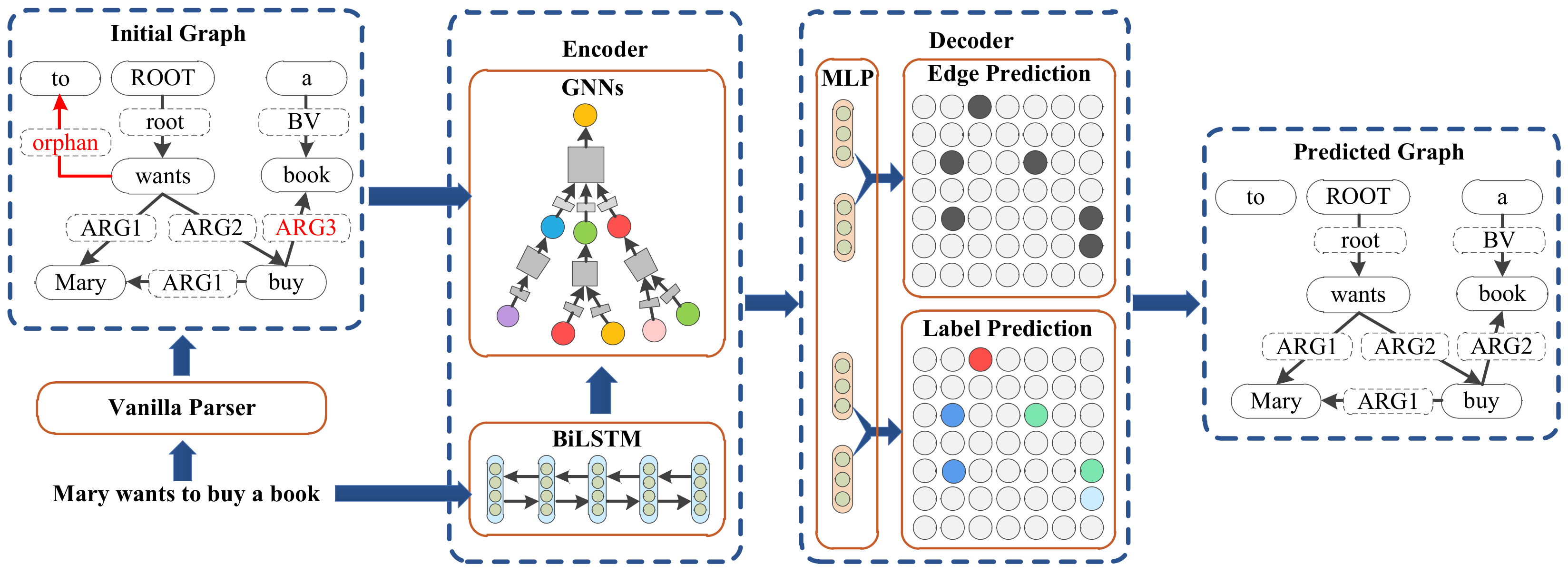
GNNSDP is a parser that extends the biaffine parser [12]. An overview of GNNSDP is shown in Figure 2. Given sentence s with n words $[w_1,w_2,\dots ,w_n]$, there are three steps to parse it as an SDG. Firstly, the sentence will be parsed with a vanilla SDP parser, producing an initial SDG. Secondly, the contextualized word representations output by long short-term memory (BiLSTM) and adjacency matrix obtained from the initial SDG will be fed into the GNN encoder to obtain node representations which contain higher-order information. Finally, Multi-Layer Perceptron (MLP) will be used to get the hidden state representation, and then decoded by the biaffine classifier to predict edge and label.

3.1. Vanilla Parser

We use the biaffine parser [12] as the vanilla parser. Sentence s will be parsed by the vanilla parser to obtain the initial adjacency matrix.

$$(\tilde{A},\tilde{G})=VanillaParser(W,F)$$

(1)

where $\tilde{A}$ is the initial adjacency matrix; $\tilde{G}$ is the initial SDG; W denotes n words and F denotes features of words.

3.2. Embeddings

Word embeddings and feature embeddings are used to represent the embedding of each token in GNNSDP.

3.2.1. Word Embeddings

Pretrained word embeddings of three languages are downloaded from the internet:

• For English, the 100-dimension English word embeddings from GloVe [32] are used.
• For Chinese, the 300-dimension Chinese word embeddings from SGNS [33] are used.
• For Czech, the 300-dimension Czech word embeddings from fasttext [34] are used.

3.2.2. Feature Embeddings

Four types of features are used in GNNSDP. The dimension of each feature embedding is denoted as d ($d=100$):

• Part-of-speech (POS) tag embeddings: POS tag embeddings $E^{\left(pos\right)}$ are randomly generated. $E^{\left(pos\right)}\in R^{n\times d}$, where n is the number of POS tags.
• Lemma embeddings: A lemma is the base form of a word; lemma embeddings $E^{\left(lemma\right)}$ are also randomly generated. $E^{\left(lemma\right)}\in R^{l\times d}$, where l is the number of lemmas. Lemmas that occurred seven times or more are included in the lemma embedding matrix.
• Character embeddings: Character embeddings summarize the information of characters in each token, which are generated using a one-layer unidirectional LSTM (CharLSTM) that convolves over three character embeddings at a time, whose end state is linearly transformed to be d-dimensional.
• Bidirectional Encoder Representation from Transformer (BERT) embeddings: BERT embeddings are extracted from the pretrained BERT model.

3.3. Encoder

We concatenate word embeddings and feature embeddings, and feed them into a BiLSTM to obtain contextualized representations.

Specifically, BiLSTM is a sequence processing model that consists of two reversed unidirectional LSTM networks: One taking the input in a forward direction to capture forward information, and another in a backward direction to capture backward information. BiLSTM can integrate both forward and backward information by concatenating bidirectional information.

$$x_i=e_i^{\left(word\right)}\oplus e_i^{\left(feat\right)}$$

(2)

$$\overrightarrow{o_i}=LST{M}^{\left(forward\right)}\left(x_i\right)$$

(3)

$$\overleftarrow{o_i}=LST{M}^{\left(backward\right)}\left(x_i\right)$$

(4)

$$o_i=\overrightarrow{o_i}\oplus \overleftarrow{o_i}$$

(5)

where $x_i$ is the concatenation (⊕) of the word embeddings and feature embeddings of word $w_i$, X represents $[x_1,x_2,\dots ,x_n]$. $O=[o_1,o_2,\dots ,o_n]$ is the contextualized representations of sequence X.

Then we employ K-layer GNNs to capture higher-order information by aggregating the representation of K-order neighborhoods. The node embedding matrix $R^{\left(k\right)}$ in the kth-layer is computed as Equation (6):

$$R^{\left(k\right)}=GNNLaye{r}^{(k-1)}(R^{(k-1)},\tilde{A})$$

(6)

When the GNNLayer is implemented in the GCN, the representation $r_i^{\left(k\right)}$ of node i in the kth layer is computed as Equation (7)

$$r_i^{\left(k\right)}=\sigma \left(W\sum _{j\in N\left(i\right)}{r}_j^{(k-1)}+B{r}_i^{(k-1)}\right)$$

(7)

where W and B are parameter matrices; $N\left(i\right)$ are neighbors of node i; $\sigma$ is the active function (ReLU is used); $r_i^{\left(0\right)}=o_i$.

When GNNLayer is implemented in GAT, $r_i^{\left(k\right)}$ is computed as Equation (8):

$$r_i^{\left(k\right)}=\sigma \left(W\sum _{j\in N\left(i\right)}{a}_{ij}^{\left(m\right)(k-1)}{r}_j^{(k-1)}+B{r}_i^{(k-1)}\right)$$

(8)

where $a_{ij}^{\left(m\right)(k-1)}$ is the attention coefficient of node i to its neighbour j in attention head m at the $(k-1)$th layer.

While higher-order information is important, GNNs would suffer from the over-smoothing problem when the number of layer is excessive. Therefore we stack three layers with the past experience.

3.4. Decoder

The decoder has two modules: The edge existence prediction module and the edge label prediction module. For each of the two modules, we use MLP to split the final node representation $R=[r_1,r_2,\dots ,r_n]$ into two parts—a head representation, and a dependent representation, as shown in Equations (9)–(12):

$$h_i^{(edge-head)}=ML{P}^{(edge-head)}\left(r_i\right)$$

(9)

$$h_i^{(label-head)}=ML{P}^{(label-head)}\left(r_i\right)$$

(10)

$$h_i^{(edge-dep)}=ML{P}^{(edge-dep)}\left(r_i\right)$$

(11)

$$h_i^{(label-dep)}=ML{P}^{(label-dep)}\left(r_i\right)$$

(12)

We can then use two biaffine classifiers (as Equation (13)), which are generalizations of linear classifiers to include multiplicative interactions between two vectors—to predict edges and labels, as Equations (14) and (15):

$$Biaff(x_1,x_2)=x_1^{T}U{x}_2+W(x_1\oplus x_2)+b$$

(13)

$$s_{i,j}^{\left(edge\right)}=Biaf{f}^{\left(edge\right)}(h_i^{(edge-dep)},h_j^{(edge-head)})$$

(14)

$$s_{i,j}^{\left(label\right)}=Biaf{f}^{\left(label\right)}(h_i^{(label-dep)},h_j^{(label-head)})$$

(15)

where $s_{i,j}^{\left(edge\right)}$ and $s_{i,j}^{\left(label\right)}$ are scores of edge existence and edge label between words $w_i$ and $w_j$. U, W, and b are learned parameters of the biaffine classifier. For the edge existence prediction module, U will be $(d\times 1\times d)$-dimensional, so that the $s_{i,j}^{\left(edge\right)}$ will be a scalar. For edge label prediction, if the parser is unlabeled, U will be $(d\times 1\times d)$-dimensional, so that the $s_{i,j}^{\left(label\right)}$ will be a scalar. If the parser is labeled, U will be $(d\times c\times d)$-dimensional, where c is the number of labels, so that the $s_{i,j}^{\left(label\right)}$ is a vector that represents the probability distributions of each label.

The unlabeled parser scores each edge between pairs of words in the sentence—these scores can be decoded into a graph by keeping only edges that received a positive score. The labeled parser scores every label for each pair of words, so we simply assign each predicted edge its highest-scoring label and discard the rest.

$${\widehat{y}}_{i,j}^{\left(edge\right)}=\{s_{i,j}^{\left(edge\right)}>0\}$$

(16)

$${\widehat{y}}_{i,j}^{\left(label\right)}=arg max{s}_{i,j}^{\left(label\right)}$$

(17)

3.5. Learning

We can train the model by summing the losses from the two modules, back propagating the error to the parser. The cross entropy function is used as as the loss function, which is computed as Equation (18):

$$CE(p,q)=-\sum _{x}p\left(x\right)logq\left(x\right)$$

(18)

The loss functions of the edge existence prediction module and the edge label prediction module are defined as:

$${\mathcal{L}}^{\left(edge\right)}\left({\theta }_1\right)=CE({\widehat{y}}_{i,j}^{\left(edge\right)},y_{i,j}^{\left(edge\right)})$$

(19)

$${\mathcal{L}}^{\left(label\right)}\left({\theta }_2\right)=CE({\widehat{y}}_{i,j}^{\left(label\right)},y_{i,j}^{\left(label\right)})$$

(20)

where ${\theta }_1$ and ${\theta }_2$ are the parameters of two modules.

Then the adaptive moment estimation (Adam) method is used to optimize the summed loss function $\mathcal{L}$:

$$\mathcal{L}=\lambda {\mathcal{L}}^{\left(edge\right)}+(1-\lambda ){\mathcal{L}}^{\left(label\right)}$$

(21)

where $\lambda$ is a tunable interpolation constant $\lambda \in (0,1)$.

4. Experiments

In this section, the dataset, hyper-parameters, and experimental results are shown as follows.

4.1. Dataset

In order to test the proposed approach, we conducted experiments on the SemEval 2015 Task 18 dataset [35], which covers three languages (English, Chinese, and Czech) and contains three different formalisms (DELPH-IN MRS (DM) [36], Predicate-Argument Structure (PAS) [37], and Prague Semantic Dependencies (PSD) [38]). For English, three formalisms (DM, PAS, and PSD) are all available; for Chinese, only PAS formalism is available; for Czech, only PSD formalism is available.

The dataset split of three languages is shown as

Table 1. The number of sentences contained in each divided dataset of three languages. Only the in-domain test set is available for Chinese; the in-domain and out-of-domain test sets are available for English and Czech.

Language	Train Set	Development Set	Test Set
			ID	OOD
English (DM/PAS/PSD)	33,964	1692	1410	1849
Chinese (PAS)	25,336	3000	8976	-
Czech (PSD)	39,057	3000	1670	316

. For English, we use the same dataset split as in previous approaches [10,39], with 33,964 training sentences from Sections 00-19 of the Wall Street Journal corpus [40], 1692 development sentences from Section 20, 1410 sentences from Section 21 as in-domain (ID) test data, and 1849 sentences sampled from the Brown Corpus [41] as the out-of-domain (OOD) test data. For Chinese, we use the top 3000 sentences as the development data, the remaining 25,336 sentences as the training data, and 8976 sentences as the ID test data. For Czech, we use the top 3000 sentences as the development data, the remaining 39,057 sentences as the training data, 1670 sentences as the ID test data, and 316 sentences as the OOD test data.

For the evaluation, we use the evaluation script used in Wang et al. [8], reporting labeled F-measure scores (LF1) (including ROOT arcs) on the ID and OOD test sets for each formalism as well as the macro-average over the three of them.

4.2. Experimental Environments

The main hardware and software used in our experimental environments are shown as

Table 2. Hardware and software used in our experimental environments.

Hardware/Software	Value
CPU	Intel Xeon(R) Silver 4216 @ 2.1GHz(16-core)
Memory	128 GB
GPU	NVIDIA RTX 2080Ti(11G)
Python	3.6.1
Pytorch	1.9.0
Anaconda	4.8.3
CUDA	11.0
IDE	Pycharm

. GPU is utilized to do the computation of neural networks, to speed up the process of training and prediction.

4.3. Hyper-Parameters

The hyper-parameter configuration for our final system is given in

Table 3. Final hyper-parameter configuration.

Layer	Hyper-Parameter	Value
Word Embedding	English	100
	Chinese/Czech	300
Feature Embedding	POS/Lemma/Char/BERT	100
LSTM	layers	3
	hidden size	400
	dropout	0.33
GNN	GCN layers/GAT heads	3
	GAT $\alpha$	0.2
	GCN/GAT dropout	0.33
MLP	edge-head/label-head hidden size	600
	edge-dep/label-dep hidden size	600
Trainer	optimizer	Adam
	learning rate	1 $\times {10}^{-2}$
	Adam (${\beta }_1$, ${\beta }_2$)	(0.95, 0.95)
	decay rate	0.75
	decay step length	5000
	$\lambda$	0.1

. Following Wang et al. [8], we use Adam to optimize our model, annealing the learning rate by 0.5 for every 10,000 steps, and switch the optimizer to AMSGrad after 5000 steps without improvement. We train the model for 100,000 iterations with batch sizes of 6000 tokens and terminate the training early after 10,000 iterations with no improvement on the development set.

4.4. Baseline Approaches

We compare GNNSDP with previous state-of-the-art parsers in

Table 4. Comparison of labeled F1 scores achieved by our model and previous state-of-the-art in the English dataset. The bold numbers indicate the current best scores. The F1 scores of baseline and our models are averaged over five runs. ID denotes the in-domain (WSJ) test set and OOD denotes the out-of-domain (Brown) test set. +Char, +Lemma, +BERT, and +Flair mean augmenting the token embeddings with character-level, lemma embeddings, BERT embeddings, and Flair embeddings. Semi-SDP only shows the full-supervised result on DM formalism.

	English
Models	DM		PAS		PSD		Avg
	ID	OOD	ID	OOD	ID	OOD	ID	OOD
Peking [10]	89.1	81.8	91.3	87.2	75.7	73.3	85.3	80.8
Lisbon [39]	88.2	81.8	90.9	86.9	76.4	74.8	85.2	81.2
PTS17 [11]: Basic	89.4	84.5	92.2	88.3	77.6	75.3	86.4	82.7
PTS17 [11]: Basic	90.4	85.3	92.7	89.0	78.5	76.4	87.2	83.6
WCGL [13]	90.3	84.9	91.7	87.6	78.6	75.9	86.9	82.8
D&M [12]: Basic	91.4	86.9	93.9	90.8	79.1	77.5	88.1	85.0
MF [8]: Basic	93.0	88.4	94.3	91.5	80.9	78.9	89.4	86.3
LBP [8]: Basic	92.9	88.4	94.3	91.5	81.0	78.8	89.4	86.2
Lindemann et al. [44]: Basic	91.2	85.7	92.2	88.0	78.9	76.2	87.4	83.3
SemPointer [14]: Basic	92.5	87.7	94.2	91.0	81.0	78.7	89.2	85.8
GNNSDP(GCN): Basic	93.3	88.0	94.8	91.1	85.6	83.6	91.2	87.6
GNNSDP(GAT): Basic	93.0	87.9	94.8	91.6	85.4	83.3	91.1	87.6
D&M [12]: +Char+Lemma	93.7	88.9	93.9	90.6	81.0	79.4	89.5	86.3
MF [8]: +Char+Lemma	94.0	89.7	94.1	91.3	81.4	79.6	89.8	86.9
LBP [8]: +Char+Lemma	93.9	89.5	94.2	91.3	81.4	79.5	89.8	86.8
Jia et al. [27]: +Lemma	93.6	89.1	-	-	-	-	-	-
SemPointer [14]: +Char+Lemma	93.9	89.6	94.2	91.2	81.8	79.8	90.0	86.9
GNNSDP(GCN): +Char+Lemma	94.2	90.1	94.9	91.4	86.4	84.9	91.8	88.8
GNNSDP(GAT): +Char+Lemma	94.4	89.9	95.0	91.8	86.2	84.6	91.9	88.8
Lindemann et al. [44]: +BERTlarge	94.1	90.5	94.7	92.8	82.1	81.6	90.3	88.3
Lindemann et al. [24]: +BERTlarge	93.9	90.4	94.7	92.7	81.9	81.6	90.2	88.2
SemPointer [14]: +Char+Lemma+BERTbase	94.4	91.0	95.1	93.4	82.6	82.0	90.7	88.8
He et al. [28]: +Char+Lemma+BERTbase+Flair	94.6	90.8	96.1	94.4	86.8	79.5	92.5	88.2
GNNSDP(GCN): +Char+Lemma+BERTbase	95.1	91.1	95.7	93.2	87.7	87.3	92.8	90.5
GNNSDP(GAT): +Char+Lemma+BERTbase	95.3	91.9	96.0	94.3	87.0	86.7	92.8	91.0

and Table 6. Turku is from Kanerva et al. [42]. Riga is from Barzdins et al. [43]. Peking is a hybrid model from Du et al. [10]. Lisbon is from Almeida and Martins [39]. WCGL [13] is a neural transition-based model. PTS17 is proposed by Peng et al. [11] and Basic is single task parsing, while Freda3 is a multitask parser across three formalisms. D&M [12] is a first-order graph-based model. MF and LBP [8] are a second-order model using mean field variational inference or loopy belief propagation. Lindemann et al. [44] and Lindemann et al. [24] are a compositional semantic parser for SDP and abstract meaning representation. SemPointer [14] is a transition-based model using the Pointer Network. Jia et al. [27] is a semi-supervised parser, only the full-supervised result on DM formalism is shown in their paper. He and Choi [28] uses not only BERT but also contextual string embeddings (called Flair).

4.5. Experimental Results

We group SDP models into three blocks depending on the embeddings provided to the models: (1) just basic pre-trained word embeddings and POS tag embeddings (Basic), (2) character and pre-trained lemma embeddings augmentation (+Char+Lemma), and (3) pre-trained BERT embedding augmentation (+Char+Lemma+BERT).

4.5.1. Results on English

Table 4 presents the comparison of GNNSDP and previous approaches on the test sets of the SemEval 2015 Task 18 English dataset. From the results, we have the following observations:

• In the basic settings, GNNSDP achieves 1.8 and 1.3 averaged LF1 improvements on the ID and OOD test set over the previous best parsers.
• Adding both the character-level and the lemma embeddings, most models improve performance quite a bit generally. GNNSDP leads to 1.9 and 1.9 averaged LF1 improvements over the previous best parsers on the ID and OOD test sets.
• Adding BERT embeddings pushes performance even higher generally. GNNSDP outperforms the previous best parsers by 0.3 and 2.2 average LF1 improvements on the ID and OOD test sets, respectively.
• GNNSDP makes significant improvements on the PSD formalism, with 4.6 and 4.7 LF1 improvements in the basic settings, 4.6 and 5.1 LF1 improvements when character-level and lemma embeddings are added, 0.9 and 5.3 LF1 improvements when BERT embeddings are added on the ID and OOD test sets, respectively.
• The LF1 scores of all parsers on the PSD is lower than the other two formalisms.

  Table 5. Contrastive statistics of three semantic formalisms.

  	DM		PAS		PSD
  	ID	OOD	ID	OOD	ID	OOD
  # labels	59	47	42	41	91	74
  # frames	297	172	-	-	5426	1208

  shows part of contrastive statistics of three formalisms. We have noticed that the PSD formalism appears linguistically most fine-grained because it contains the most semantic labels and frames [35]. This makes PSD more challenging to predict. However, GNNSDP performs better than other first-order and second-order parsers, suggesting that higher-order information is beneficial for improving SDP.
• The performances of GNNSDP(GCN) and GNNSDP(GAT) are close in three embedding settings, demonstrating that both GCN and GAT are capable of capturing higher-order information.

4.5.2. Results on Chinese and Czech

Table 6. Comparison of labeled F1 scores achieved by our model and previous state-of-the-art on Chinese and Czech datasets. The bold numbers indicate the current best scores. The results of D&M on Chinese and Czech are not reported in their paper; therefore, we reproduce it. The F1 scores of baseline and our models are averaged over five runs. Only the PAS formalism and in-domain test set is available for Chinese; the PSD formalism, in-domain, and out-of-domain test sets are available for Czech.

	Chinese	Czech
Models	PAS	PSD
	ID	ID	OOD
Turku [42]	79.6	75.3	63.7
Riga [43]	82.5	75.3	61.3
Peking [10]	83.4	78.5	64.4
Lisbon [39]	82.0	79.3	63.5
D&M [12]: Basic	87.4	86.9	77.8
GNNSDP(GCN): Basic	88.3	88.2	79.1
GNNSDP(GAT): Basic	88.0	87.8	78.9
D&M [12]: +Char+Lemma	87.8	87.6	78.9
GNNSDP(GCN): +Char+Lemma	88.5	88.8	80.2
GNNSDP(GAT): +Char+Lemma	88.3	88.9	80.2
GNNSDP(GCN): +Char+Lemma+BERTbase	90.1	89.6	80.7
GNNSDP(GAT): +Char+Lemma+BERTbase	90.4	89.3	80.4

shows the comparison of GNNSDP and previous studies on the SemEval 2015 Task 18 Chinese and Czech datasets. From the results, we have observed that:

• GNNSDP(GCN) and GNNSDP(GAT) outperform the previous parsers on Chinese and Czech.
• The LF1 scores of GNNSDP(GCN) and GNNSDP(GAT) are relatively close on Chinese and Czech.

In summary, GNNSDP outperforms the previous state-of-the-art parser in three languages and three semantic dependency formalisms. Outstanding performances of GNNSDP have demonstrated that higher-order information can bring considerable accuracy gains in SDP. In addition, GNNs are capable of capturing higher-order information.

5. Experimental Analysis

In this section, we analyse the experimental results from three perspectives, including performance on different sentence length, ablation study, and case study.

5.1. Performance on Different Sentence Length

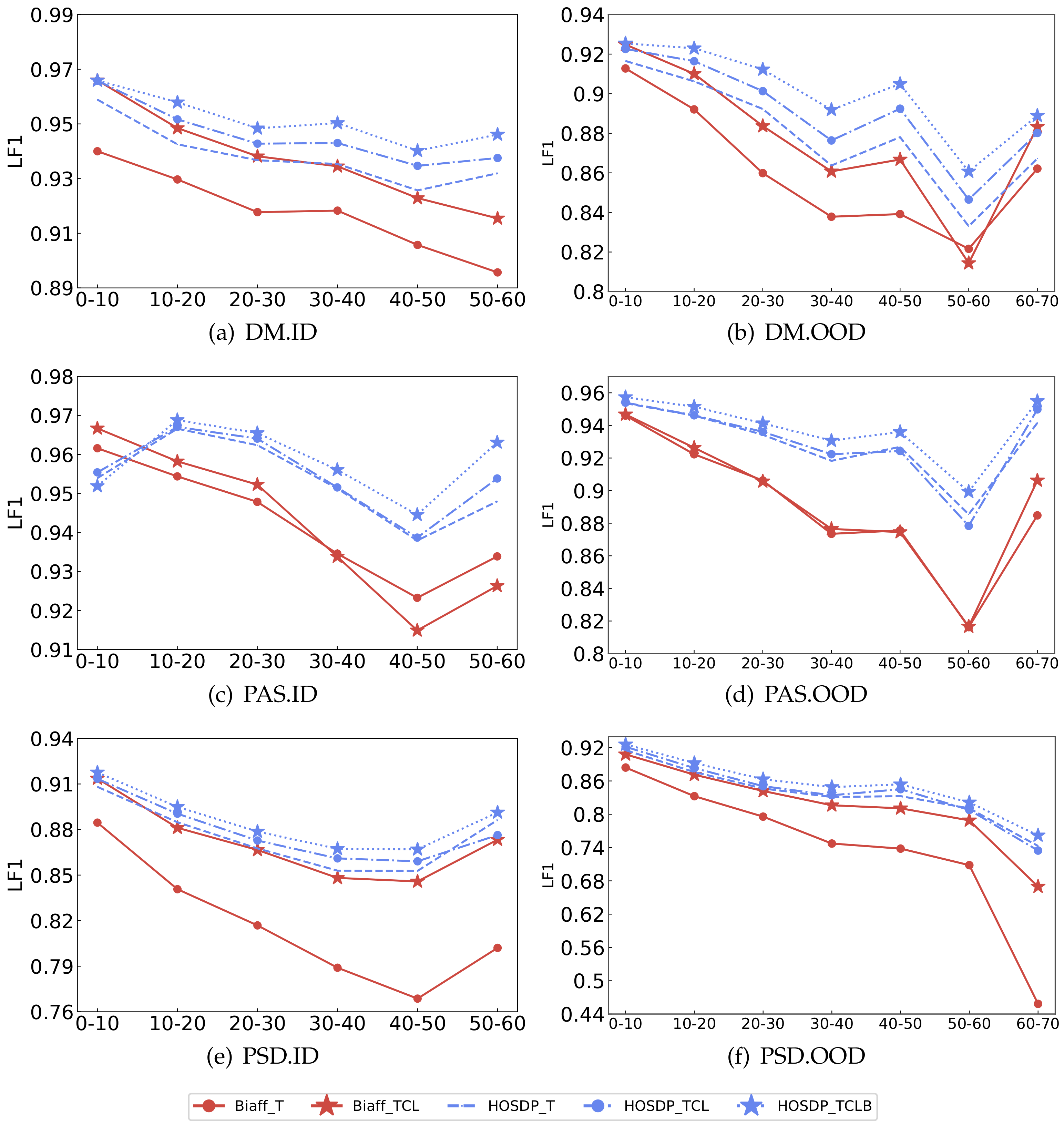
We want to study the impact of sentence lengths. The ID and OOD test sets of the three formalisms are split with 10 tokens range. The ID test set has six groups and OOD has seven groups. GNNSDP(GCN) and biaffine parser are evaluated on them. The results for different groups are shown in Figure 3.

The results show that GNNSDP outperforms the biaffine parser on different groups with the same embedding settings, except for being slightly lower on the first group (0–10 tokens) on ID test set of PAS formalism. Furthermore, GNNSDP that only uses POS tag embeddings outperforms the biaffine parser that uses POS tag, character-level, and lemma embeddings when sentences get longer, especially when sentences are longer than 30. It turns out that higher-order information is favorable for longer sentences since higher-order dependency relationships are more prevalent in longer sentences.

5.2. Ablation Study

We investigate how the number of GNN layers affects the performance of our parser. We train and test the GNNSDP(GCN) in PSD formalism datasets of English and Czech. The number of GCN layers increases from 1 to 3.

Table 7. LF1 scores of GNNSDP with different GNN layers on ID and OOD test set of Chinese and Czech. The bold numbers indicate the current best scores.

	English		Czech
Models	PSD		PSD
	ID	OOD	ID	OOD
D&M [12]	79.1	77.5	86.9	77.8
GNNSDP(GCN): 1-layer	83.4	81.9	87.7	78.6
GNNSDP(GCN): 2-layers	84.2	82.6	88.0	78.6
GNNSDP(GCN): 3-layers	85.6	83.6	88.2	79.1

shows the results of GNNSDP(GCN) with different numbers of GCN layers in basic embedding settings. From the results, we can see that:

• GNNSDP(GCN) with only one GCN layer still performs better than the biaffine parser, demonstrating that higher-order information is beneficial for improving SDP.
• The performance of GNNSDP(GCN) is gradually improved when the number of GCN layers is increased, demonstrating that stacking more GNN layers is able to capture better higher-order information.

5.3. Case Study

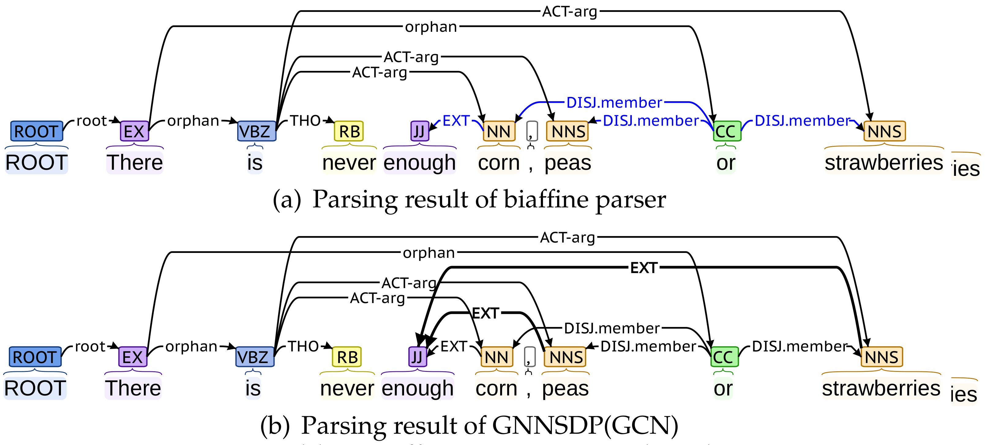
We provide a parsing example to show why GNNSDP benefits from higher-order information. Figure 4 shows the parsing results of the biaffine parser (Figure 4a) and GNNSDP(GCN) (Figure 4b) for the English sentence (sent_id = 40504035, in OOD of PSD formalism) “There is never enough corn, peas or strawberries”. Both parsers are trained in the basic embedding settings.

In the gold annotation, three words corn, peas, and strawberries are three members of the disjunctive word or. In addition, the word enough has three dependency edges labeled EXT with them. In the results of the biaffine parser, only the dependency edge between enough and corn is identified; the remaining two are not. In GNNSDP(GCN), given the initial SDG predicted by the biaffine parser, the words corn, peas, and strawberries aggregate the higher-order information of or and is (first-order), there (second-order), and ROOT (third-order). The word enough aggregates the higher-order information of the corn (first-order), is and or (second-order), there (third-order), and ROOT (fourth-order). The dependent word enough and three head words corn, peas, and strawberries aggregate information of four common words (ROOT, There, is and or). Therefore, the representations of them with higher-order information bring more evidence into decoders’ final decisions. As a result, it is effortless for GNNSDP to identify that there are also two dependency edges labeled EXT between the dependent word enough and the head words peas and strawberries.

6. Conclusions

This paper aims to exploit GNNs’ powerful ability of representation learning in SDP. GNNs are utilized to encode higher-order information to improve the accuracy of semantic dependency parsing. Experiments are conducted on the SemEval 2015 Task 18 dataset in three languages (Chinese, English, and Czech). Compared to the previous state-of-the-art parser, our parser yields 0.3% and 2.2% improvement in the average labeled F1-score on English in-domain (ID) and out-of-domain (OOD) test sets, 2.6% improvement on Chinese ID test set, and 2.0% and 1.8% improvement on the Czech ID and OOD test sets. Experimental results show that our parser outperforms the previous best one on the SemEval 2015 Task 18 dataset in three languages. In addition, our parser shows greater advantage in longer sentence and complex semantic formalism. Outstanding performances of our parser demonstrates that higher-order information encoded by GNNs is exceedingly beneficial for improving SDP.

Despite that significant improvement has been made, the initial graph structure output by the vanilla parser may be noisy, resulting in a performance penalty to some extent. In the future, we would like to apply graph structure learning models to jointly learn graph structure and graph representation, rather than depending on the initial dependency graph output by the vanilla parser.