
The Application of Satellite Image Analysis in Oil Spill Detection


Abstract
:1. Introduction
- -
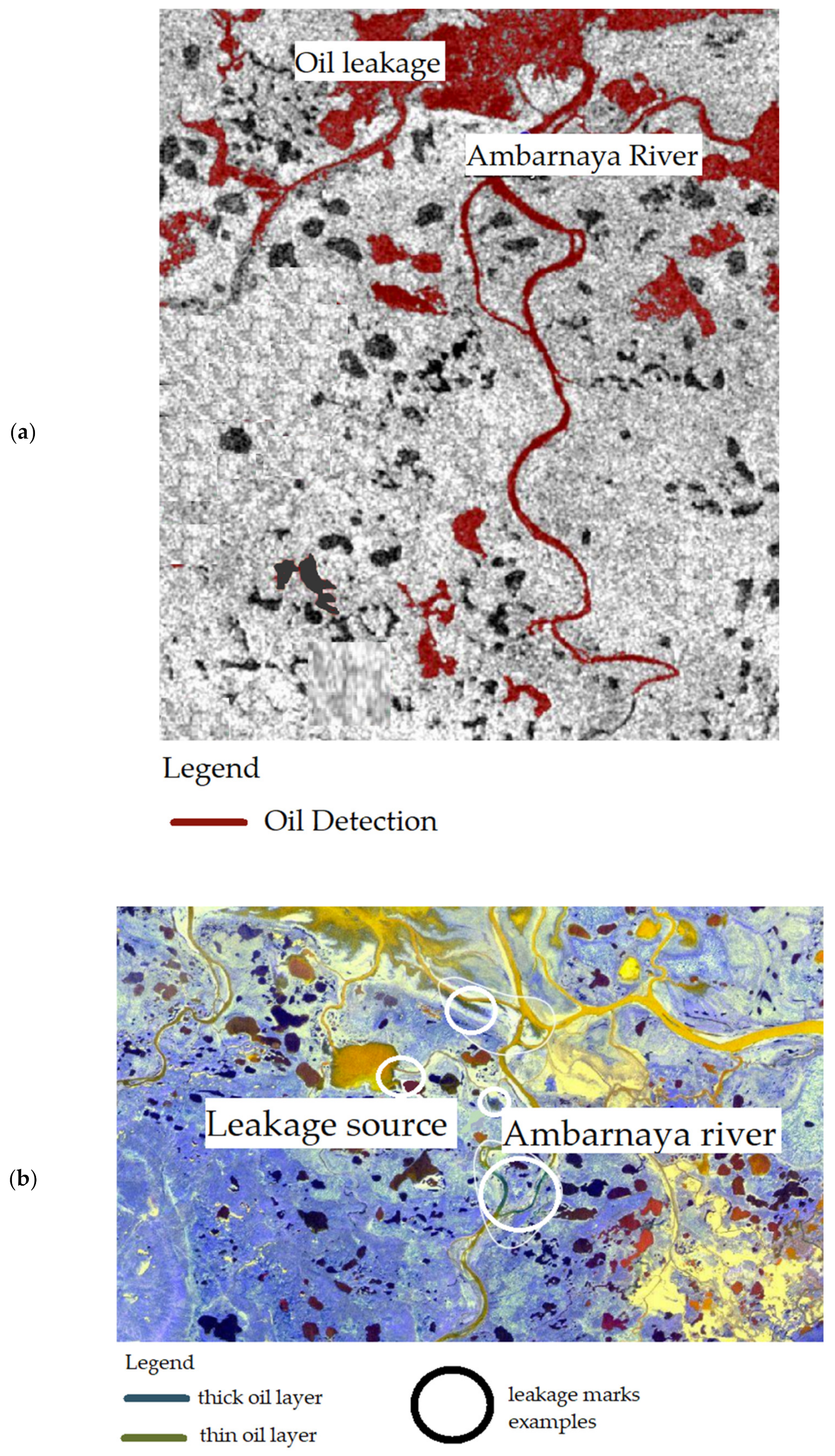
- conduct an analysis of oil spills in rivers,
- -
- group data for long- and short-term analysis,
- -
- select the appropriate classes according to the remote sensing device,
- -
- propose a practical method for monitoring oil spills.
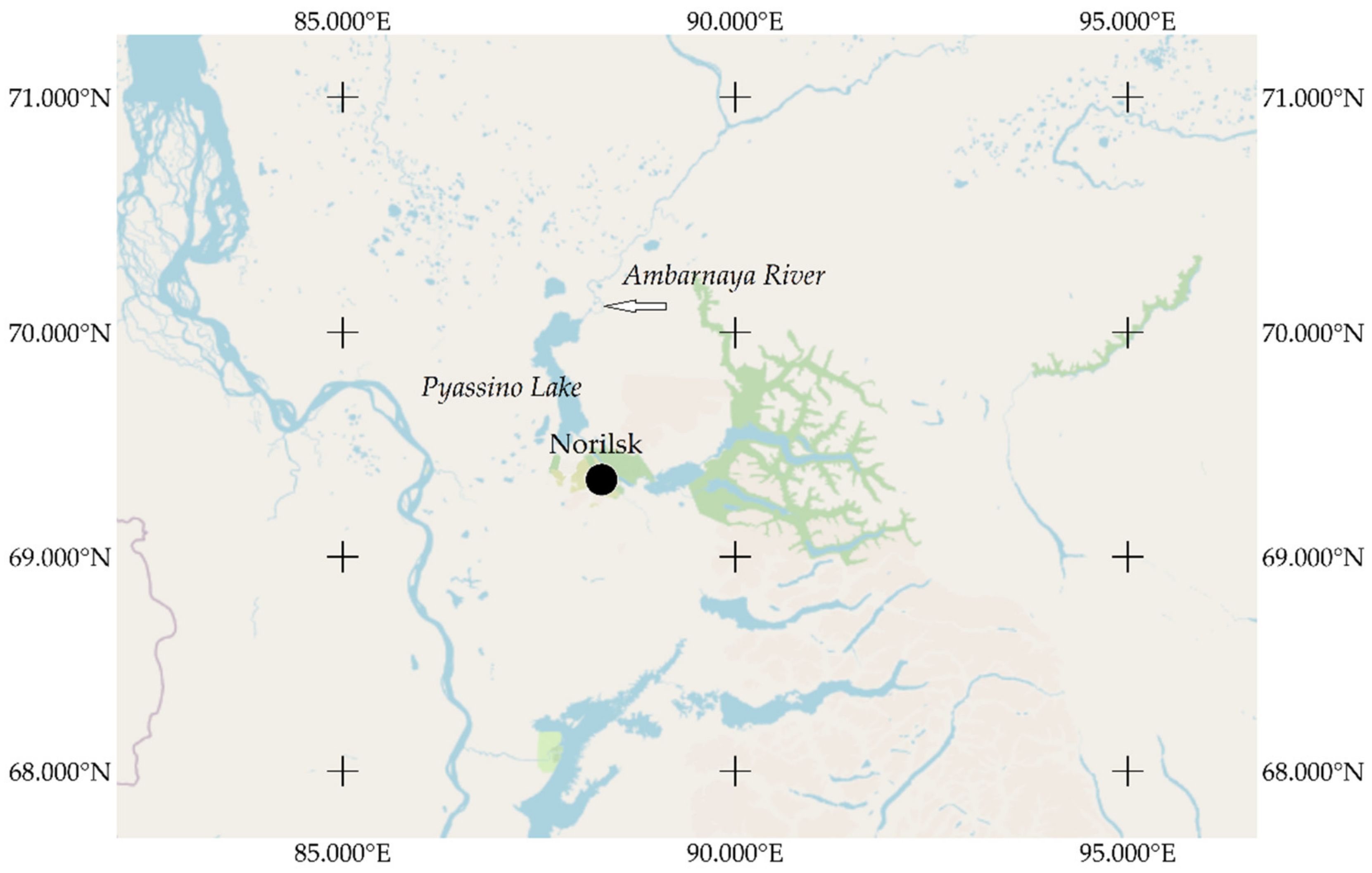
2. Materials and Methods
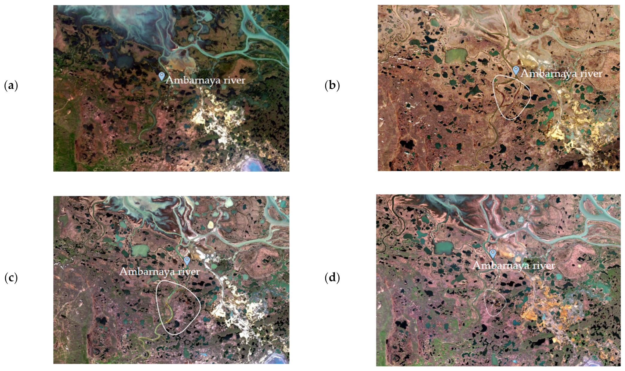
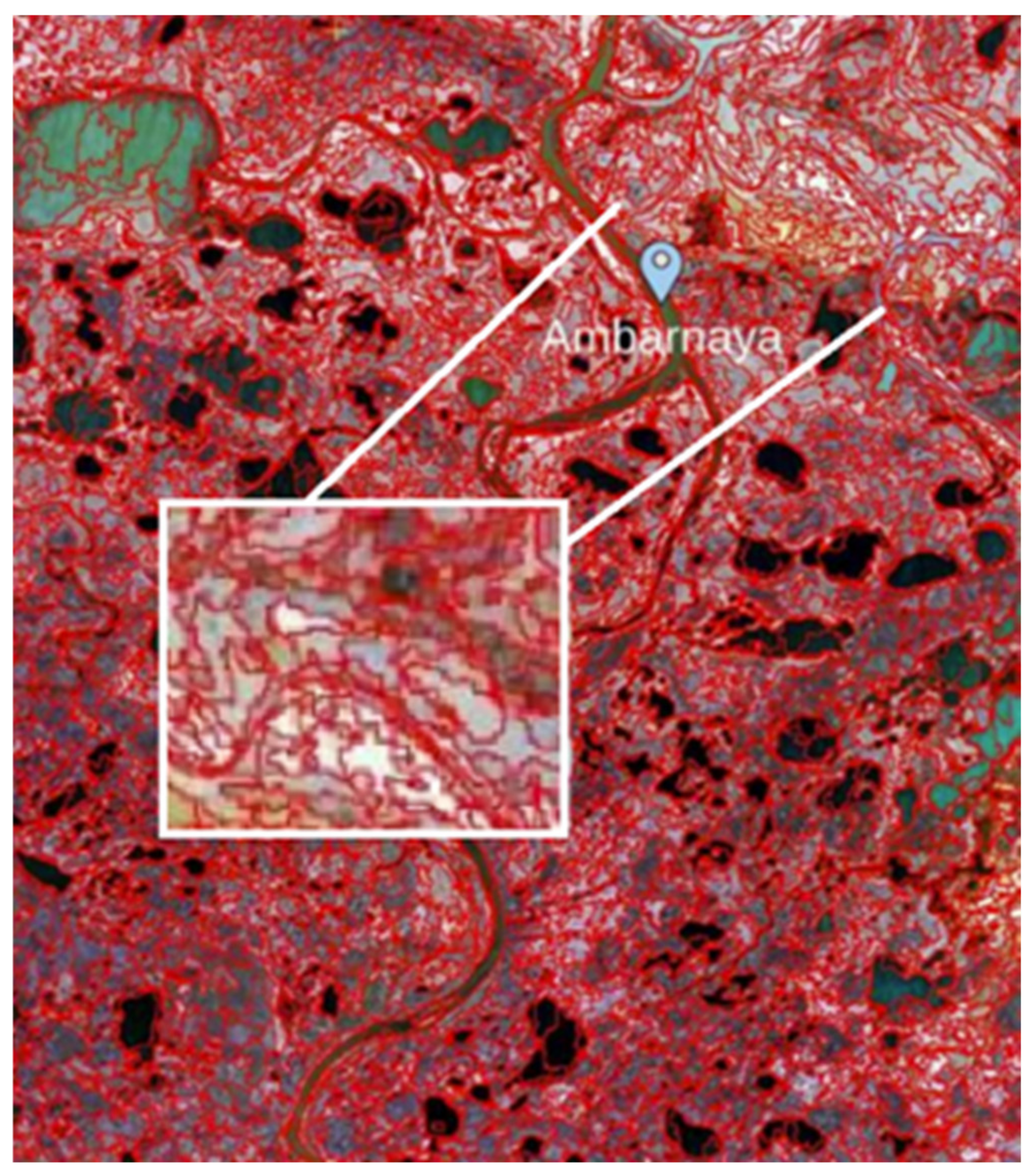
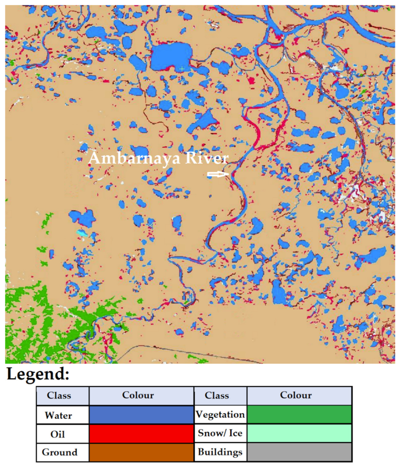
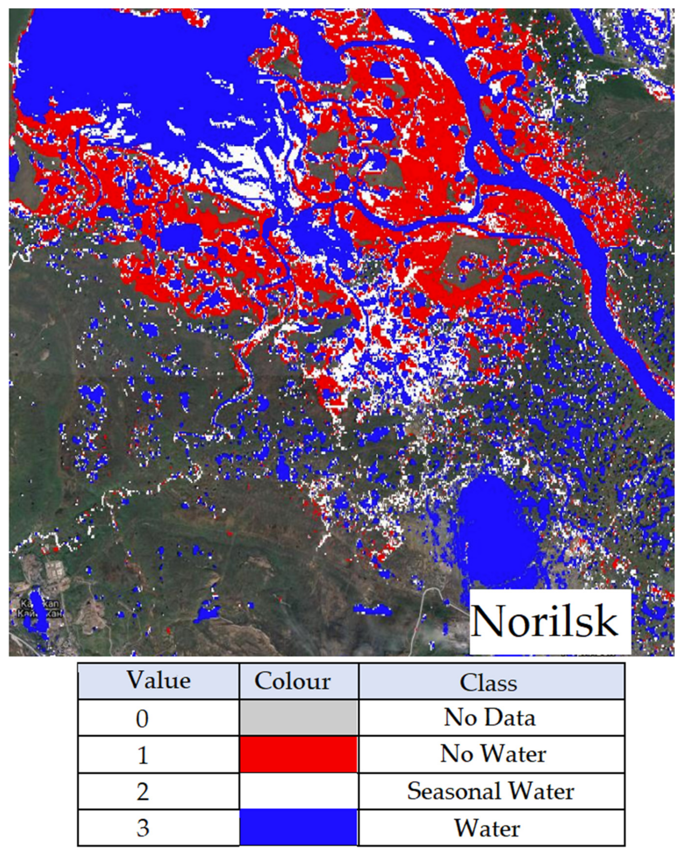
2.1. Study Site and Problem Description
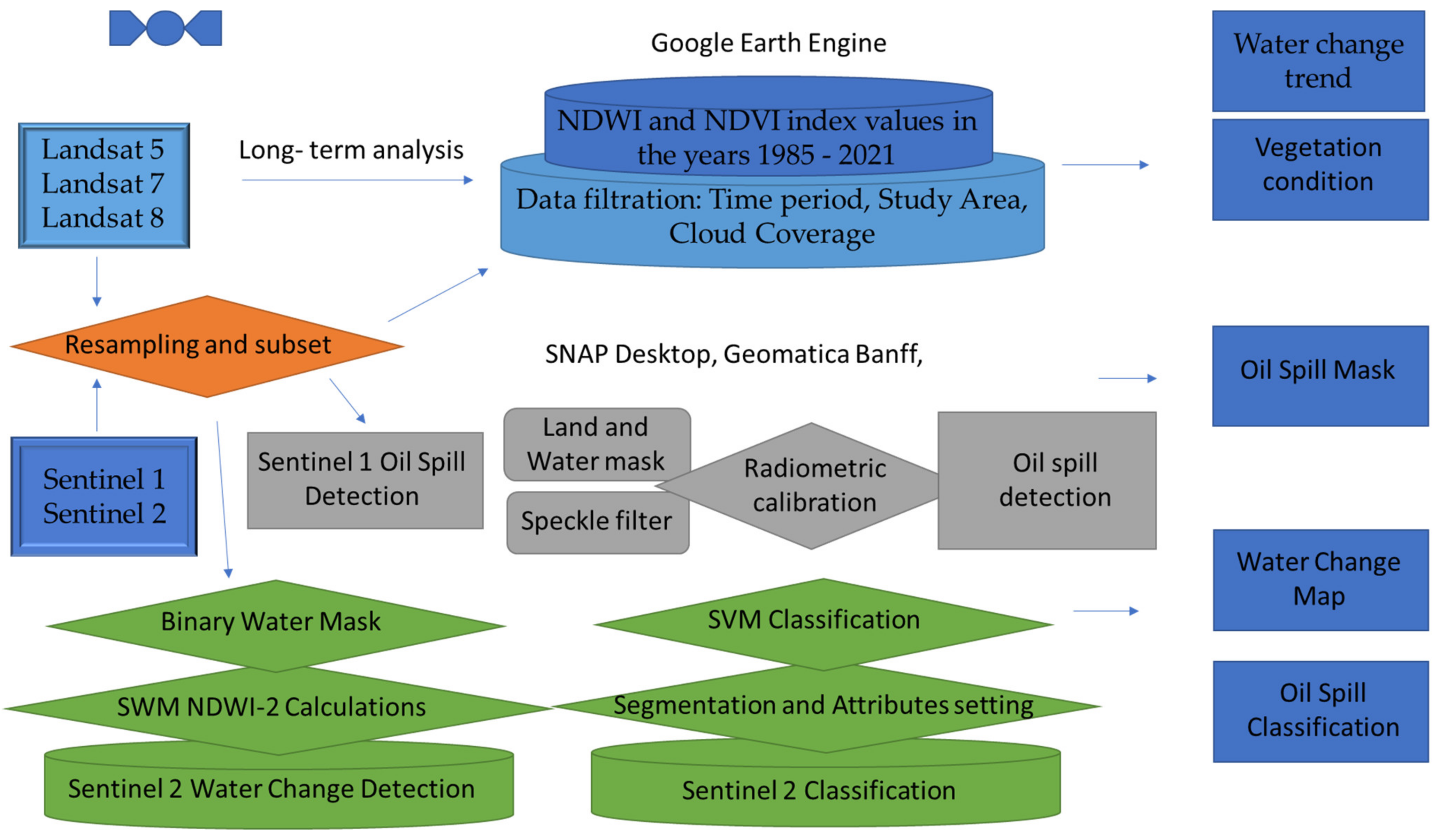
2.2. Methodology Description
2.2.1. Satellite Missions
2.2.2. Indices and Classification Methods
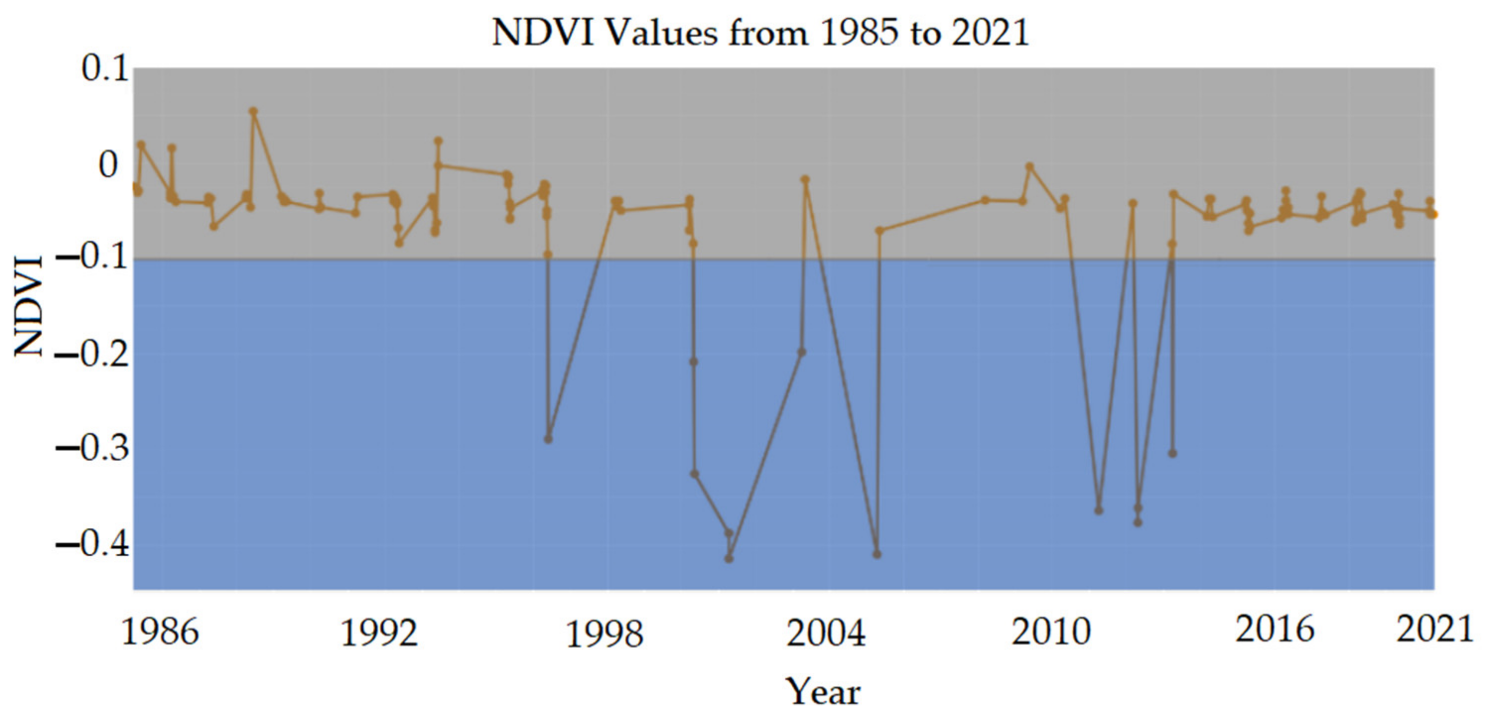
- NDVI
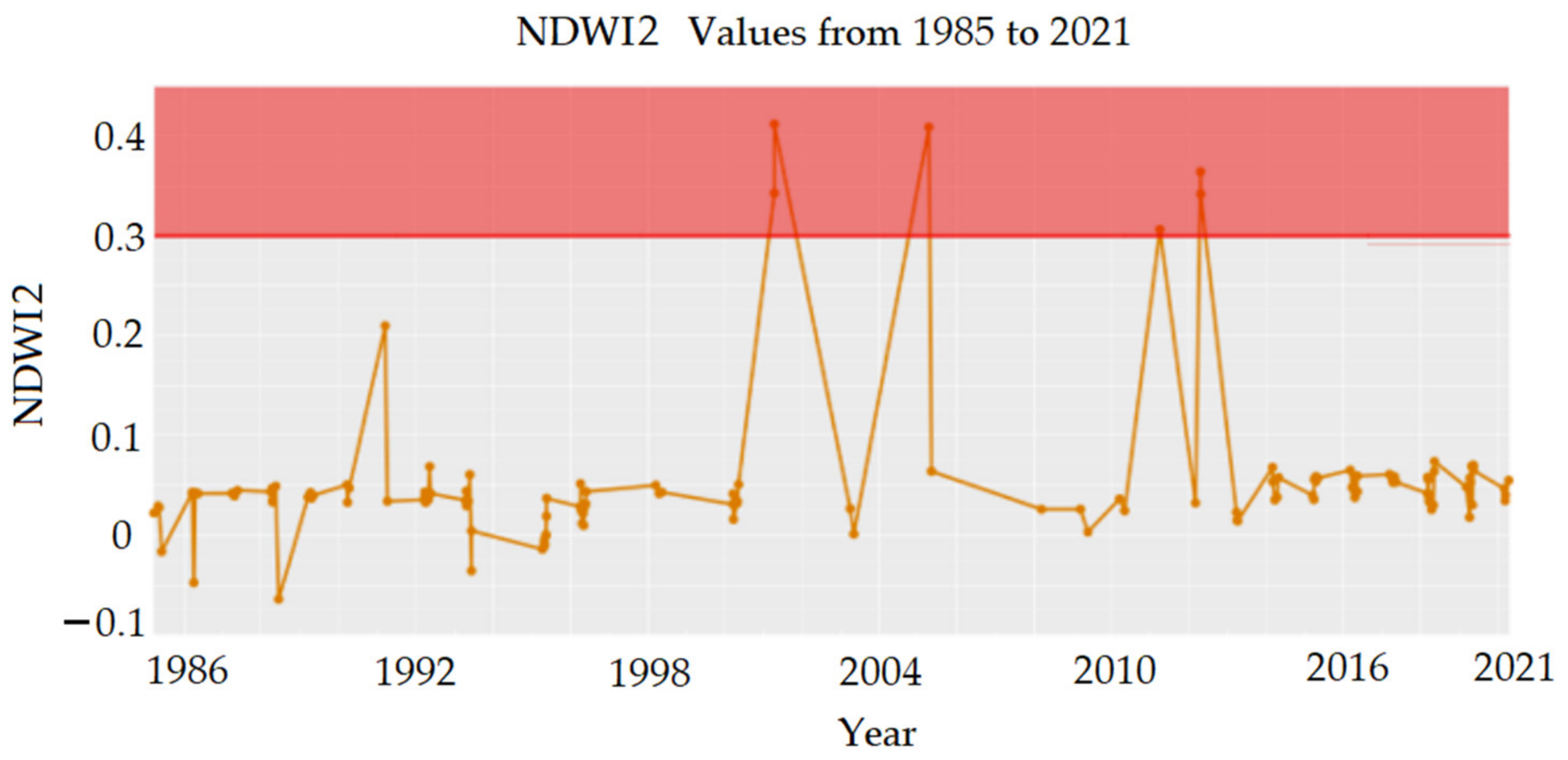
- NDWI2
- NDSII
- SWM
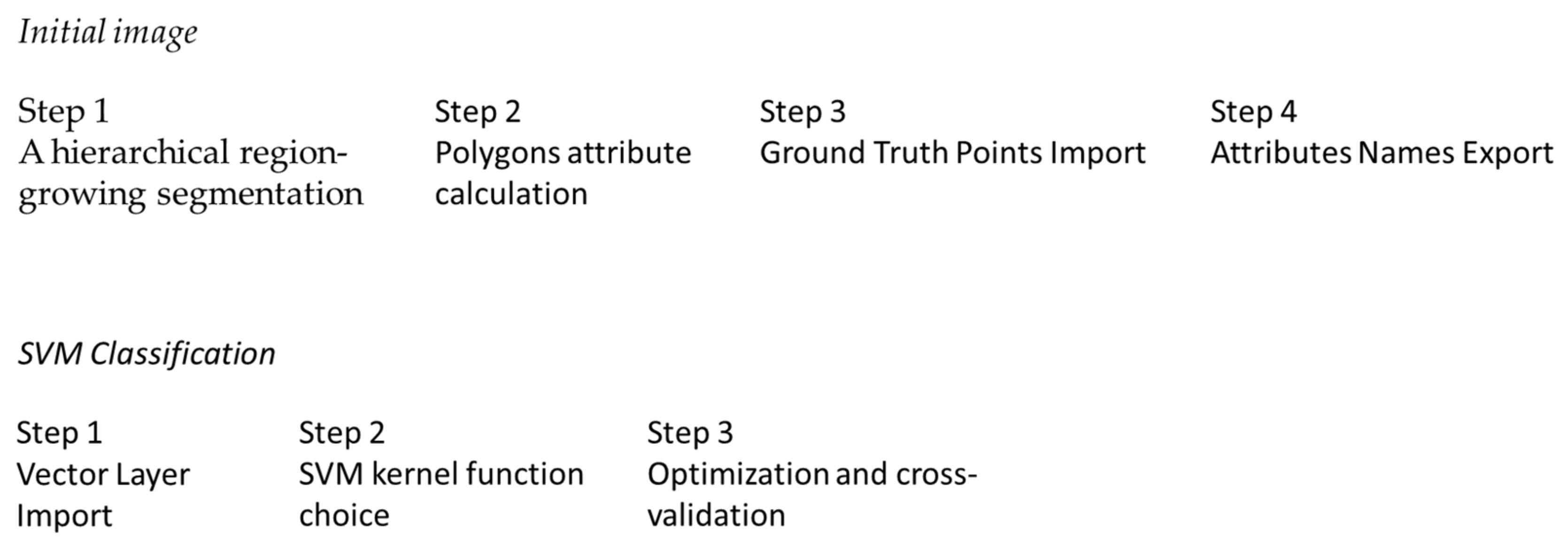
2.2.3. Classification
2.2.4. Short and Long-Term Analysis
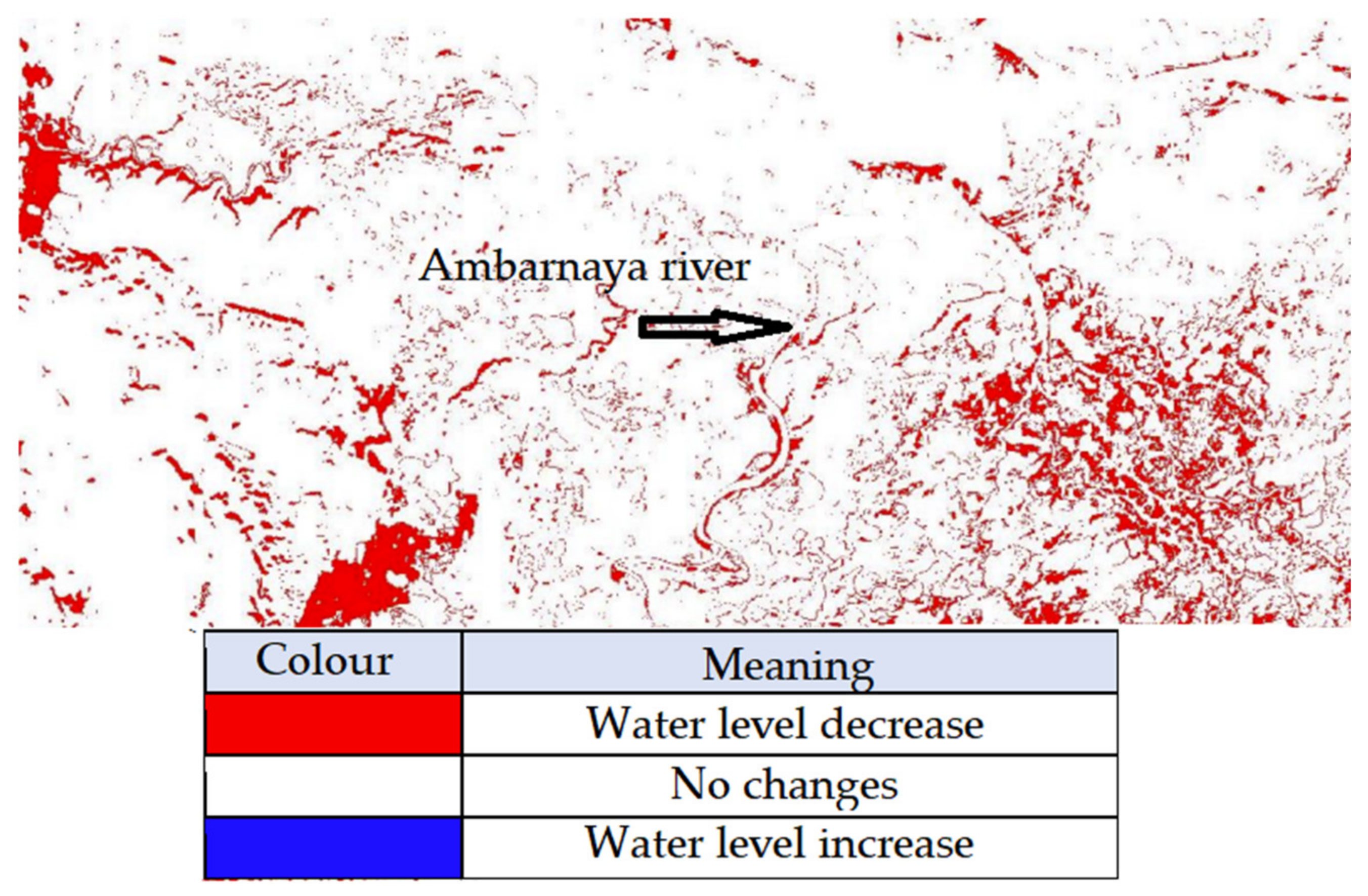
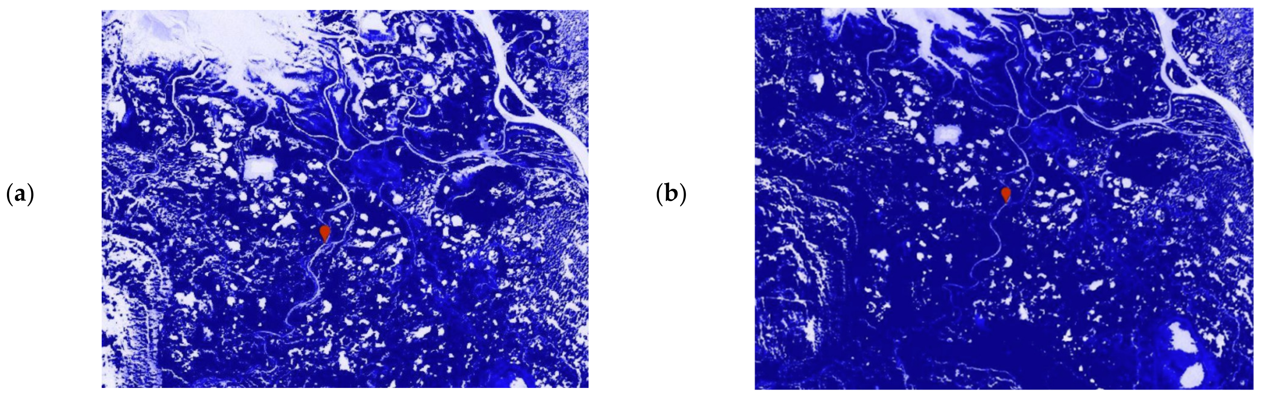
3. Results
4. Discussion
5. Conclusions
Supplementary Materials
Author Contributions
Funding
Institutional Review Board Statement
Informed Consent Statement
Data Availability Statement
Acknowledgments
Conflicts of Interest
Abbreviations
| ETM+ | the Enhanced Thematic Mapper Plus |
| GNSS | Global Navigation Satellite System |
| JRC | Joint Research Centre |
| MSS | Multispectral Scanner System |
| NDSII | Normalized Difference Snow and Ice Index |
| NDVI | Normalized Difference Vegetation Index |
| NDWI2 | Second Normalized Difference Water Index |
| OLI | Operational Land Imager |
| Rosprirodnadzor | The Federal Russian Natural Resourse Surveillance |
| SAR | Syntetic Aperture Radar |
| SNAP | Sentinel Application Platform |
| SVM | Support Vector Machine |
| SWM | Sentinel Water Mask |
| TIRS | Thermal InfraRed Sensor |
| TM | Thematic Mapping |
References
- Startsev, N.; Bhatti, J.S.; Jassal, R.S. Surface CO2 Exchange Dynamics across a Climatic Gradient in McKenzie Valley: Effect of Landforms, Climate and Permafrost. Forests 2016, 7, 279. [Google Scholar] [CrossRef] [Green Version]
- Nyland, K.; Gunn, G.; Shiklomanov, N.; Engstrom, R.; Streletskiy, D. Land Cover Change in the Lower Yenisei River Using Dense Stacking of Landsat Imagery in Google Earth Engine. Remote Sens. 2018, 10, 1226. [Google Scholar] [CrossRef] [Green Version]
- Bennett, M. >Norilsk Oil Spill: “There Are Rivers of Fuel”. Cryopolitics, 22 June 2020. Available online: https://www.cryopolitics.com/2020/06/22/norilsk-oil-spill/(accessed on 17 February 2022).
- Miles, H. The Island of Lost Maps: A True Story of Cartographic Crime; Random House: New York, NY, USA, 2010; ISBN 978-0-375-50151-7. [Google Scholar]
- Hall, S. Mapping the Next Millennium: The Discovery of New Geographies, 1st ed.; Random House: New York, NY, USA, 1992; ISBN 978-0394576350. [Google Scholar]
- Chengchao, W.; Lanxin, M.; Liu, L.H. Spectral radiative properties of seawater-in-oil emulsions in visible-infrared region. J. Quant. Spectrosc. Radiat. Transf. 2021, 272, 107823. [Google Scholar] [CrossRef]
- Kolokoussis, P.; Karathanassi, V. Oil Spill Detection and Mapping Using Sentinel 2 Imagery. J. Mar. Sci. Eng. 2018, 6, 4. [Google Scholar] [CrossRef] [Green Version]
- Nazirova, K.; Lavrova, O. Monitoring of Marine Pollution in the Gulf of Lion Based on Remote Sensing Data. In Proceedings of the 2018 OCEANS—MTS/IEEE Kobe Techno-Oceans (OTO), Kobe, Japan, 28–31 May 2018; pp. 1–5. [Google Scholar] [CrossRef]
- Yang, J.; Wan, J.; Ma, Y.; Zhang, J.; Hu, Y. Characterization analysis and identification of common marine oil spill types using hyperspectral remote sensing. Int. J. Remote Sens. 2020, 41, 7163–7185. [Google Scholar] [CrossRef]
- Dixit, A.; Goswami, A.; Jain, S. Development and Evaluation of a New “Snow Water Index (SWI)” for Accurate Snow Cover Delineation. Remote Sens. 2019, 11, 2774. [Google Scholar] [CrossRef] [Green Version]
- Bonnington, A.; Amani, M.; Ebrahimy, H. Oil Spill Detection Using Satellite Imagery. Adv. Environ. Eng. Res. 2021, 2, 1. [Google Scholar] [CrossRef]
- Fingas, M.; Brown, C.E. A Review of Oil Spill Remote Sensing. Sensors 2018, 18, 91. [Google Scholar] [CrossRef] [Green Version]
- Kurata, N.; Vella, K.; Hamilton, B.; Shivji, M.; Soloviev, A.; Matt, S.; Tartar, A.; Perrie, W. Surfactant-associated bacteria in the near-surface layer of the ocean. Sci. Rep. 2016, 6, 19123. [Google Scholar] [CrossRef] [Green Version]
- Bhangale, U.; Durbha, S.; King, R.; Younan, N.H.; Vatsavai, R. High performance GPU computing based approaches for oil spill detection from multi-temporal remote sensing data. Remote Sens. Environ. 2017, 202, 28–44. [Google Scholar] [CrossRef]
- Pisano, A.; Bignami, F.; Santoleri, R. Oil Spill Detection in Glint-Contaminated Near-Infrared MODIS Imagery. Remote Sens. 2015, 7, 1112–1134. [Google Scholar] [CrossRef] [Green Version]
- Rajendran, S.; Sadooni, F.N.; Al-Kuwari, H.A.-S.; Oleg, A.; Govil, H.; Nasir, S.; Vethamony, P. Monitoring oil spill in Norilsk, Russia using satellite data. Sci. Rep. 2021, 11, 3817. [Google Scholar] [CrossRef] [PubMed]
- Fingas, M. The Challenges of Remotely Measuring Oil Slick Thickness. Remote Sens. 2018, 10, 319. [Google Scholar] [CrossRef] [Green Version]
- Hu, S.C.; Garcia-Pineda, O.; Kourafalou, V.; Le Hénaff, M.; Androulidakis, Y. Remote sensing assessment of oil spills near a damaged platform in the Gulf of Mexico. Mar. Pollut. Bull. 2018, 136, 141–151. [Google Scholar] [CrossRef]
- Sun, S.; Lu, Y.; Liu, Y.; Wang, M.; Hu, C. Tracking an Oil Tanker Collision and Spilled Oils in the East China Sea Using Multisensor Day and Night Satellite Imagery. Geophys. Res. Lett. 2018, 45, 3212–3220. [Google Scholar] [CrossRef]
- Biermann, L.; Clewley, D.; Martinez-Vicente, V.; Topouzelis, K. Finding Plastic Patches in Coastal Waters using Optical Satellite Data. Sci. Rep. 2020, 10, 5364. [Google Scholar] [CrossRef] [Green Version]
- Wettle, M.J.; Daniel, P.A.; Logan, G.; Thankappan, M. Assessing the effect of hydrocarbon oil type and thickness on a remote sensing signal: A sensitivity study based on the optical properties of two different oil types and the HYMAP and Quickbird sensors. Remote Sens. Environ. 2009, 113, 2000–2010. [Google Scholar] [CrossRef]
- Fingas, M.; Brown, C. Review of oil spill remote sensing. Mar. Pollut. Bull. 2014, 83, 9–23. [Google Scholar] [CrossRef] [Green Version]
- Sulfur Dioxide from Norilsk, Russia; Earth Observatory NASA. Available online: https://earthobservatory.nasa.gov/images/36063/sulfur-dioxide-from-norilsk-russia (accessed on 17 February 2022).
- Lu, Y.; Tian, Q.; Wang, J.; Wang, X.; Qi, X. Experimental study on spectral responses of offshore oil slick. Chin. Sci. Bull. 2008, 53, 3937–3941. [Google Scholar] [CrossRef] [Green Version]
- Klemas, V. Tracking Oil Slicks and Predicting their Trajectories Using Remote Sensors and Models: Case Studies of the Sea Princess and Deepwater Horizon Oil Spills. J. Coast. Res. 2010, 265, 789–797. [Google Scholar] [CrossRef] [Green Version]
- Sun, Z.; Zhao, Y.; Yan, G.; Li, S. Study on the hyperspectral polarized reflection characteristics of oil slicks on sea surfaces. Chin. Sci. Bull. 2011, 56, 1596–1602. [Google Scholar] [CrossRef] [Green Version]
- Kolokoussis, P.; Karathanassi, V. Detection of Oil Spills and Underwater Natural Oil Outflow Using Multispectral Satellite Imagery. Int. J. Remote Sens. Appl. 2013, 3, 145–154. [Google Scholar]
- Rajendran, S.; Vethamony, P.N.; Sadooni, F.; Al-Saad Al-Kuwari, H.A.; Al-Khayat, J.; Govil, H.; Nasir, S. Sentinel-2 image transformation methods for mapping oil spill—A case study with Wakashio oil spill in the Indian Ocean, off Mauritius. MethodsX 2021, 8, 101327. [Google Scholar] [CrossRef] [PubMed]
- Gravesen, H.; Ammendrup, H.; Lollike, J. A Railway on Permafrostin Siberia; OMAE (ASME) IV; Arctic/Polar Technology; American Society of Mechanical Engineers: New York, NY, USA, 1995. [Google Scholar]
- Spiridonov, V.V.; Semenov, L.P.; Krivoshein, B.L. Pipeline construction in permafrost regions. In Proceedings of the 2nd International Conference on Permafrost, Yakutsk, USSR, 13–18 July 1973; Sanger, F.J., Hyde, P.J., Eds.; National Academy of Sciences: Washington, DC, USA, 1978. [Google Scholar]
- Sereda, E.; Belyatsky, B.; Krivolutskaya, N. Geochemistry and Geochronology of Southern Norilsk Intrusions, SW Siberian Traps. Minerals 2020, 10, 165. [Google Scholar] [CrossRef] [Green Version]
- Bauduin, S.; Clarisse, L.; Clerbaux, C.; Hurtmans, D.; Coheur, P.-F. IASI observations of sulfur dioxide (SO2) in the boundary layer of Norilsk. J. Geophys. Res. Atmos. 2014, 119, 4253–4263. [Google Scholar] [CrossRef] [Green Version]
- Blais, J.M.; Duff, K.E.; Laing, T.E.; Smol, J.P. Regional Contamination in Lakes from the Noril’sk Region in Siberia, Russia. Water Air Soil Pollut. 1999, 110, 389–404. [Google Scholar] [CrossRef]
- Zubareva, O.N.; Skripal’Shchikova, L.N.; Greshilova, N.V.; Kharuk, V.I. Zoning of Landscapes Exposed to Technogenic Emissions from the Norilsk Mining and Smelting Works. Russ. J. Ecol. 2003, 34, 375–380. [Google Scholar] [CrossRef]
- Environmental Catastrophe Is Declared as One of Biggest Ever Arctic Oil Spills Stretches Out over Taymyr Tundra. Available online: https://thebarentsobserver.com/en/arctic-ecology/2020/06/environmental-catastrophe-declared-one-biggest-ever-arctic-oil-spills (accessed on 17 February 2022).
- Sentinel online: Sentinel-1. Available online: https://sentinel.esa.int/web/sentinel/missions/sentinel-1 (accessed on 17 February 2022).
- Landsat Science. Available online: https://landsat.gsfc.nasa.gov/ (accessed on 17 February 2022).
- Șerban, C.; Maftei, C.; Dobrică, G. Surface Water Change Detection via Water Indices and Predictive Modeling Using Remote Sensing Imagery: A Case Study of Nuntasi-Tuzla Lake, Romania. Water 2022, 14, 556. [Google Scholar] [CrossRef]
- Jiang, W.; Niu, Z.; Wang, L.; Yao, R.; Gui, X.; Xiang, F.; Ji, Y. Impacts of Drought and Climatic Factors on Vegetation Dynamics in the Yellow River Basin and Yangtze River Basin, China. Remote Sens. 2022, 14, 930. [Google Scholar] [CrossRef]
- Meng, Y.; Wei, C.; Guo, Y.; Tang, Z. A Planted Forest Mapping Method Based on Long-Term Change Trend Features Derived from Dense Landsat Time Series in an Ecological Restoration Region. Remote Sens. 2022, 14, 961. [Google Scholar] [CrossRef]
- McFeeters, S.K. Using the Normalized Difference Water Index (NDWI) within a Geographic Information System to Detect Swimming Pools for Mosquito Abatement: A Practical Approach. Remote Sens. 2013, 5, 3544–3561. [Google Scholar] [CrossRef] [Green Version]
- Hall, K.D.; Riggs, G.A.; Salomonson, V.V. Development of methods for mapping global snow cover using moderate resolution imaging spectroradiometer data. Remote Sens. Environ. 1995, 54, 127–140. [Google Scholar] [CrossRef]
- Milczarek, M.; Robak, A.; Gadawska, A. Sentinel Water Mask (SWM)—New index for water detection on Sentinel-2 images, Poster, ESA. In Proceedings of the 7th Advanced Land Training Course on Land Remote Sensing, Gödöllő, Hungary, 4–9 September 2017. [Google Scholar]
- Object-Based SVM Classifier. Available online: https://catalyst.earth/catalyst-system-files/help/references/pciFunction_r/easi/E_oasvmclass.html (accessed on 12 April 2022).
- Janowski, L.; Wroblewski, R.; Rucinska, M.; Kubowicz-Grajewska, A.; Tysiac, P. Automatic classification and mapping of the seabed using airborne LiDAR bathymetry. Eng. Geol. 2022, 301, 106615. [Google Scholar] [CrossRef]
- Ding, S.; Chen, L. Intelligent Optimization Methods for High-Dimensional Data Classification for Support Vector Machines. Intell. Inf. Manag. 2010, 2, 354–364. [Google Scholar] [CrossRef] [Green Version]
- Shirmard, H.; Farahbakhsh, E.; Heidari, E.; Beiranvand Pour, A.; Pradhan, B.; Müller, D.; Chandra, R. A Comparative Study of Convolutional Neural Networks and Conventional Machine Learning Models for Lithological Mapping Using Remote Sensing Data. Remote Sens. 2022, 14, 819. [Google Scholar] [CrossRef]
- Fan, C.-L. Evaluation of Classification for Project Features with Machine Learning Algorithms. Symmetry 2022, 14, 372. [Google Scholar] [CrossRef]
- Hjort, J.; Karjalainen, O.; Aalto, J.; Westermann, S.; Romanovsky, V.E.; Nelson, F.E.; Etzelmüller, B.; Luoto, M. Degrading permafrost puts Arctic infrastructure at risk by mid-century. Nat. Commun. 2018, 9, 5147. [Google Scholar] [CrossRef]
- JRC Yearly Water Classification History, v1.3. Available online: https://developers.google.com/earth-engine/datasets/catalog/JRC_GSW1_3_YearlyHistory (accessed on 23 March 2022).
- Chander, G.L.; Markham, B.; Helder, D.L. Summary of current radiometric calibration coefficients for Landsat MSS, TM, ETM+, and EO-1 ALI sensors. Remote Sens. Environ. 2009, 113, 893–903. [Google Scholar] [CrossRef]
- Liu, Y.; Macfadyen, A.; Zhen-Gang, J.; Weisberg, R. Monitoring and Modeling the Deepwater Horizon Oil Spill: A Record-Breaking Enterprise; John Wiley & Sons: Hoboken, NJ, USA, 2011; Volume 195. [Google Scholar] [CrossRef]
- Presidential Decree of the Russian Federation of May 6, 2018 No.198. About Bases of state Policy of the Russian Federation in the Field of Industrial Safety for the Period Till 2025 and Further Perspective. Available online: https://cis-legislation.com/document.fwx?rgn=106262 (accessed on 12 April 2022).
- Clean-Up Progress Update on the Accident. Available online: https://www.nornickel.com/news-and-media/press-releases-and-news/updates-on-the-clean-up-operation-following-diesel-spill-in-norilsk/ (accessed on 17 February 2022).
- Siberian Heatwave of 2020 almost Impossible without Climate Change. Available online: https://www.worldweatherattribution.org/siberian-heatwave-of-2020-almost-impossible-without-climate-change/ (accessed on 17 February 2022).
- Mallouppas, G.; Ioannou, C.; Yfantis, E.A. A Review of the Latest Trends in the Use of Green Ammonia as an Energy Carrier in Maritime Industry. Energies 2022, 15, 1453. [Google Scholar] [CrossRef]
- Cao, X.; Zhao, T.; Xing, Z. How Do Government Policies Promote Green Housing Diffusion in China? A Complex Network Game Context. Int. J. Environ. Res. Public Health 2022, 19, 2238. [Google Scholar] [CrossRef]
- Nazarko, Ł.; Žemaitis, E.; Wróblewski, Ł.K.; Šuhajda, K.; Zajączkowska, M. The Impact of Energy Development of the European Union Euro Area Countries on CO2 Emissions Level. Energies 2022, 15, 1425. [Google Scholar] [CrossRef]


| CLASS | Training | Test | Total |
|---|---|---|---|
| Water | 88 | 46 | 134 |
| Oil | 28 | 11 | 39 |
| Ground | 81 | 54 | 135 |
| Vegetation | 34 | 19 | 53 |
| Snow | 38 | 19 | 57 |
| Buildings | 18 | 9 | 27 |
| Class Name | Water | Vegetation | Ground | Snow/Ice | Oil | Buildings | Total |
|---|---|---|---|---|---|---|---|
| Water | 46 | 0 | 0 | 0 | 0 | 0 | 46 |
| Vegetation | 0 | 8 | 1 | 0 | 0 | 1 | 10 |
| Ground | 0 | 10 | 51 | 2 | 0 | 2 | 65 |
| Snow/Ice | 0 | 0 | 0 | 17 | 0 | 0 | 17 |
| Oil | 0 | 1 | 1 | 0 | 11 | 0 | 13 |
| Buildings | 0 | 0 | 1 | 0 | 0 | 6 | 7 |
| Total: | 46 | 19 | 54 | 19 | 11 | 9 | |
| Overall accuracy: 87.975% | |||||||
| Overall kappa statistics: 0.839 | |||||||
| 95% Confidence Interval (82.587–93.363%) | |||||||
| Class Name | Producer’s Accuracy | 95% Confidence Interval | User’s Accuracy | 95% Confidence Interval | Kappa Statistics | ||
| Water | 100.000% | (98.913–100.000%) | 100.000% | (98.913–100.000%) | 1.0000 | ||
| Vegetation | 42.105% | (17.273–66.938%) | 80.000% | (50.208–100.000%) | 0.7727 | ||
| Ground | 94.444% | (87.409–100.000%) | 78.462% | (67.698–89.225%) | 0.6728 | ||
| Snow/Ice | 89.474% | (73.043–100.000%) | 100.000% | (97.059–100.000%) | 1.0000 | ||
| Oil | 100.000% | (95.455–100.000%) | 84.615% | (61.156–100.000%) | 0.8346 | ||
| Buildings | 66.667% | (30.313–100.000%) | 85.714% | (52.648–100.000%) | 0.8485 | ||
| Quantity Disagreement: 8.228% | Allocation Disagreement: 3.797% | ||||||
Publisher’s Note: MDPI stays neutral with regard to jurisdictional claims in published maps and institutional affiliations. |
© 2022 by the authors. Licensee MDPI, Basel, Switzerland. This article is an open access article distributed under the terms and conditions of the Creative Commons Attribution (CC BY) license (https://creativecommons.org/licenses/by/4.0/).
Share and Cite
Tysiąc, P.; Strelets, T.; Tuszyńska, W. The Application of Satellite Image Analysis in Oil Spill Detection. Appl. Sci. 2022, 12, 4016. https://doi.org/10.3390/app12084016
Tysiąc P, Strelets T, Tuszyńska W. The Application of Satellite Image Analysis in Oil Spill Detection. Applied Sciences. 2022; 12(8):4016. https://doi.org/10.3390/app12084016
Chicago/Turabian StyleTysiąc, Paweł, Tatiana Strelets, and Weronika Tuszyńska. 2022. "The Application of Satellite Image Analysis in Oil Spill Detection" Applied Sciences 12, no. 8: 4016. https://doi.org/10.3390/app12084016
APA StyleTysiąc, P., Strelets, T., & Tuszyńska, W. (2022). The Application of Satellite Image Analysis in Oil Spill Detection. Applied Sciences, 12(8), 4016. https://doi.org/10.3390/app12084016