
Derivation and Validation of Bandgap Equation Using Serpentine Resonator


Abstract
:1. Introduction
2. Theory
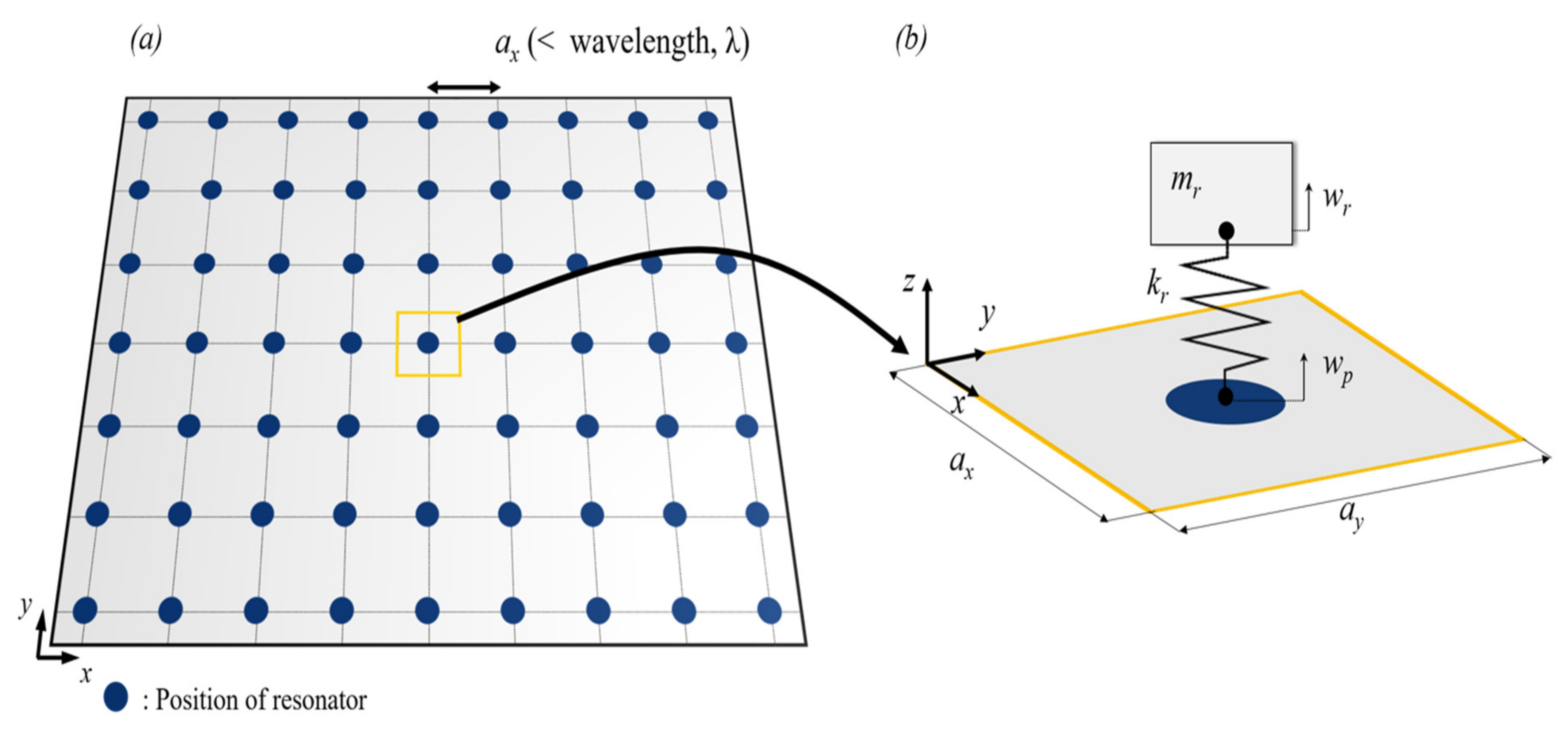
2.1. Bandgap
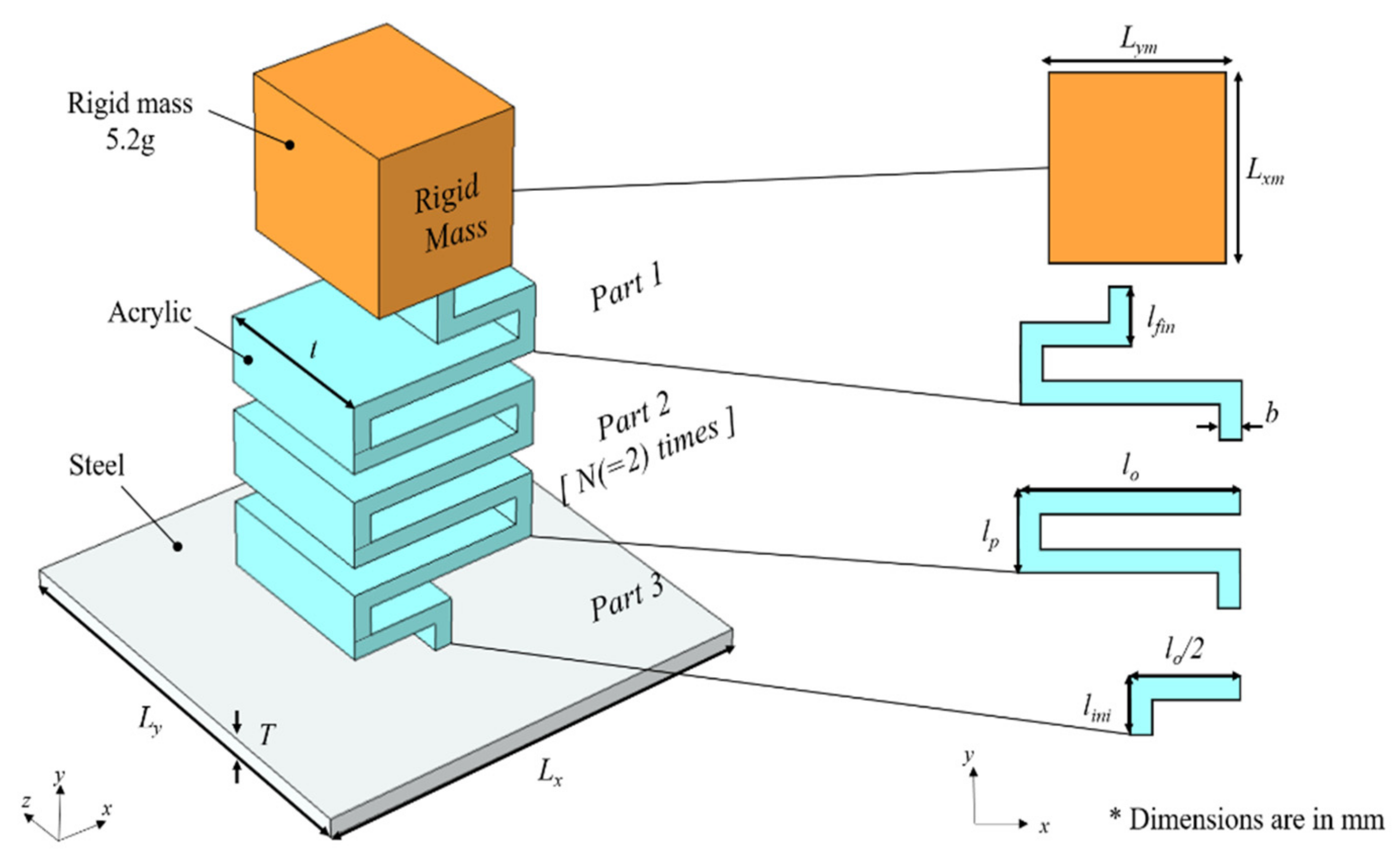
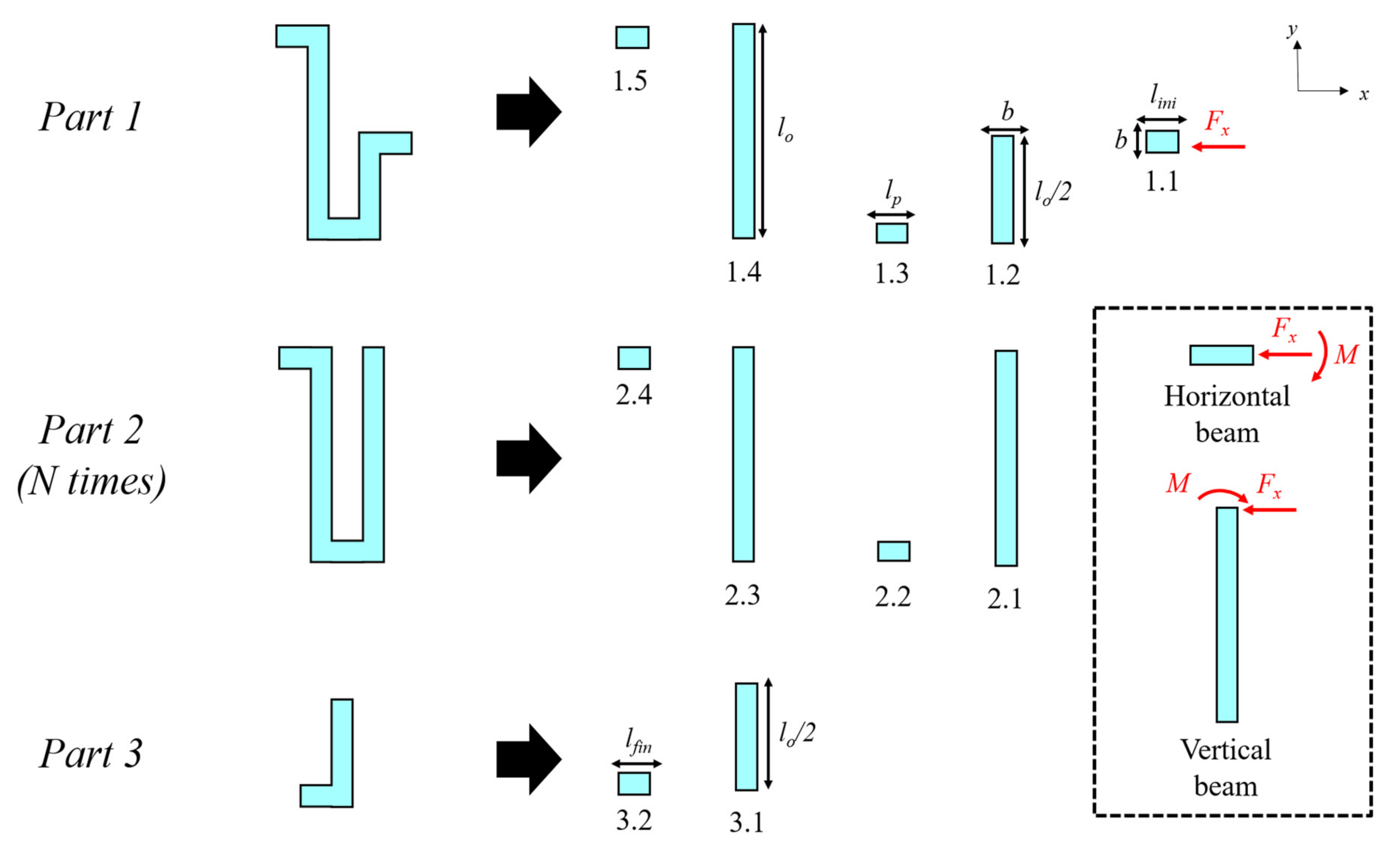
2.2. Serpentine Resonator
3. Numerical Validation
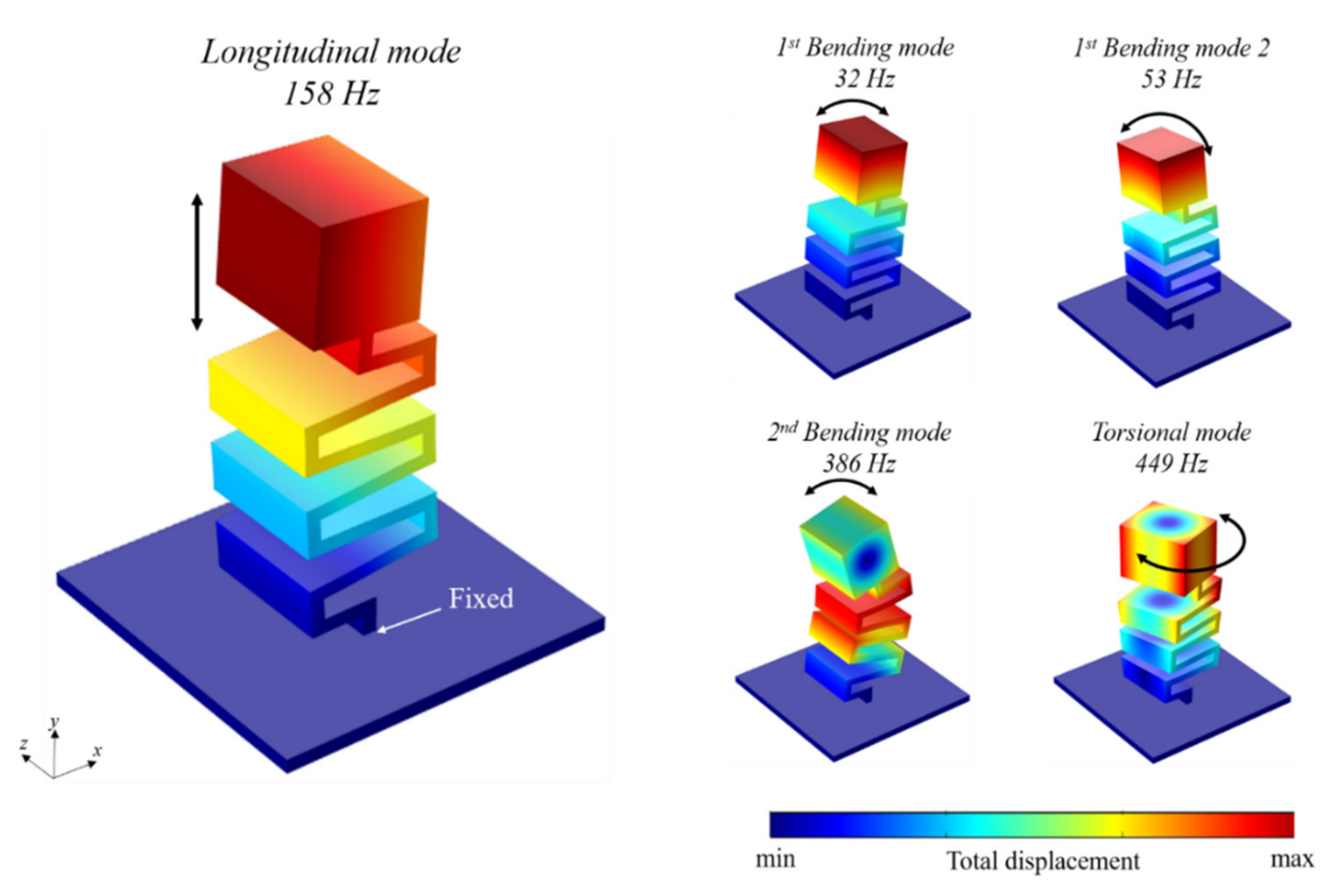
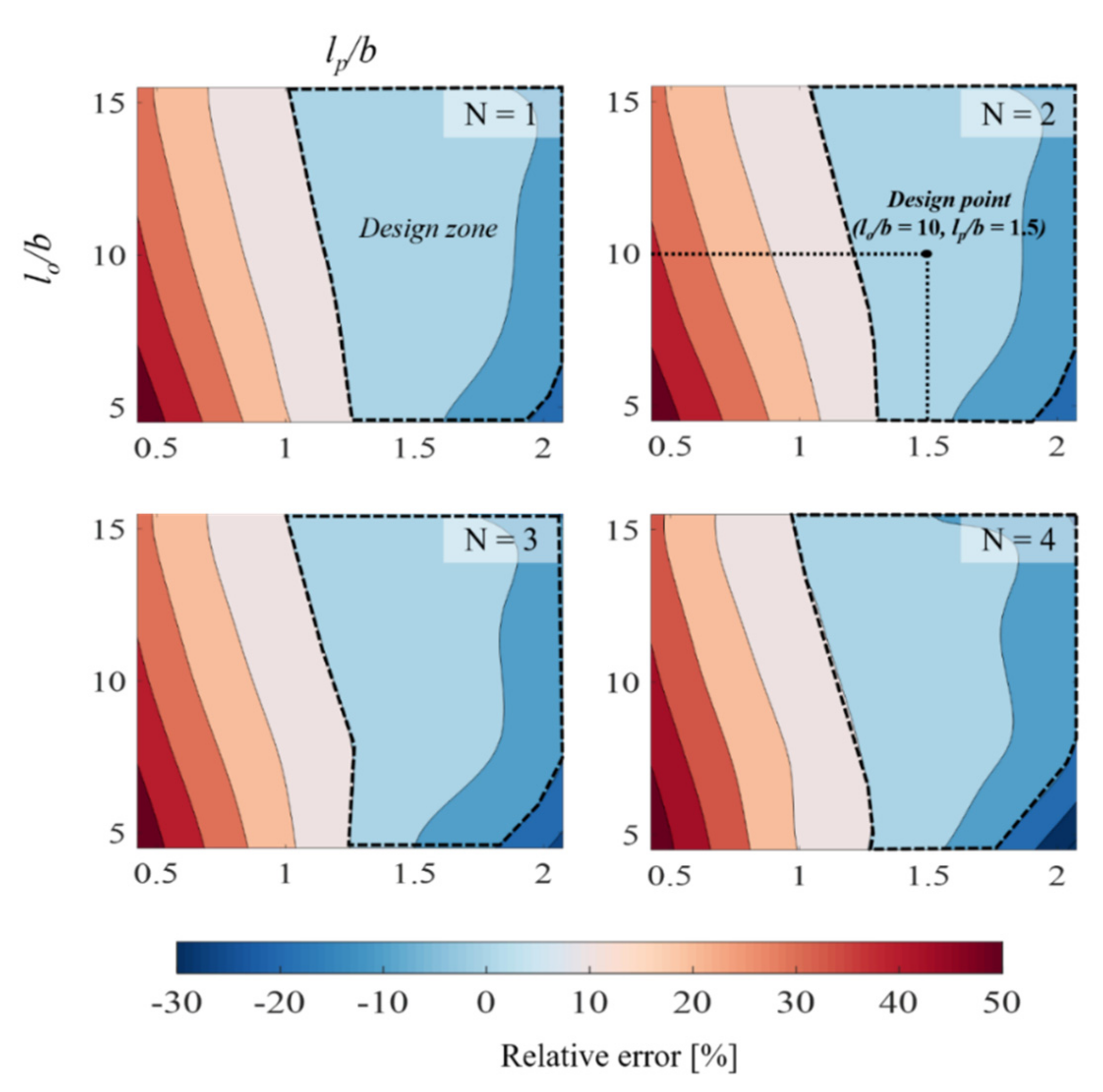
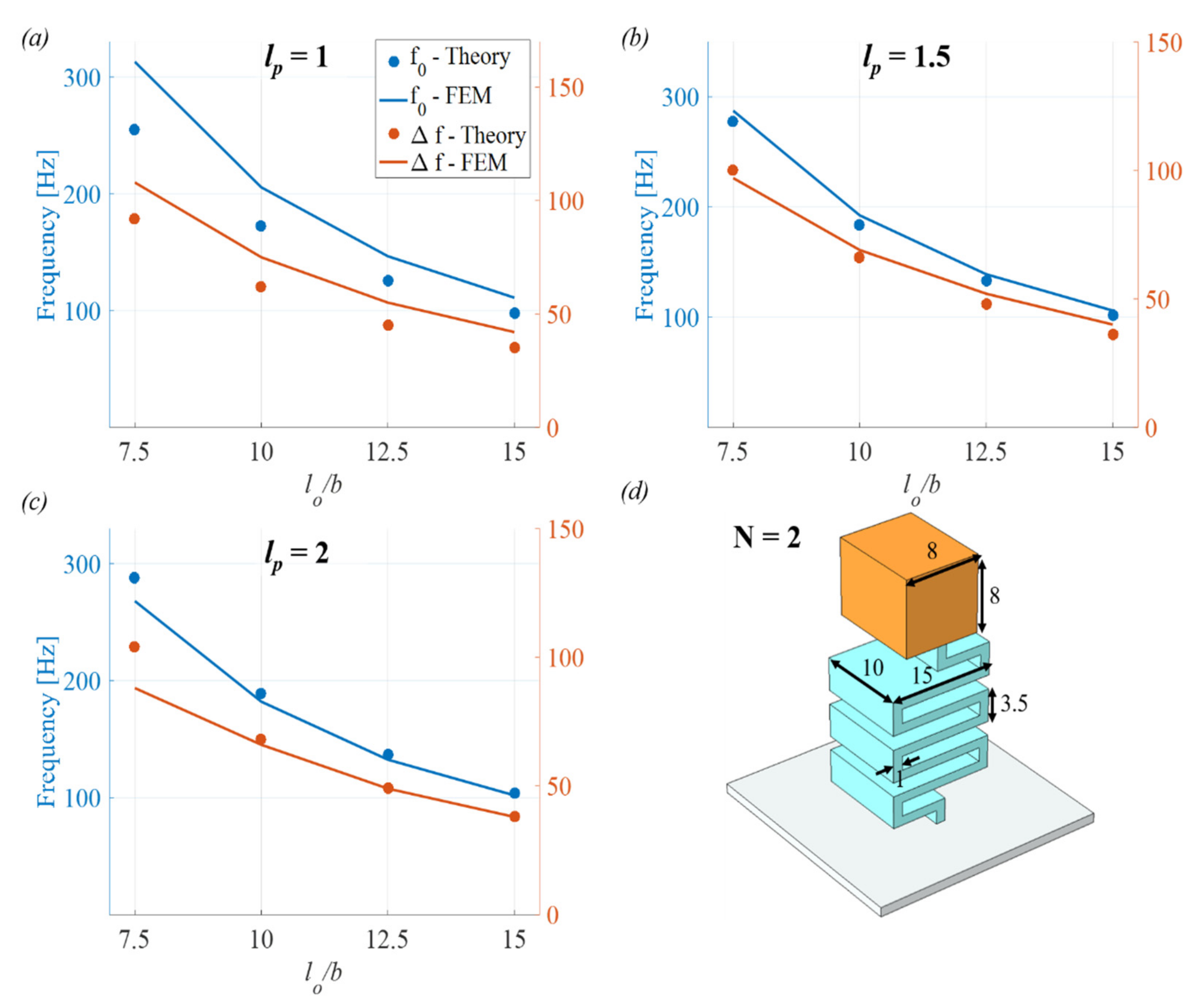
3.1. Resonant Frequency
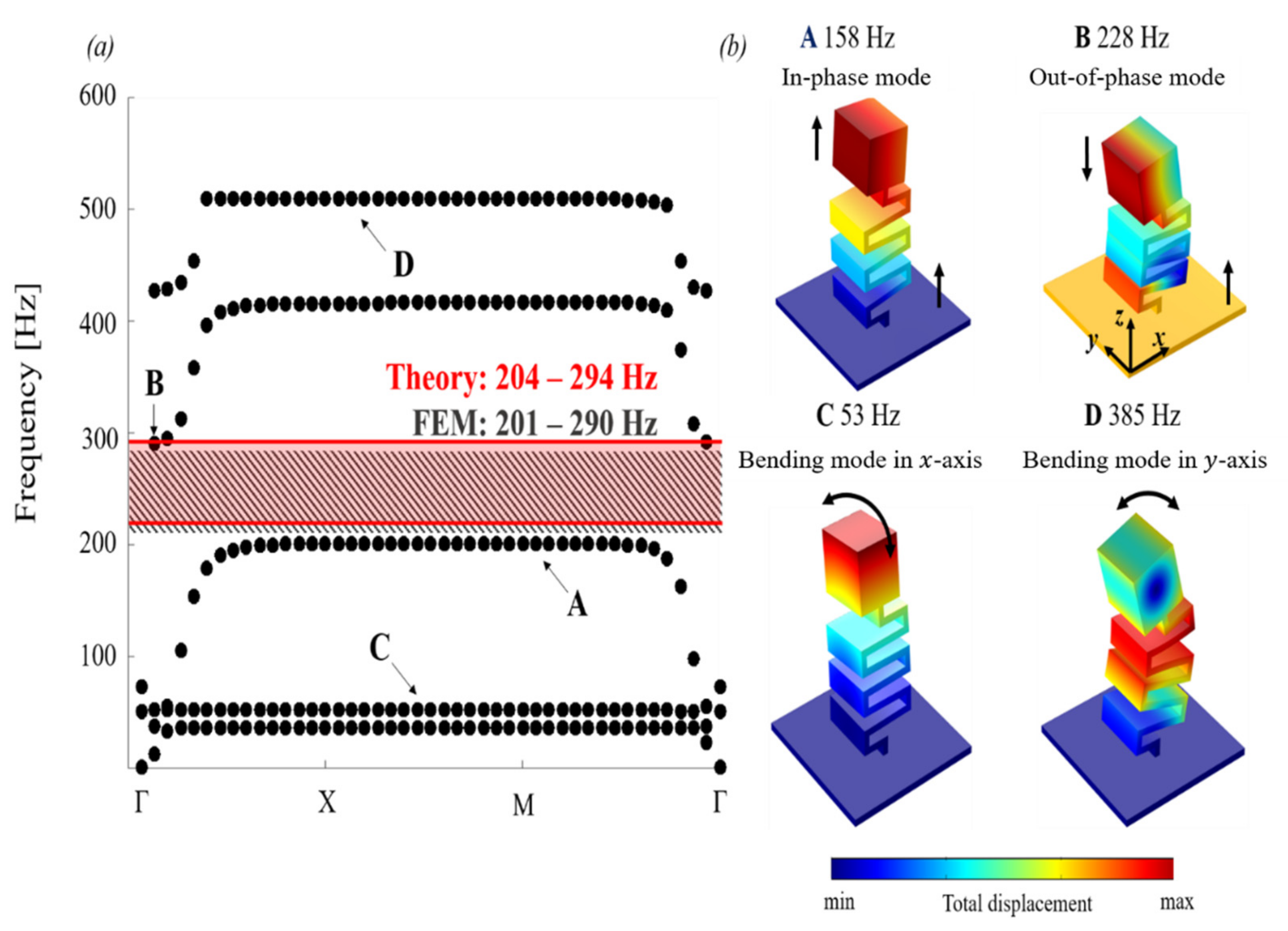
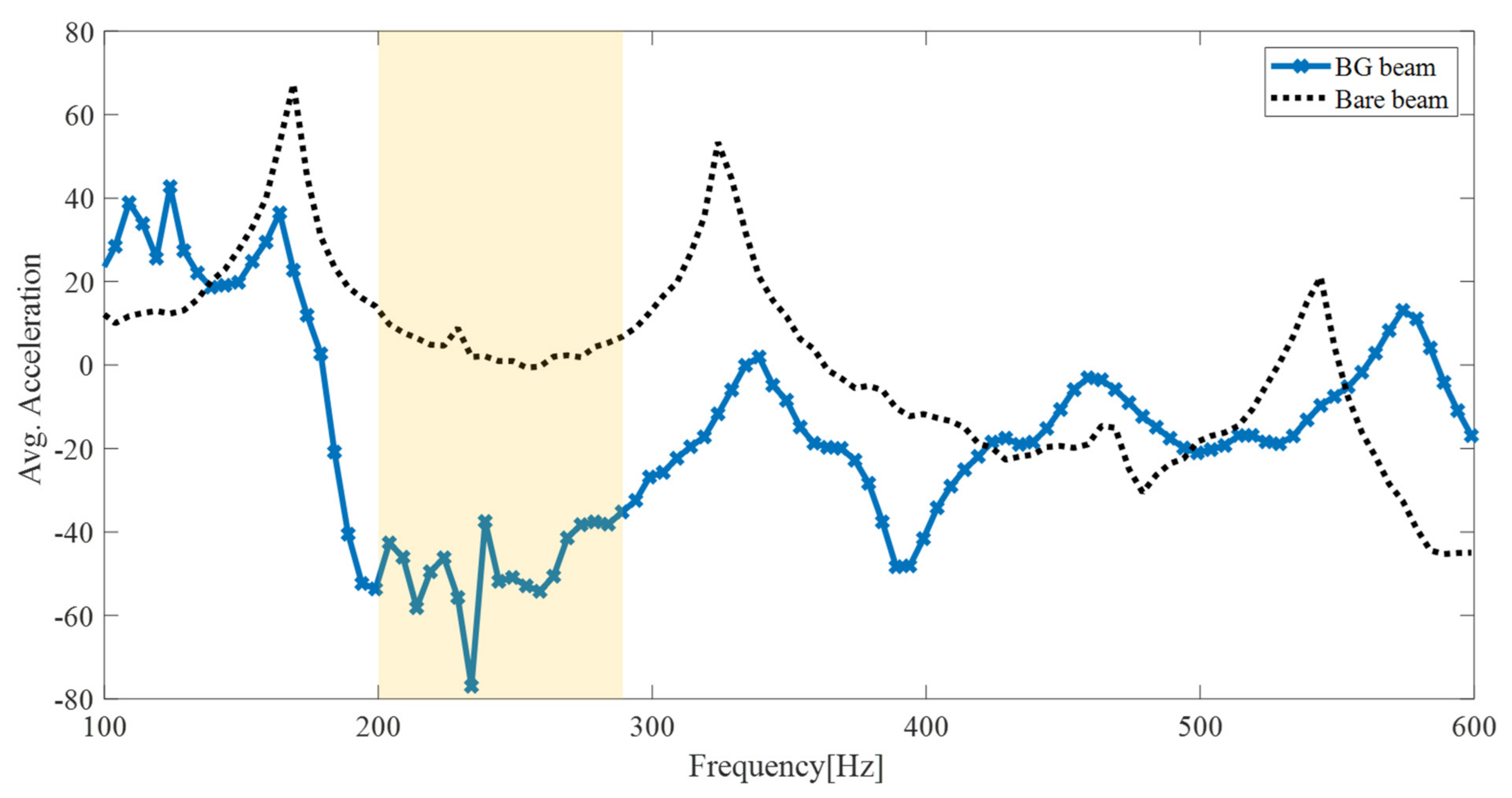
3.2. Bandgap
4. Experimental Validation
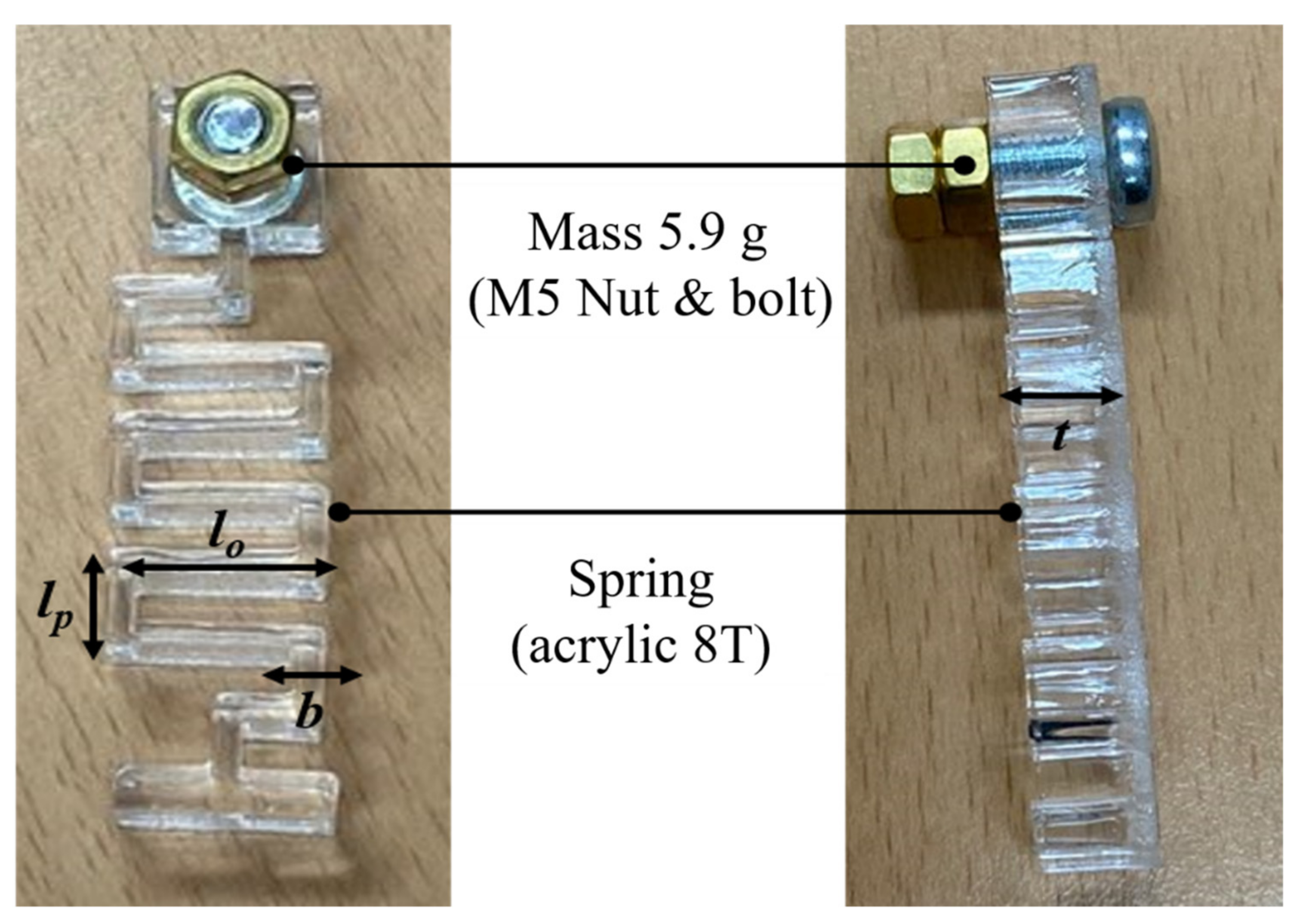
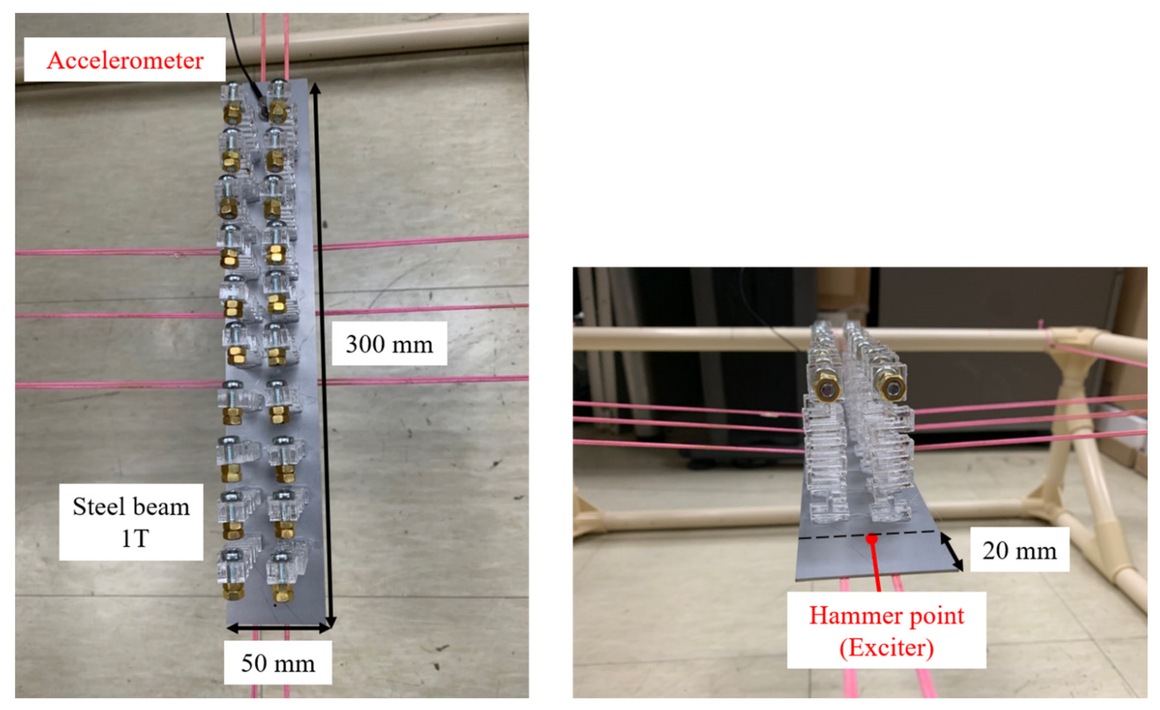
4.1. Fabrication
4.2. Vibration Transmission
5. Conclusions
Author Contributions
Funding
Institutional Review Board Statement
Informed Consent Statement
Data Availability Statement
Conflicts of Interest
References
- Shin, D.; Urzhumov, Y.; Jung, Y.; Kang, G.; Baek, S.; Choi, M.; Park, H.; Kim, K.; Smith, D.R. Broadband electromagnetic cloaking with smart metamaterials. Nat. Commun. 2012, 3, 1213. [Google Scholar] [CrossRef] [PubMed] [Green Version]
- Pendry, J.B. Controlling Electromagnetic Fields. Science 2006, 312, 1780–1782. [Google Scholar] [CrossRef] [Green Version]
- Schurig, D.; Mock, J.J.; Justice, B.J.; Cummer, S.A.; Pendry, J.B.; Starr, A.F.; Smith, D.R. Metamaterial Electromagnetic Cloak at Microwave Frequencies. Science 2006, 314, 977–980. [Google Scholar] [CrossRef] [PubMed] [Green Version]
- Fu, P.; Liu, F.; Ren, G.J.; Su, F.; Li, D.; Yao, J.Q. A broadband metamaterial absorber based on multi-layer graphene in the terahertz region. Opt. Commun. 2018, 417, 62–66. [Google Scholar] [CrossRef]
- Samson, Z.L.; MacDonald, K.F.; De Angelis, F.; Gholipour, B.; Knight, K.; Huang, C.C.; Di Fabrizio, E.; Hewak, D.W.; Zheludev, N. Metamaterial electro-optic switch of nanoscale thickness. Appl. Phys. Lett. 2010, 96, 143105. [Google Scholar] [CrossRef] [Green Version]
- Toal, B.; McMillen, M.; Murphy, A.; Hendren, W.; Atkinson, R.; Pollard, R. Tuneable magneto-optical metamaterials based on photonic resonances in nickel nanorod arrays. Mater. Res. Express 2014, 1, 015801. [Google Scholar] [CrossRef]
- Pai, P.F.; Peng, H.; Jiang, S. Acoustic metamaterial beams based on multi-frequency vibration absorbers. Int. J. Mech. Sci. 2014, 79, 195–205. [Google Scholar] [CrossRef]
- Lee, S.H.; Park, C.M.; Seo, Y.M.; Wang, Z.G.; Kim, C.K. Acoustic metamaterial with negative density. Phys. Lett. A 2009, 373, 4464–4469. [Google Scholar] [CrossRef]
- Ma, G.; Sheng, P. Acoustic metamaterials: From local resonances to broad horizons. Sci. Adv. 2016, 2, e1501595. [Google Scholar] [CrossRef] [Green Version]
- Mei, J.; Ma, G.; Yang, M.; Yang, Z.; Wen, W.; Sheng, P. Dark acoustic metamaterials as super absorbers for low-frequency sound. Nat. Commun. 2012, 3, 756. [Google Scholar] [CrossRef] [Green Version]
- Sui, N.; Yan, X.; Huang, T.Y.; Xu, J.; Yuan, F.G.; Jing, Y. A lightweight yet sound-proof honeycomb acoustic metamaterial. Appl. Phys. Lett. 2015, 106, 171905. [Google Scholar] [CrossRef]
- Liu, Z.; Rumpler, R.; Feng, L. Locally resonant metamaterial curved double wall to improve sound insulation at the ring frequency and mass-spring-mass resonance. Mech. Syst. Signal Process. 2021, 149, 107179. [Google Scholar] [CrossRef]
- Wang, Y.-Z.; Ma, L. Sound insulation performance of membrane-type metamaterials combined with pyramidal truss core sandwich structure. Compos. Struct. 2021, 260, 113257. [Google Scholar] [CrossRef]
- Krushynska, A.O.; Kouznetsova, V.G.; Geers, M.G.D. Towards optimal design of locally resonant acoustic metamaterials. J. Mech. Phys. Solids 2014, 71, 179–196. [Google Scholar] [CrossRef]
- Naify, C.J.; Chang, C.-M.; McKnight, G.; Nutt, S. Transmission loss and dynamic response of membrane-type locally resonant acoustic metamaterials. J. Appl. Phys. 2010, 108, 114905. [Google Scholar] [CrossRef] [Green Version]
- Yu, J.; Nerse, C.; Chang, K.; Wang, S. A framework of flexible locally resonant metamaterials for attachment to curved structures. Int. J. Mech. Sci. 2021, 204, 106533. [Google Scholar] [CrossRef]
- Claeys, C.; Deckers, E.; Pluymers, B.; Desmet, W. A lightweight vibro-acoustic metamaterial demonstrator: Numerical and experimental investigation. Mech. Syst. Signal Process. 2016, 70, 853–880. [Google Scholar] [CrossRef] [Green Version]
- Claeys, C.; de Melo Filho, N.G.R.; Van Belle, L.; Deckers, E.; Desmet, W. Design and validation of metamaterials for multiple structural stop bands in waveguides. Extrem. Mech. Lett. 2017, 12, 7–22. [Google Scholar] [CrossRef] [Green Version]
- De Melo Filho, N.G.R.; Belle, V.L.; Claeys, C.; Deckers, E.; Desmet, W. Dynamic mass based sound transmission loss prediction of vibro-acoustic metamaterial double panels applied to the mass-air-mass resonance. J. Sound Vib. 2019, 442, 28–44. [Google Scholar] [CrossRef]
- Sangiuliano, L.; Claeys, C.; Deckers, E.; Desmet, W. Influence of boundary conditions on the stop band effect in finite locally resonant metamaterial beams. J. Sound Vib. 2020, 473, 115225. [Google Scholar] [CrossRef]
- Nateghi, A.; Belle, V.L.; Claeys, C.; Deckers, E.; Pluymers, B.; Desmet, W. Wave propagation in locally resonant cylindrically curved metamaterial panels. Int. J. Mech. Sci. 2017, 127, 73–90. [Google Scholar] [CrossRef]
- Wang, Q. Bandgap properties in metamaterial sandwich plate with periodically embedded plate-type resonators. Mech. Syst. Signal Process. 2021, 13, 107375. [Google Scholar] [CrossRef]
- Jung, J.; Kim, H.G.; Goo, S.; Chang, K.J.; Wang, S. Realisation of a locally resonant metamaterial on the automobile panel structure to reduce noise radiation. Mech. Syst. Signal Process. 2019, 122, 206–231. [Google Scholar] [CrossRef]
- Chang, I.-L.; Liang, Z.-X.; Kao, H.-W.; Chang, S.-H.; Yang, C.-Y. The wave attenuation mechanism of the periodic local resonant metamaterial. J. Sound Vib. 2018, 412, 349–359. [Google Scholar] [CrossRef]
- Fang, X.; Wen, J.; Yin, J.; Yu, D. Wave propagation in nonlinear metamaterial multi-atomic chains based on homotopy method. AIP Adv. 2016, 6, 121706. [Google Scholar] [CrossRef] [Green Version]
- Sugino, C.; Leadenham, S.; Ruzzene, M.; Erturk, A. On the mechanism of bandgap formation in locally resonant finite elastic metamaterials. J. Appl. Phys. 2016, 120, 134501. [Google Scholar] [CrossRef]
- Barillaro, G.; Molfese, A.; Nannini, A.; Pieri, F. Analysis, simulation and relative performances of two kinds of serpentine springs. J. Micromech. Microeng. 2005, 15, 736–746. [Google Scholar] [CrossRef]
- Chou, H.-M.; Lin, M.-J.; Chen, R. Investigation of mechanics properties of an awl-shaped serpentine microspring for in-plane displacement with low spring constant-to-layout area. J. Micro/Nanolith. MEMS MOEMS 2016, 15, 035003. [Google Scholar] [CrossRef]
- Park, B.; Afsharipour, E.; Chrusch, D.; Shafai, C.; Andersen, D.; Burley, G. Large displacement bi-directional out-of-plane Lorentz actuator array for surface manipulation. J. Micromech. Microeng. 2017, 27, 085005. [Google Scholar] [CrossRef]
- Lishchynska, M.; Cordero, N.; Slattery, O.; O’Mahony, C. Spring Constant Models for Analysis and Design of MEMS Plates on Straight or Meander Tethers. Sens. Lett. 2006, 4, 200–205. [Google Scholar] [CrossRef]


| Symbol | Definition |
|---|---|
| Lx | Length of the plate in x direction |
| Lz | Length of the plate in z direction |
| T | Thickness of the plate |
| Lxm | Length of the rigid mass in x direction |
| Lym | Length of the rigid mass in y direction |
| t | Thickness of the serpentine beams |
| lini | Length of the initial beam |
| lfin | Length of the final beam |
| lo | Length of the beam orthogonal to the y-axis (vertical) |
| lp | Length of the beam parallel to the y-axis (horizontal) |
| b | Width of the serpentine beams |
| lo | lp | b | t | Lxm | Lym | Lxh | Lyh | T |
|---|---|---|---|---|---|---|---|---|
| 8.75 mm | 2 mm | 1 mm | 10 mm | 8 mm | 8 mm | 25 mm | 25 mm | 1 mm |
| lo | lp | b | t | Lxm | Lym | Lxh | Lyh | T |
|---|---|---|---|---|---|---|---|---|
| 15 mm | 3 mm | 2 mm | 8 mm | 12 mm | 12 mm | 25 mm | 25 mm | 1 mm |
| Sample | 1 | 2 | 3 | 4 | 5 | Average |
|---|---|---|---|---|---|---|
| Resonance [Hz] | 189 | 188 | 193 | 190 | 186 | 189 |
Publisher’s Note: MDPI stays neutral with regard to jurisdictional claims in published maps and institutional affiliations. |
© 2022 by the authors. Licensee MDPI, Basel, Switzerland. This article is an open access article distributed under the terms and conditions of the Creative Commons Attribution (CC BY) license (https://creativecommons.org/licenses/by/4.0/).
Share and Cite
Yu, J.; Jung, J.; Wang, S. Derivation and Validation of Bandgap Equation Using Serpentine Resonator. Appl. Sci. 2022, 12, 3934. https://doi.org/10.3390/app12083934
Yu J, Jung J, Wang S. Derivation and Validation of Bandgap Equation Using Serpentine Resonator. Applied Sciences. 2022; 12(8):3934. https://doi.org/10.3390/app12083934
Chicago/Turabian StyleYu, Junmin, Jaesoon Jung, and Semyung Wang. 2022. "Derivation and Validation of Bandgap Equation Using Serpentine Resonator" Applied Sciences 12, no. 8: 3934. https://doi.org/10.3390/app12083934
APA StyleYu, J., Jung, J., & Wang, S. (2022). Derivation and Validation of Bandgap Equation Using Serpentine Resonator. Applied Sciences, 12(8), 3934. https://doi.org/10.3390/app12083934