1. Introduction
Hyperspectral image (HSI) classification is a pixel-by-pixel classification of images based on the spectral and spatial characteristics of target objects. HSIs contain hundreds of narrow and continuous spectral bands and are remote-sensing images that combine two spatial dimensions and one spectral dimension into a data cube. Compared with traditional remote sensing images, the ability of HSIs to analyze ground objects has significantly improved. Some special samples in hyperspectral images have similar colors. Close spectral characteristics and material variability results in minimal inter-class variability in the samples, which will lead to the decline of image classification accuracy and generate a large number of noise points in the classification results. Experts in the field have carried out research from various directions on the negative effects of spectrally similar objects in hyperspectral images. In [
1], VSS Peddinti et al. proposed a method for hyperspectral image simulation of similar spectra using a distance function. This study concentrates on obtaining similar spectra using distance functions. The Chebyshev distance and spectral angle mapper (SAM) distances are combined to get the advantage of both the distance of vector coordinates and the pattern of the spectra. The simulated hyperspectral image is validated with the AVIRIS image using normalized cross-correlation to obtain each pixel’s correlation. The spectral-spatial-based methods aim to extract the spectral and spatial features simultaneously for classification. It can effectively improve the classification accuracy of similar spectral features. In [
2], a lightweight spectral-similarity-based SpaAM was designed by Li N et al. to capture the relevant spatial areas. It describes the spatial distribution of homogeneous pixels and interfering pixels implicitly, which weakens the interfering pixels from the neighborhoods of the center pixel. In this module, the spectral similarities between the center pixel and its neighborhoods are measured by the efficient Euclidean distance. The above studies showed that the distance function is a powerful tool for evaluating the spectral similarity of ground objects.
Hyperspectral data also contains a significant amount of redundant information. To avoid the Hughes Phenomenon [
3,
4], a dimensionality reduction (DR) of HSIs is the first task before classification. Due to the complexity of spectral features, the quality of feature selection will directly affect the classification effect. The research on dimensionality reduction of HSIs has always been an open challenge in the field of hyperspectral applications.
HSI dimensionality reduction can be divided into two categories: feature extraction (FE) and feature selection (FS). FE is to convert high-dimensional data into low-dimensional data through mapping and transformation. The FS of hyperspectral images, that is, band selection, is to select the most effective band subset from all bands, which is essentially a combinatorial optimization problem.
The advantage of feature extraction is that it reduces high-dimensional data to low-dimensional in a rapid and direct manner. Its representative methods are Principal Component Analysis (PCA) [
5,
6] and Linear Discriminant Analysis (LDA) [
7,
8]. Local feature-based manifold learning [
9,
10] and sparse representation [
11] are also important hyperspectral feature extraction methods. At the same time, feature extraction can also combine two different features of space and spectrum for DR [
12]. FE is the goal of reducing dimensionality from a mathematical point of view, but while reducing the dimensionality, it also loses the physical information of ground objects, radiations or reflections contained in the original band. Such results are often not conducive to the classification of hyperspectral remote sensing [
13]. The hyperspectral wavelengths obtained by feature selection do not change mathematically, retain the original features and information of the HSI to the greatest extent, and the number of output wavelengths can be controlled by the corresponding adjustment. Therefore, in order to obtain a specific small number of wavelength combinations with a large amount of information, this paper uses the feature selection method.
A heuristic algorithm is a common means of feature selection [
14,
15,
16,
17]. Among them, Particle Swarm Optimization (PSO) [
18] is one of the most popular algorithms to effectively solve the wavelength combination optimization problem because of its advantages of easy implementation and fast convergence. In [
16], Lishuan Hu et al. proposed an improved DR method of Binary Particle Swarm Optimization with Mutation Mechanism (MNBPSO), and used MNBPSO to simultaneously perform band selection and support vector machine parameter determination. The results showed that the method is more accurate than the results obtained by the SVM and SVM+BPSO algorithms. At the same time, subspace decomposition [
18,
19,
20,
21] is another representative wavelength selection idea. One of its strategies is to use the “blocking” feature of the colormap for the band correlation coefficient matrix to divide all the bands into several subspaces and select high-quality wavelengths from them respectively. In [
21], Lishuan Hu et al. proposed the Improved Optimum Index Factor (IOIF). By selecting the bands with the largest amount of information from different subspaces, IOIF can quickly select the bands with the largest amount of information and the smallest correlation, effectively avoiding the phenomenon of band-centralized selection, reducing the band base participating in the optimal exponential operation and improving the efficiency of the algorithm.
However, the two methods mentioned above are based on a single criterion for wavelength selection because the spectral characteristics between wavelengths of objects with similar colors images are more similar and correlated than ordinary objects images. The DR of a single standard can easily select wavelengths with concentrated bands, large information redundancy, and small differences in spectral characteristics, resulting in a decrease in classification accuracy. In order to satisfy the selected wavelength subsets with less correlation, more information and greater spectral differences are required between ground objects at the same time.
Based on the information calculation model of the local band index (LBI) in the IOIF method and heuristic algorithm for wavelength selection, this paper proposes a new HSI dimensionality reduction method: LBI-BPSO (Binary Particle Swarm Optimization with Local Band Index). Firstly, the amount of information for all wavelengths is calculated by LBI, and the data are sorted and screened according to the amount of information. Further, GA-BPSO (Particle Swarm Optimization with a Genetic Algorithm) is used to optimize the above hyperspectral data subset, and the optimal wavelength combination that meets the requirements is the final result. Finally, LBI-BPSO, IOIF and GA-BPSO are used for wavelength selection, respectively, combined with SVM to classify the simulation data set established in this paper and show their performance evaluation and visual classification results.
The specific objectives of this paper are as follows:
Section 2 briefly introduces the IOIF algorithm for DR of HSI based on the amount of information and the GA-BPSO algorithm with the inter-class distance as the objective function;
Section 3 proposes a novel wavelength selection algorithm that combines information amount and inter-class separability: LBI-BPSO;
Section 4 introduces the sample measurement experiments and the process of establishing hyperspectral simulation images;
Section 5 uses three methods for wavelength selection of simulated HSI, respectively. The DR performance and discussion of LBI are reported in this section, and a comprehensive comparison is made with the effect of IOIF and BPSO. Finally, conclusions and future works are presented in
Section 6.
2. Related Methods
In order to avoid the Hughes Phenomenon caused by redundant information in HSIs, a common method is to process hyperspectral images by means of dimensionality reduction. Band selection for hyperspectral data should consider three factors [
19]:
The information contained in the band or the band combination;
The correlation among the bands;
The spectral response of the ground objects to be identified.
Therefore, the optimal band combination is one with a large amount of information, the small correlation between bands, a large difference in reflectance values of ground objects and good separability between ground objects. The following introduces the IOIF algorithm based on the amount of information as the selection criterion and the GA-BPSO with the inter-class distance as the objective function.
2.1. Improved Optimum Index Factor (IOIF)
A basic principle of wavelength selection for HSI is that the information redundancy between wavelengths in the obtained band subset is small and independent. It can be described by the correlation coefficient matrix, which is calculated by the following Equations (1) and (2) used for the correlation coefficient:
where
n denotes the total number of bands of the HSI and
is the correlation coefficient between the band
i and
j:
where
m is the total number of samples, that is, the total number of pixels in a band image,
is the corresponding vector of the spectral image of the band
,
and
are the mean values of band
i and
j. The smaller the correlation between the selected wavelengths, the higher the independence of the information it contains, and the smaller the information redundancy.
In addition, the selected wavelengths should contain more information. In 1982, Chavez et al. proposed the Optimum Index Factor (OIF) method [
22] to evaluate the optimal band combination by calculating the ratio of the sum of the standard deviations of the bands to the sum of the correlation coefficients. In 2018, Hu Lishuan proposed a new band selection method Improved OIF (IOIF) [
21] based on the OIF information calculation method. In the band subspace, the Local Band Index method (LBI) was used to filter out high-quality band sets. Then, combine the bands from the different sets of high-quality bands and calculate the IOIF value. This method effectively avoids the phenomenon of centralized selection of bands, reduces the number of band bases involved in the operation, and improves the efficiency of the algorithm.
The local band index method is an adaptive band selection method that comprehensively considers the information content and local independence of the image. The LBI is calculated as in the following Equation (3):
where
is the correlation coefficient between band
i−1 and band
i,
is the correlation coefficient between band
i and band
i+1, the average of the two represents the local correlation of band
i, and
is the mean square deviation of band
i.
IOIF is defined as in Equation (4):
where
i,
j and
k are three high-quality bands from different subspaces,
S is the mean square error, and
is the absolute value of the correlation coefficient.
The set of bands selected by IOIF is very similar to the graph of the original bands and contains the richest information of the original bands. After verification by the RBF-SVM classifier, the classification accuracy obtained by the IOIF DR method is higher than the traditional OIF and PCA algorithms. However, this method mainly takes the information of wavelength combination as the basis of wavelength selection.
For the classification of objects with similar colors and close spectrum, a high amount of information is not enough to meet the needs of improving the classification accuracy, and the separability between the selected spectral objects should be further considered.
2.2. Binary Particle Swarm Optimization with Genetic Mechanism (GA-BPSO)
Taking advantage of the heuristic algorithm, aiming at the maximum distance between classes [
23,
24,
25], the wavelength’s combination with the best inter-class separability in the spectral feature space of HSIs can be searched. In this paper, the BPSO with the introduction of a genetic mechanism is selected to obtain the spectral features of ground objects that are easy to be distinguished by the classifier.
The standard PSO algorithm is used to solve the optimization problem in continuous space; however, in terms of discrete space, the discrete binary particle swarm optimization (BPSO) must be used. BPSO [
26] was proposed by Kennedy and Eberhart in 1997 and is widely used in optimization combinatorial problems. This method computationally preserves the classical “position-velocity” update rule. It adopts binary coding and represents the value and change of particle state through 0–1 on each bit. Let the position of the particle
i be
,
; the velocity be
,
; the optimal historical position of the individual is
,
; the overall historical optimal position is
,
. The formula for updating the velocity of particle
i in the
d dimension is as shown in Equation (5):
where
k is the number of iterations,
i and
d represent the particle
i and its dimension, respectively, and
is the inertia weight, which represents the influence of the current speed of the particle on the speed of the next generation.
and
are learning factors, which represent the learning ability of particles to their own experience and group experience, and
and
are random numbers in the interval [0, 1]. In this paper, the convex function decrement method is used to adjust
[
27,
28], and the strategy of decreasing the value of
and increasing the value of
is adopted [
29,
30].
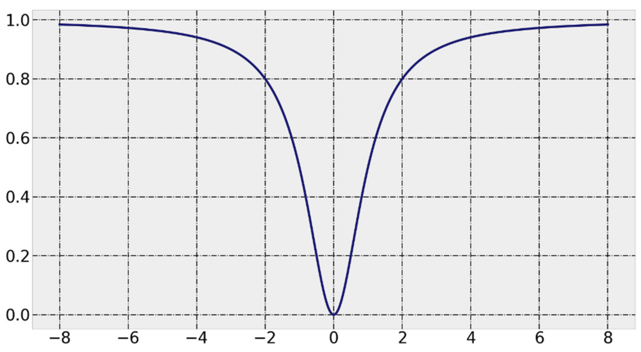
In this paper, a V-shaped [
31] transfer function is used, and the function curve and expression are shown in
Figure 1 and Equation (6), respectively, and Equation (7) is the particle position update formula. In these two equations,
k represents the number of iterations,
i and
d represent the particle
i and its dimension, respectively, and
is a random number in the interval [0, 1].
represents the complement of
, i.e., from 0 to 1 or from 1 to 0.
To further strengthen the BPSO search ability, it is usually advised to introduce the mutation and crossover mechanism in the genetic algorithm to improve the BPSO [
32,
33,
34,
35]. In this paper, the particle swarm is crossed and mutated every
Q1 generation in the iterative process. At the same time, in order to ensure the convergence ability of the algorithm, the roulette algorithm is used to select the particle parent once every
Q2 generation according to the fitness value of the particle. Then, compare the particle fitness before and after the genetic operation, and if there is a degraded particle, make the particle return to the state before the operation. In order to maintain the diversity of the particle swarm and enhance the search effect in the later stage of the iteration [
29], the crossover probability
can be gradually reduced, while the mutation probability
can be gradually increased with the iteration of the algorithm. Crossover and mutation operations can generate more new solution sets in the iterative process, increase the diversity of particle swarm changes, jump out of the limitation of the particle swarm algorithm “speed-position” update rule to a certain extent, and overcome the problems that are prone to getting stuck in the local optima.
The above is the principle of the GA-BPSO DR algorithm with the inter-class distance as the objective function. For the sake of brevity, this method is referred to as the GA-BPSO DR method in the following.
Using GA-BPSO to search for the optimal solution of the wavelength combination that satisfies the largest inter-class distance in the HSI dataset, the spectral features of the ground objects that are easily distinguished by the classifier can be obtained. However, due to the limitation of the search ability of GA-BPSO itself and the close spectral characteristics of some hyperspectral data for objects with similar colors, the number of wavelengths contained in the feature combination is often much higher than expected, resulting in the increase of calculation costs. In addition, the selection strategy that only depends on the distance between classes will lose wavelengths with a large amount of information, which is not suitable for eliminating redundant information.
3. A Novel Method Combining Information and Separability: LBI-BPSO
From the above introduction, it can be found that both IOIF and GA-BPSO are based on a single wavelength selection criterion to reduce the dimension of HSIs. For objects with similar colors and close spectra, this DR method cannot take into account the high amount of information and the separability between objects, and there are problems such as large redundancy and a large number of selected wavelength information, which leads to a decrease in the accuracy of classification results.
Aiming at the shortcomings of the above two methods, this section proposes a new DR method combining wavelengths information and inter-class separability: LBI-BPSO. It focuses the search direction of the particle swarm in the wavelength region with a large amount of information and can obtain a wavelength combination that takes into account the two DR criteria of greater information amount and better sample separability. Finally, the goal of improving the classification accuracy of objects with similar colors is achieved. In this paper, the performance of the above three DR methods is tested by the established HSI dataset.
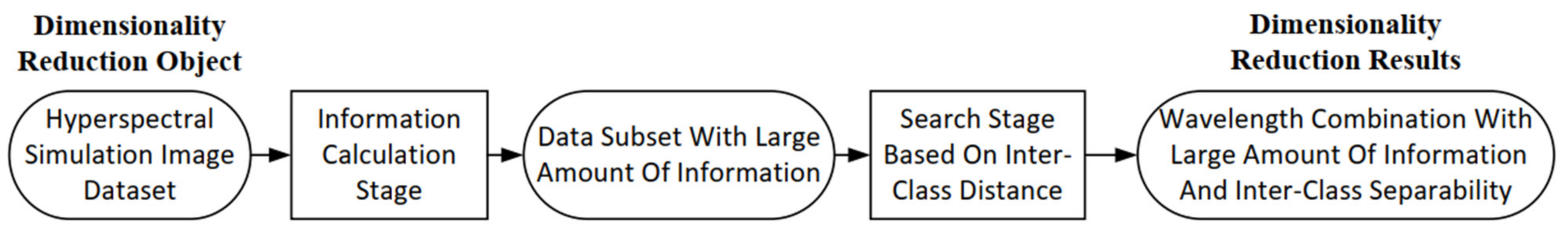
The research ideas of LBI-BPSO can be summarized by the process shown in
Figure 2. The object of DR and classification research is the hyperspectral simulation image dataset established in this paper. Some bands of its samples have close characteristics, and the SNR of the data is controlled by controlling the input noise. In the information calculation stage, the local band index LBI of Equation (3) applied in the IOIF algorithm is used to obtain the information content of all wavelengths, and the wavelength with a larger value is selected according to a certain proportion
to complete the preliminary screening of the spectral wavelength. In the search stage, according to the distance between classes, the binary particle swarm optimization algorithm GA-BPSO with the introduction of a genetic mechanism, is applied to realize the search for the optimal solution of the fitness function
F of Equation (11). The wavelength combination with the largest inter-class distance obtained in the data subset with a large amount of information can determine the DR result that contains both high information content and the largest class distance.
The data sample
of a certain point in the HSI can be expressed as
, and
n is the characteristic dimension of the sample, that is, the number of selected wavelengths. Object points of the same class are represented as
, and
is the number of samples in class
, that is, the number of pixels corresponding to a certain class of ground objects in the image. The pattern average vector of class
is defined as in Equation (8), where
is the number of object categories to be classified. As shown in Equation (9),
represents the Euclidean distance from the center of class
i to the center of class
j:
The sample can be identified by judging the distance between the class center vector and the sample feature vector [
36]. Based on the maximum distance between classes [
36,
37], using the center distance Equations (8) and (9), the objective function
f of the following Equation (10) can be obtained. When the distances between the classes of the samples are larger, the separability between the objects is better. Let the objective function
f be the reciprocal of the sum of the center distances between the classes, and the minimum solution of the function is the best combination of wavelengths.
The main task of this paper is to select a smaller number of wavelengths under the condition of ensuring the classification accuracy. Therefore, this paper defines the fitness function by Equation (11):
where
and
are the number of wavelengths currently selected and target wavelengths, respectively, and
are the penalty coefficients. In order to limit the number of wavelengths selected by the algorithm, when the currently selected number of wavelengths
exceeds the preset target number
, the penalty term
will be used to adjust the fitness state, and finally, a wavelength combination with a smaller number and a larger distance between classes is selected.
The specific implementation steps of the LBI-BPSO method are described in detail in Algorithm 1:
| Algorithm 1: Binary Particle Swarm Optimization with Local Band Index (LBI-BPSO) |
| INPUT: The set of simulation hyperspectral data W, Ground Truth GT, |
| OUTPUT: The global optima |
| INITIALIZATION: |
| Set the parameters: |
| Screening threshold: ; Expected number of wavelengths = 10; |
| Maximum iteration: = 500; Particle swarm size: n = 50; |
| Inertia weight: = 0.6, = 0.1; Learning factor: = 3, = 2; |
| Crossover probability: = 0.8, = 0.3; |
| Mutation probability: = 0.2, = 0.5; |
| Initialize searching space: |
| Randomize the particle to get matrix X and calculate , |
| ITERATION: |
| 1: Calculate and sort the LBI values for all wavelengths by Equation (3) |
| 2: Obtain preliminary wavelength selection by threshold |
| 3: while T < do |
| 4: Update , and , by Equation (11) |
| 5: if T Mod Q1 = 0, then |
| 6: Reduce crossover probability , and increase mutation probability |
| 7: Obtained new particles |
| 8: if optimal than then |
| 9: = |
| 10: end if |
| 11: end if |
| 12: if T Mod Q2 = 0 then |
| 13: Roulette the particle swarm to get a new matrix |
| 14: X = |
| 15: end if |
| 16: Update , and , |
| 17: Update X and by Equations (5)–(7) |
| 18: T = T + 1 |
| 19: end while |
4. Establishment of Simulated HSI Dataset Based on Experimental Measurement
The goal of this section is to build a simulated HSI using samples with similar colors and spectra to test the classification ability of the wavelength selection algorithm LBI-BPSO DR results for similar color samples. Firstly, the multi-point hyperspectral data of the ground objects samples were measured, and these data were regarded as pure pixels in the simulated HSI. Then, the linear mixture model is used to calculate the mixed pixels of each abundance, and these data are used as mixed pixels in the simulated HSI. Based on these pure pixels and mixed pixels, four types of ground objects (three types of vegetation are classified into the same class) HSI can be constructed.
4.1. Experimental Preparation
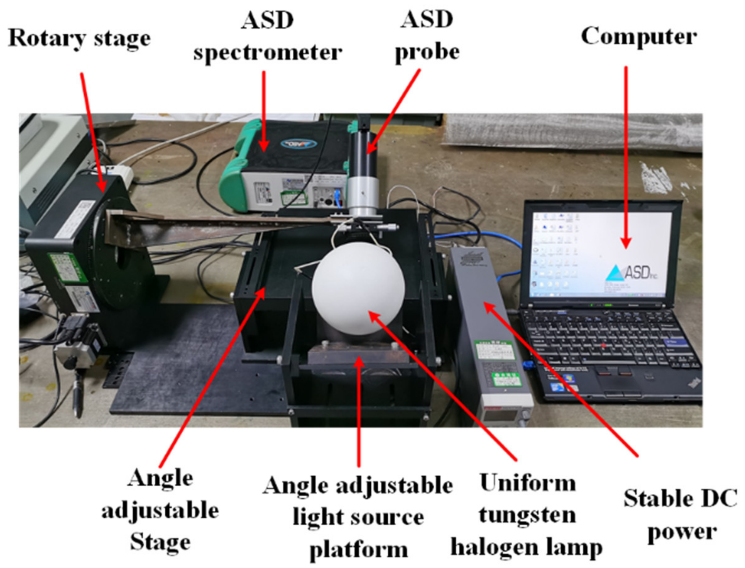
The experimental measurement instrument is a multi-angle spectral reflectance measurement system designed and manufactured by the research group. As shown in
Figure 3, the light source incident angle of the measuring instrument can be adjusted in the range of 0–90°, and the detection angle can be adjusted in the range of 0–90°. The halogen tungsten lamp with a uniform light cover is used as the light source. ASD spectrometer and its optical fiber lens are used as the reflected light-receiving end. The rotary displacement table, the adjustable-angle stage, and the adjustable-angle light source platform are used as the position and angle adjustment mechanism. The computer is used as the data signal processing terminal. The grating dispersive spectrometer ASD (FieldSpec 3, Analytical Spectral Devices) has a detection range of 350–2500 nm, a minimum sampling interval of 1.4 nm, and a minimum spectral resolution of 3 nm. The spectral response range of the polarization module is 430–860 nm and 860–1650 nm.
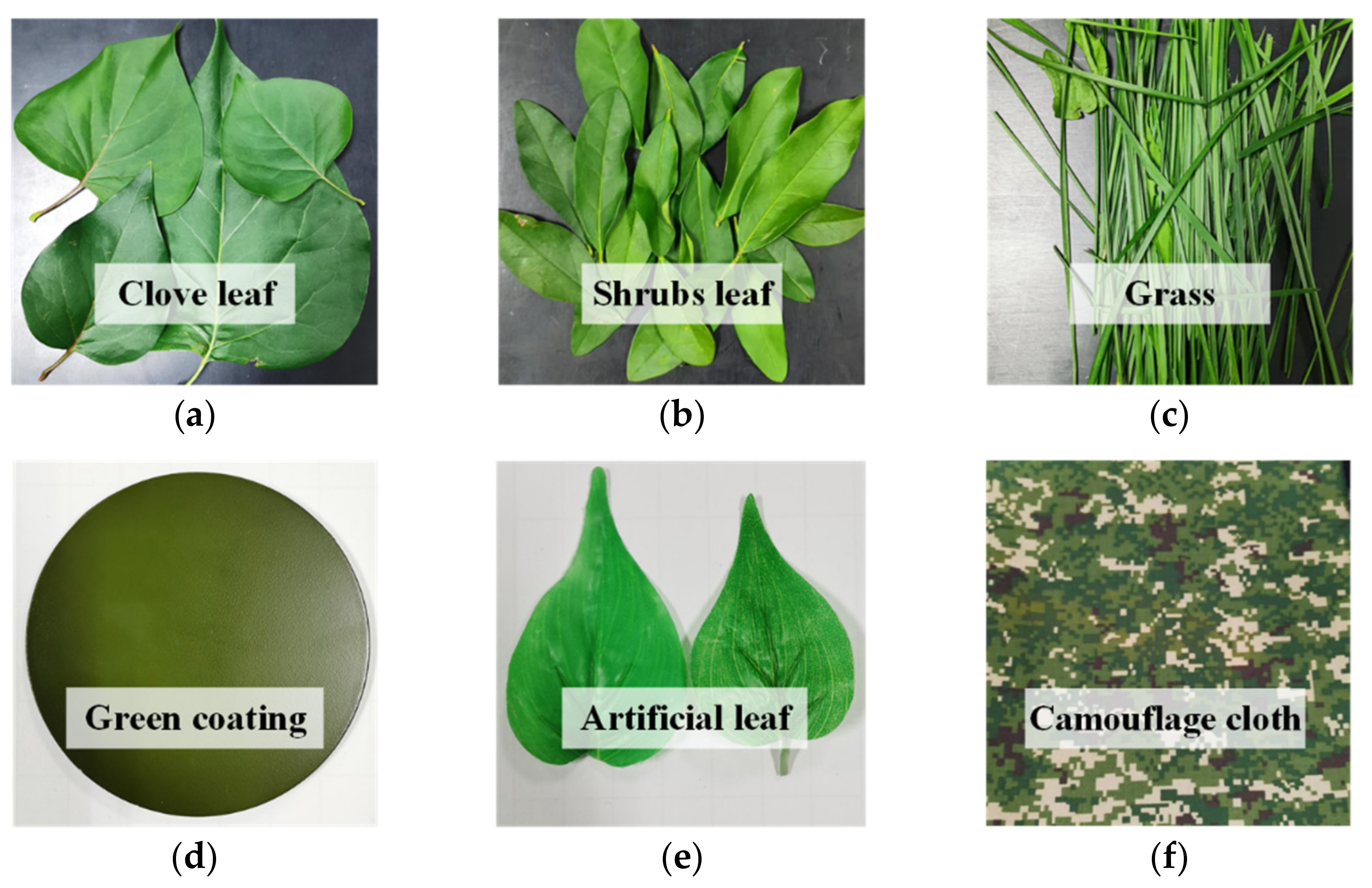
The research samples selected in the experiment are divided into two categories. The first class is vegetation leaf samples: clove leaves, shrub leaves and grass leaves. The second class is artificial objects similar to vegetation: green coatings, artificial leaves and cloth with camouflage patterns. The samples used for data acquisition are shown in
Figure 4: all samples are similar in color and are green. Among them, clove leaves are large, heart-shaped, relatively flat, and smooth, and the leaves are overlapped. Shrub leaves are narrow and oval, curly, with smooth surfaces and overlapping leaves. The grass leaves are thin, narrow, long strip, rough surface, and the leaves are staggered. The surface of the green coating is flat and has a fine texture. The fake leaves are human-made, simulated landscapes, and their surfaces are rough and imitate the leaves’ grain. The camouflage cloth is green as a whole, composed of light green, dark green, brown and yellow.
4.2. Measurement Process and Results
Due to the similarity in the spectral characteristics for some bands of the same color ground objects, a common disadvantage of traditional pixel-by-pixel classifiers based on spectral information is “salt and pepper noise” [
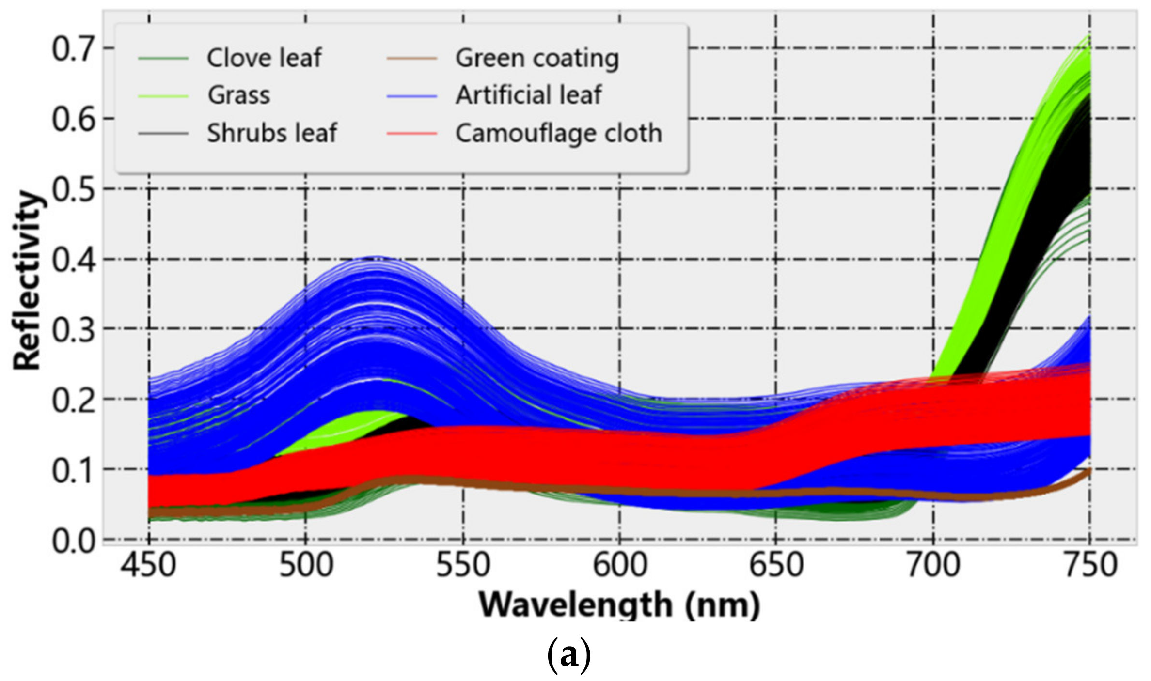
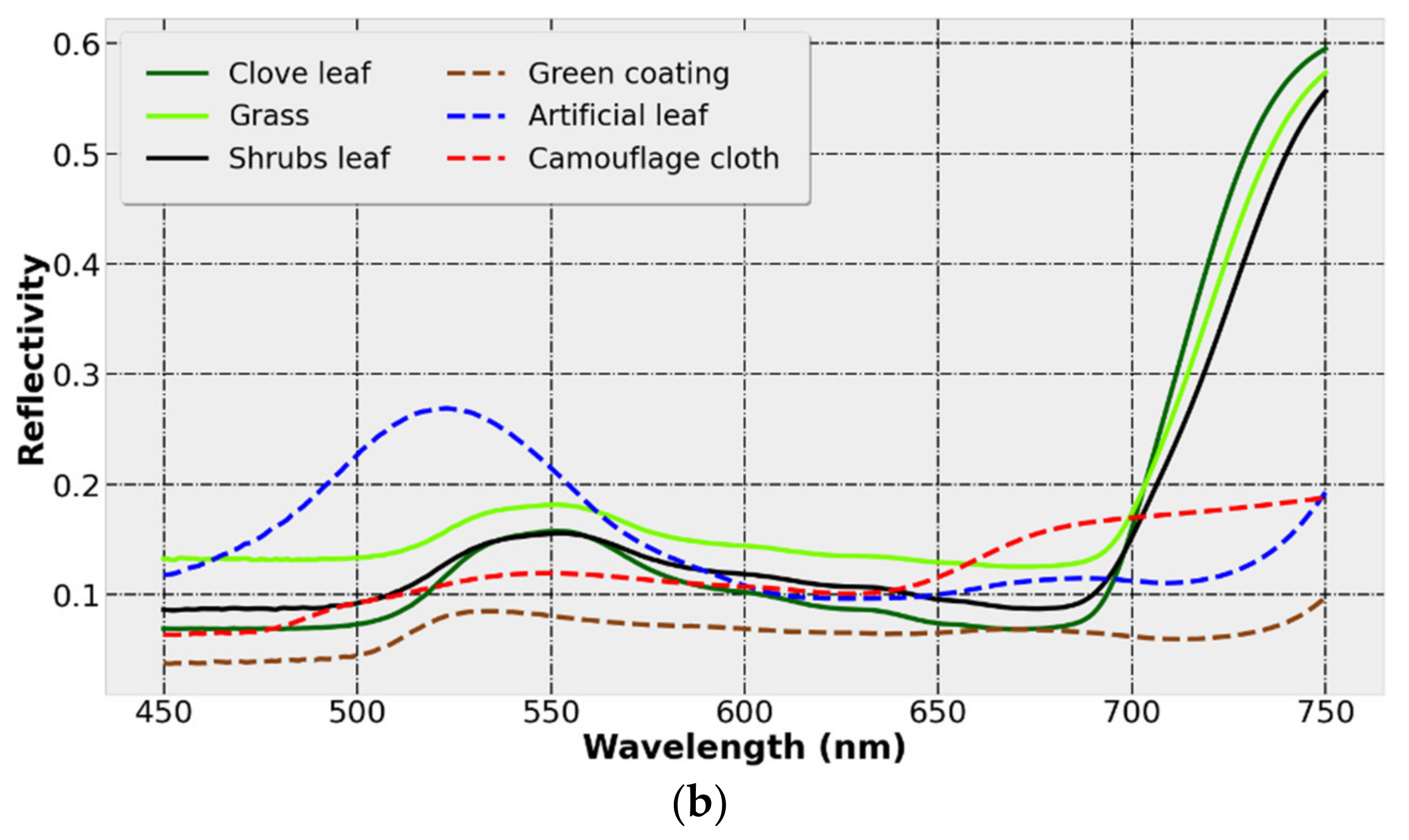
13]. In order to solve the above problems, this paper selects ground objects with similar colors to analyze, process and classify the hyperspectral reflectance data. Spectroscopic measurements were performed in a dark room with vegetation samples placed on an angle-adjustable stage. When measuring the sample, after each measurement point, move the sample by an appropriate distance or replace it with a new sample of the same type and continue to measure until the reflectance data of 240 different points are collected. The acquisition results are shown in
Figure 5a, and
Figure 5b is the average reflectance of the sample in the visible light range. It is worth noting that the purpose of this paper is to propose and verify a DR method that is more suitable for the classification of samples with close spectral characteristics, so the scope of the study is narrowed to the vicinity of the visible light where the spectrum of the ground object is closest. However, in practical applications, in order to give full play to the advantages of the wide spectral response range of HSI, the full range should be used as much as possible to improve the classification accuracy.
Clove leaves, shrub leaves and grass leaves have typical vegetation spectral reflectance characteristics. In the visible light range of 450–750 nm, the reflectance is at a low level. The smaller reflection peak at 550 nm is the “green peak”, and its characteristics are mainly affected by the chlorophyll content of vegetation leaves. After 700 nm, the reflectivity rises rapidly, which is within the red-light range, so it is called the “red edge” phenomenon of vegetation. It is the position where the reflectance of vegetation leaves changes the fastest, which is mainly affected by the structure of vegetation cells.
As shown in
Figure 5a, the spectral numbers of the data samples of the same class show the same curve trend, but there are differences in the values within a certain range. The main reason is the variability of the sample material. For example, the camouflage cloth is composed of four kinds of color blocks (pigments), and the physical performance at different points of the sample is non-uniform, so the spectrum at different points of the same type of objects changes in amplitude. This results in the existence of different degrees of intersection between the spectra of ground objects. On the contrary, the spectrum of green coating with a single material and uniform spraying is very concentrated. Comparing the reflectance curves of the artificial object samples and the vegetation leaves, it can be found that the green artificial objects and the vegetation leaves are generally very similar in the visible light range, showing a lower reflectance spectrum and a reflection peak near 550 nm. After 700 nm, due to the red edge phenomenon of vegetation, the reflectivity of vegetation and human-made objects is significantly different. In practice, there are a large number of mixed pixels in HSIs. The existence of mixed pixels will further enhance the similarity between ground object samples.
4.3. Mixed Pixel Simulation
Section 4.2 carried out independent measurements of reflectivity data for six types of ground objects. However, in practice, due to the low spatial resolution of HSIs, each pixel may contain spectral information of multiple basic objects at the same time. This type of pixel is called “mixed pixel”. The proportion of each type of feature in a mixed pixel is called the “abundance” of a ground object [
38]. The existence of mixed pixels makes the feature space develop in the opposite direction; that is, the intra-class difference becomes larger, and the inter-class coupling becomes stronger, which has a great negative impact on the classification [
39]. In order to verify the influence of mixed pixels on the results obtained by the wavelength selection algorithm, mixed pixel data with an abundance range of 0.75–0.25 and a step size of 0.05 were added to the dataset. Hyperspectral unmixing, that is, extracting basic ground objects from mixed pixels and calculating the abundance of each basic ground object in mixed pixels has become a key preprocessing technique for HSI analysis [
40]. The mixed pixels simulation based on the measured object points hyperspectral data is equivalent to the inverse process of hyperspectral pixel unmixing. The samples reflectance data measured in
Section 4.2 are used as the endmembers’ spectral information to participate in the calculation of the mixed pixels. The existing mixed models mainly include linear models and nonlinear models. For the following two reasons: (a) the linear spectral mixture model has the advantages of simplicity, high efficiency, and well-defined physical meaning; (b) for hyperspectral images with spatial resolution below the meter level, the linear spectral mixing model can better describe the actual spectral mixing phenomenon. In this paper, the Linear Mixing Model (LMM) is selected for the calculation of mixed pixels. It can be described by Equation (12):
where
is the pixel value of the mixed position on the image,
is the abundance of the object sample
i in the pixel
,
is the spectrum of the object sample
i,
is the spectrum of the ground object sample
j, and
e is the Gaussian noise. In this paper,
is the hyperspectral reflectance of the sample measured by ASD.
Figure 6 is a schematic diagram of the mixed reflectance of pixel
i and pixel
j. The pixel abundance is 0.75–0.25, and abundance changes in steps of 0.05.
In order to test the classification performance of the wavelength selected by the DR method under different noises, this paper sets a total of eight non-uniformly spaced signal to noise ratio (SNR) conditions from SNR = 1280 to SNR = 10. The SNRs are (1280, 640, 320, 160, 80, 40, 20, 10).
4.4. Establishment of HSI Dataset
The above shows the simulation of mixed cells and the effect of noise on the spectrum. The following will introduce the process and ideas of designing the dataset.
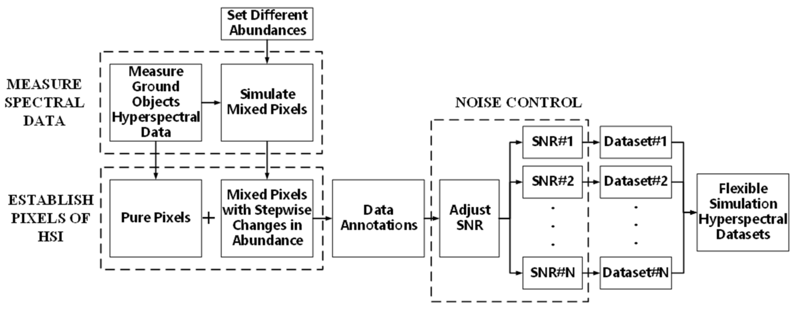
Figure 7 shows the simulation process of HSIs of objects with similar colors in this paper: the spectral reflectance of the measured ground objects is taken as the spectral information for pure pixels, and the gradually changing abundance is set to calculate the mixed pixels, so that the mixed pixels of different abundances in the image can be obtained. After setting different SNRs and labeling the samples, the hyperspectral simulation images of objects with close spectral characteristics can be obtained for the test of DR results. The simulation of HSIs can be performed with a high degree of flexibility by establishing pixel and noise controls.
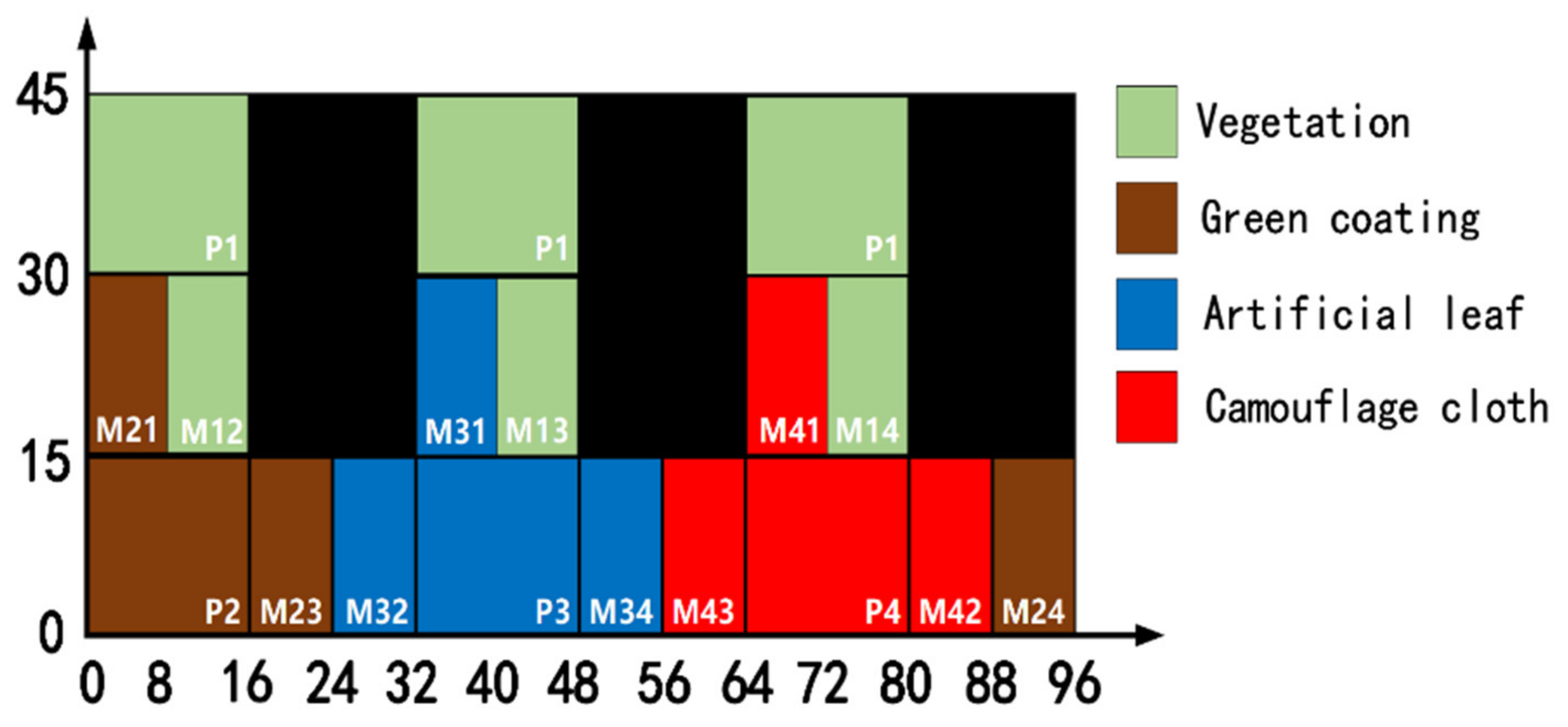
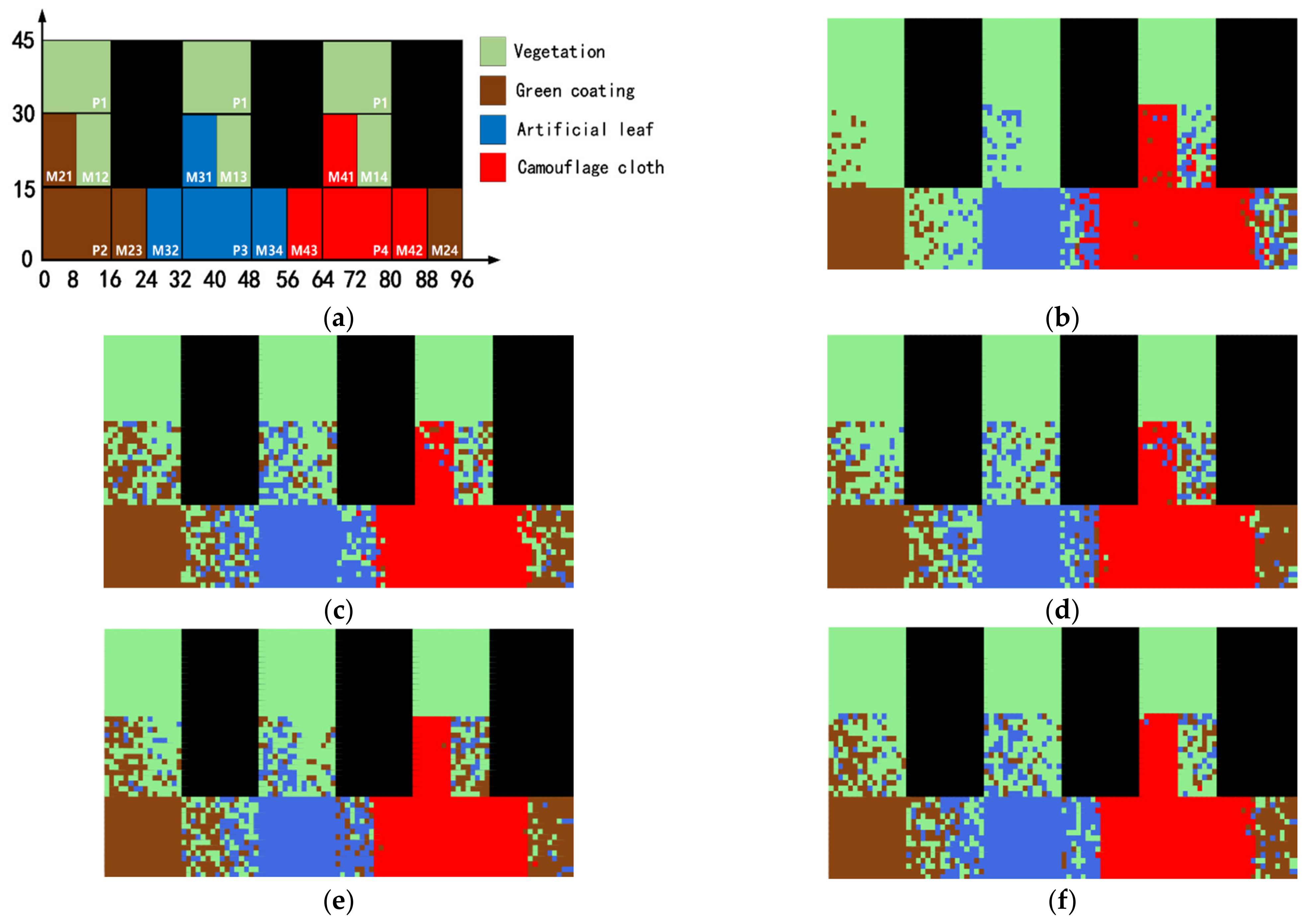
Figure 8 is a schematic diagram of the spatial location of the hyperspectral dataset for 4 types of ground objects, in which the clove leaves, shrub leaves and grasses are classified into one class, and the black area is the blank position of the data. This paper sets 10 abundance ratios: [0.75, 0.70, 0.65, 0.60, 0.55, 0.45, 0.40, 0.35, 0.30, 0.25].
Table 1 shows the meaning of the labels in the spatial schematic diagram. This paper adopts a single-label classification strategy. Mixed cells are also treated as pure cells and assigned a single label for classification, and the object class with greater abundance in the mixed pixel is used as the label of the pixel. Pixel attributes: P represents a pure pixel, followed by numbers representing the feature class label. M represents a mixed pixel; the first number of the mixed pixel represents the feature class with the pixel abundance greater than 0.5. For example, M21 represents a mixed pixel of green coating and vegetation, and the coating abundance is greater than 0.5.
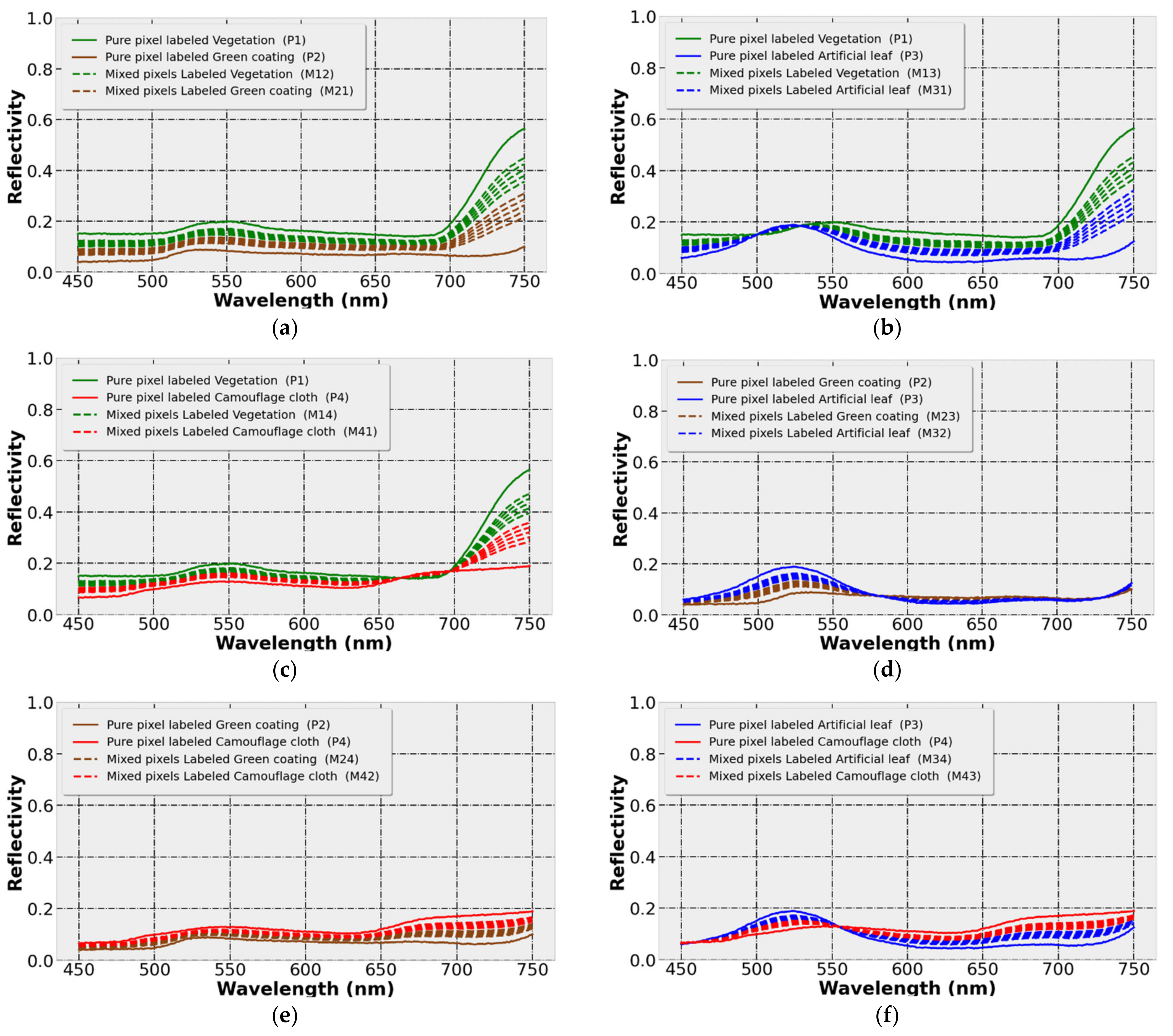
Figure 9 corresponds to
Table 1, which shows the spectral characteristics of the pixels in the hyperspectral simulation image (SNR = 1000). Each subgraph in
Figure 9 consists of a pure pixel randomly selected from each of the two ground objects and their mixed pixels with different abundances. In the figures, different colors represent different classes of ground object pixels, the solid lines represent the pure pixel spectrum, and the dashed lines represent the mixed pixel spectrum.
In
Figure 8, the arrangement direction of mixed pixels radiates outward from pure pixels; that is, for a certain ground object, the pixel with a high abundance value is close to the pure pixel area, and the pixel with a low abundance value is close to the area intersecting with other ground objects. It is worth noting that the pure pixel hyperspectral data in this paper is obtained by ASD. The collection points of ground objects have a randomness, and their texture information was destroyed. In addition,
Figure 8 is only for the convenience of observing the classification results, and this figure can be regarded as a HSI that disrupts the order of pixels inside the object. Since the texture and shape information of the ground objects are not used in the pixel-by-pixel classification in this paper, it has no effect on the classification results.
Above, the sample reflectivity measured in the laboratory was used as the end member to perform a mixed pixel calculation and then establish a simulated HSI. Machine-learning classifiers require a large number of samples for training, and complete data labels are required in the field of hyperspectral remote sensing applications, while manually labeling the HSI dataset is very challenging and requires a lot of work [
41]. This method can not only quantitatively analyze the accuracy of samples with different abundance pixels, but also can easily label all samples, thus eliminating the high cost of manual labeling. In the following, the LBI-BPSO proposed in this paper and the IOIF and GA-BPSO mentioned above will be used to reduce the dimension of the simulated his, respectively. Then, according to these DR results, the simulated HSI is classified, and finally, the classification performance analysis of the wavelengths obtained by the three algorithms for ground objects with close spectral characteristics is completed.
5. Results
The computer operating system of this paper is Windows 10, and the test environment is Python 3.8. In order to analyze the performance of the wavelengths selected by the above DR methods under different noise conditions, the following hyperspectral DR processes are all performed when the additional Gaussian noise is 0.
5.1. Dimension reduction of LBI-BPSO
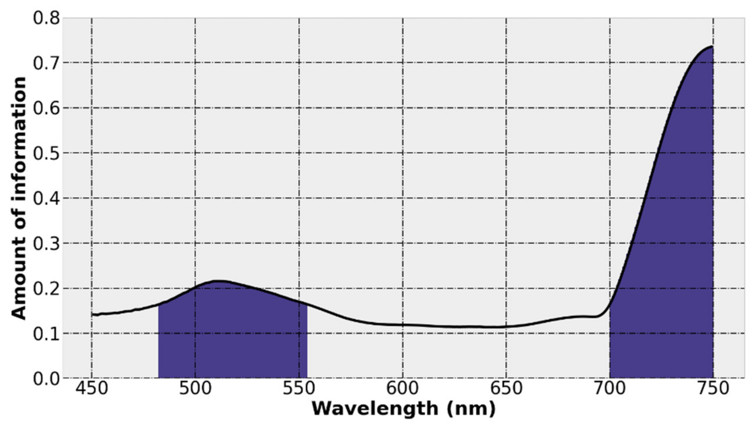
The DR steps of LBI-BPSO are as follows:
(a) Preliminary wavelength selection based on the amount of information calculated by local band index LBI. Set relevant parameters, calculate the local band index (LBI) value of all wavelengths by Equation (3), and then sort out the 60% wavelengths with the largest amount of information as the preliminary selected wavelength subset. The LBI calculation results of all wavelengths are shown in
Figure 10. The black curve is the LBI numerical curve, and the blue shaded part corresponds to the initially screened wavelength subset.
(b) Secondary wavelength selection based on inter-class separability. As described in
Section 2.2, using the binary particle swarm algorithm that introduces the genetic mechanism, the particle velocity
and position
are updated using Equations (5)–(7). The specific steps are described in Algorithm 1. The binary particle swarm is set to the number of iterations
is 500, the number of particles is
n = 50, and the particle dimension is 301, corresponding to the number of original wavelengths, and other specific parameters refer to Algorithm 1. Iterative optimization is performed on the wavelength combination that satisfies the minimum value of the fitness function of Equation (11), proposed by the class center distance, and the search for the wavelength subset with the largest inter-class distance is completed. The optimal result is: (501, 515, 521, 528, 706, 723, 729, 732, 744, 749), 10 wavelengths.
5.2. Results from the Simulation Dataset
Partitioned Relief-F [
42] is also a DR method that selects bands by virtue of the amount of information. It is presented to mitigate the influence of continuous bands on classification accuracy while retaining important information. It determines the amount of information for each band as the importance score through the calculation of “near-hit” and “near-miss”. After all of the bands are partitioned according to the redundancy of the sub-intervals, the bands with the largest scores in each interval are selected to form a DR band set. This method is also used below to compare the LBI-BPSO proposed in this paper. Taking advantage of GA-BPSO, IOIF, Partitioned Relief-F and LBI-BPSO proposed in this paper, respectively, the simulated HSIs established in
Section 4 are used for wavelength selection, and
Table 2 below shows their results. It is worth noting that there is no meaningful order between simulated HSI pixels established in
Section 4; that is, the image data does not have texture information. However, this will not affect the calculation of the correlation coefficient (Equation (2)) and the correlation matrix (Equation (1)), so the IOIF can be used to reduce the dimension of the simulated HSI.
The above wavelengths are used to classify the simulated images of objects with close spectral characteristics obtained in
Section 4. At the same time, the performance of IOIF, GA-BPSO and LBI-BPSO DR results proposed are compared and visualized. Then, we can obtain the comparison of the classification results of the three DR results under the three perspectives of SNR = 1000, mixed pixels with different abundances, and different SNRs. In this paper, stratified sampling is used to randomly select 20% of the samples as the training subset, and the pixel-by-pixel classification is performed by the Support Vector Machine (SVM) classification algorithm with the RBF kernel function.
5.2.1. Analysis for SNR = 1000
The pixel-based evaluations used in HSI classification are the Product’s Accuracy (PA)—that is, the ratio of the number of correctly classified pixels of a certain class to the total number of samples of that class. Overall accuracy (OA): the ratio of the number of correctly classified pixels to the total number of pixels. Average accuracy (AA): the sum of the production accuracy of each class divided by the number of categories. Kappa coefficient: measure the consistency between the classification result map and the real marked map.
Table 3 shows the classification results of the three wavelength selection algorithms on the simulated data set under the conditions of SNR of 1000, and
Figure 11 is the corresponding visual classification diagram. In order to avoid unstable results, each algorithm repeats the dataset 10 times and displays its average accuracy (AVG) and standard deviation (STD). The best results of the three algorithms in the table are highlighted, and SVM is the original wavelength classification result. It can be seen that the SVM classification results using the original 301-dimensional wavelengths only reached a high level for the classification of vegetation and camouflage cloth, while the accuracy of green coating and artificial leaves and the other three classification evaluations of OA, AA and Kappa coefficients are much lower than the results after dimensionality reduction. This demonstrates the necessity of hyperspectral image DR for classification work. Among the four DR methods, the LBI-BPSO method proposed in this paper obtains a smaller number of wavelengths, and is superior to GA-BPSO, IOIF and Partitioned Relief-F in the classification accuracy of various ground objects, OA, AA and Kappa coefficients. Due to the limitation of search performance, the final result of GA-BPSO is 39 wavelengths, and the feature dimension exceeds that of IOIF and LBI-BPSO. From the perspective of classification performance, redundant information leads to a decrease in classification accuracy, so the GA-BPSO algorithm that only uses inter-class separability for optimal combination search is the worst. However, LBI-BPSO makes the search space focus on the characteristic region with a large amount of information through preliminary screening of the wavelengths containing the largest amount of information, and further wavelength selection is carried out with the goal of maximizing the inter-class distance in this region. Finally, LBI-BPSO successfully reduces the initial 301-dimensional feature space to 10-dimensional. The classification effect of LBI-BPSO and Partitioned Relief-F is very close, and LBI-BPSO shows a small advantage. Compared with IOIF, LBI-BPSO classification results show that OA is improved by 2.90%, AA is improved by 2.75%, and Kappa is improved by 3.91. Compared with GA-BPSO, OA is increased by 3.17%, AA is increased by 3.19%, and Kappa is increased by 4.94. The above proves that the LBI-BPSO DR method combining the two DR criteria of information content and inter-class separability is better than IOIF based on information content alone and GA-BPSO considering only inter-class separability in terms of classification effect.
Figure 11 shows the result of the classification visualization. It can be seen from the figure that the samples with incorrect classification are located in the area of mixed pixels, and in the five result diagrams, a large number of mixed pixels are classified as vegetation, which can prove that the mixed spectra of the three types of artificial objects are very similar to the vegetation spectra. Compared with GA-BPSO, IOIF and Partitioned Relief-F, LBI-BPSO has better performance for the classification of mixed vectors. Especially in the edge area of ground objects, that is, for mixed pixels with low abundance values, the result of LBI-BPSO has a more obvious dividing line, and the noise in the mixed pixel area is smaller.
5.2.2. Analysis for Different Abundances
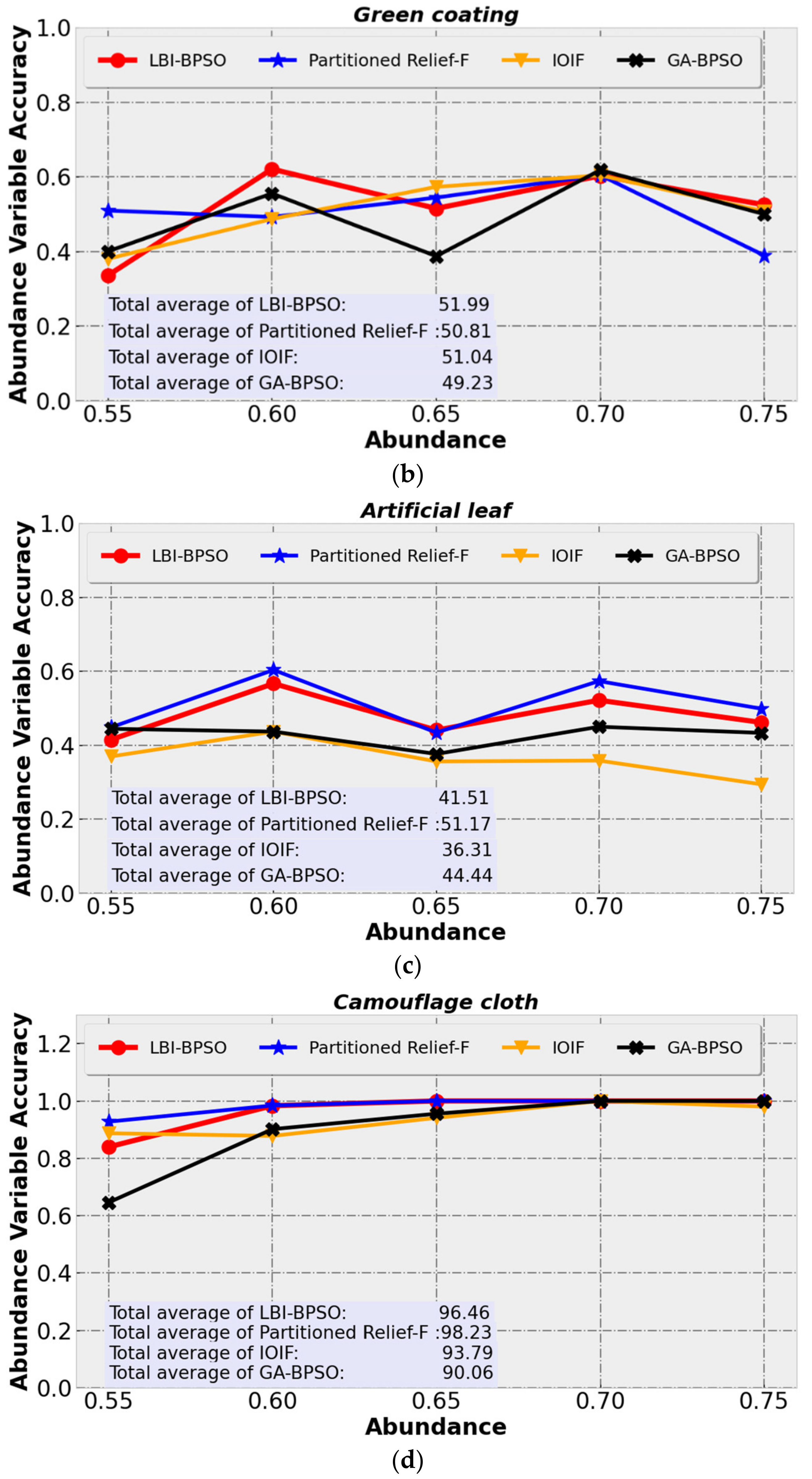
In order to further discuss the influence of different abundances of mixed pixels on the classification accuracy,
Figure 12 shows the correspondence between the classification accuracy of ground objects and the abundance of mixed pixels when the SNR is 1000. In the range of abundance from 0.55 to 0.75, the classification evaluation of mixed pixels according to the PA definition is AVA (Abundance Variable Accuracy) and total average TA. AVA is a variable defined in this paper for the convenience of description. It is obtained from the average value of
N Product’s accuracy PA calculated from mixed pixels of a certain ground object and other
N objects under the specified abundance.
The AVA corresponding to a mixed pixel of the ground object
i with abundance
x (
x > 0.5) is described by Equation (13), where
n is the number of other objects categories except feature
i, and
is the Product’s accuracy of the mixed pixel with object
j when the abundance of object
i is
x. Correspondingly, the total average value TA is the average value of
for the ground object
i at different abundances
x and calculated by Equation (14).
is the number of abundance variables. According to the settings of mixed pixel abundance and single-label classification strategy in
Section 4.3,
is 5 in this paper, as shown by the abscissa in
Figure 12.
Figure 12 shows the performance of the three DR algorithms on AVA and TA for vegetation, green coating, artificial leaves, and camouflage cloth. It can be found that the wavelength results of LBI-BPSO for vegetation, artificial leaf and camouflage cloth have better performance at most abundances, and its TA values are greatly improved compared to IOIF and GA-BPSO. It can be seen that the advantage of LBI-BPSO in distinguishing the green-coating mixed pixels is not significant, but the TA is still at the highest level. Overall, the wavelength selection results of LBI-BPSO showed better classification performance compared to IOIF and GA-BPSO at different abundances.
At the same time, the performance of LBI-BPSO and Partitioned Relief-F are relatively close in both AVA and TA. Interestingly, looking at
Figure 12, it can be found that the accuracy is not positively correlated with the increase in the abundance of target objects. This is due to the similar color and material variability of the samples selected in this paper, and the partial spectra of various ground objects are close. There is, in addition, some high-abundance data obtained by mixing the spectra of the two types of ground objects by Equation (12) just show a higher similarity with the spectrum of the third type of ground objects, resulting in misclassification when the abundance is high. For example,
Figure 12 shows that the green coating and artificial leaf did not increase AVA at an abundance of 0.75. Combined with the classification results in
Figure 11c–e, it can be found that in the mixed areas M23 and M32 of green coating and artificial leaf, there are a large number of pixels in the area close to pure pixels that are classified as vegetation, resulting in a large number of classification noise.
5.2.3. Analysis for Different SNR Conditions
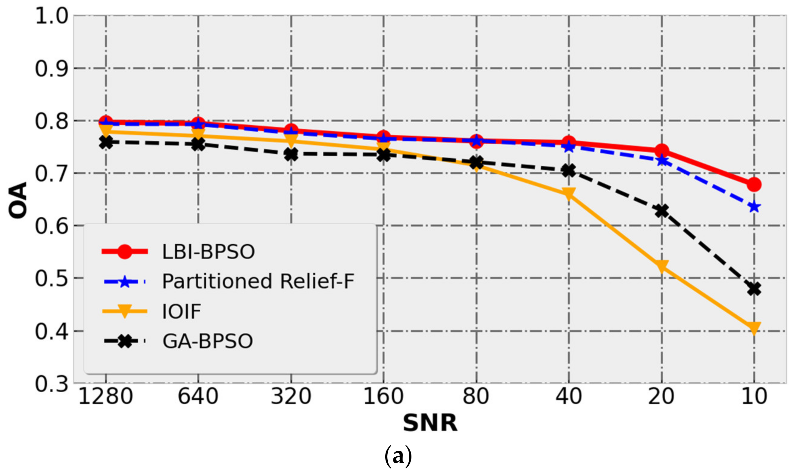
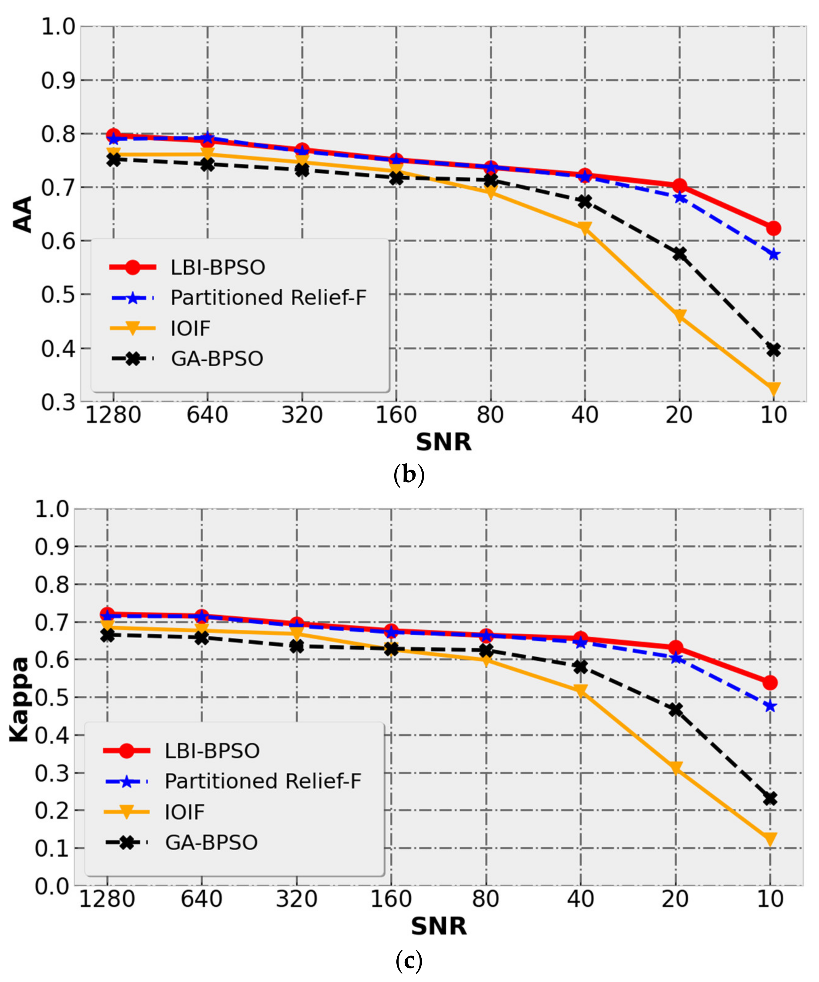
The fault tolerance to noise is an important index to test the performance of the algorithm. The following discusses the tolerance of the wavelengths selected by the LBI-BPSO, IOIF and GA-BPSO algorithms to noise. As shown in
Figure 13, by adjusting the noise term e in Equation (12), the SNRs of the hyperspectral simulation data are gradually reduced from 1280 to 10 for a total of 8 different noise conditions. The values shown in the figure are the average accuracy of 10 repeated runs of the datasets with different SNRs. As described in
Section 4.3, in order to compare the performance of different algorithms under the condition of low SNR more intuitively, the change of SNR is in the form of non-uniform step size.
Table 4 shows the average and standard deviation of the classification result evaluation at the maximum (SNR = 1280), median (SNR = 160) and minimum (SNR = 10) SNRs, and the optimal value in the table is highlighted.
in this table is the relative numerical difference of the evaluation corresponding to the SNR = 1280 and SNR = 10 conditions.
can be calculated by Equation (15),
and
represent the evaluation at SNR = 1280 and SNR = 10, respectively. The smaller the
, the smaller the difference in classification performance of the selected wavelength under the two noise conditions of SNR = 1280 and SNR = 10. Furthermore, the algorithm is less affected by noise. Therefore,
can be used to evaluate the noise tolerance of the wavelength selected by the DR algorithm.
From the classification results of the three DR methods shown in
Figure 13 and
Table 4, it can be found that in terms of the changes in accuracy evaluations with the SNR, LBI-BPSO has always been in a leading position under all standards. Especially in the case of low SNR (SNR < 80), the selected wavelengths of LBI-BPSO can still obtain relatively good classification results. The decreasing trend of classification accuracy for LBI-BPSO is basically the same as that of Partitioned Relief-F, but LBI-BPSO is more dominant under the condition of low SNR. The classification results of IOIF and GA-BPSO showed a significant decline when SNR < 80, and were much lower than LBI-BPSO when SNR = 10. The wavelength selected by IOIF is better than GA-BPSO in the case of high SNR (SNR > 160). In the case of low SNR (SNR < 80), the IOIF classification results show the fastest decline rate, and the obtained evaluation indicators are all lower than GA-BPSO. Continuing to observe
Table 4, it can be found that the relative value difference
of LBI-BPSO is the lowest, and the one of IOIF is the highest. This shows that for the data used in this paper, the wavelength selected only by the amount of information has higher requirements on the SNR. Compared with Partitioned Relief-F, the relative numerical differences
of OA, AA and Kappa coefficients of LBI-BPSO decreased by 4.95%, 5.64% and 8.16, respectively. Compared with IOIF, the
of OA, AA and Kappa coefficients of LBI-BPSO decreased by 33.29%, 35.97% and 57.11, respectively. Compared with GA-BPSO, LBI-BPSO reduces the
of OA, AA and Kappa coefficients by 21.93%, 25.65% and 40.01, respectively. A comparison of the above classification results under different SNR conditions shows that the LBI-BPSO method combining the two wavelength selection criteria of information amount and inter-class separability can still maintain good classification accuracy under the condition of low SNR. Furthermore, LBI-BPSO has stronger tolerance to noise compared with IOIF and Partitioned Relief-F, which perform wavelength selection according to the amount of information and GA-BPSO whose objective function is the inter-class distance.
In sum, the comparison and analysis of the classification results for LBI-BPSO, Partitioned Relief-F, IOIF and GA-BPSO were completed for SNR conditions of 1000, different abundance conditions and different SNR conditions.
6. Conclusions and Future Works
Similar color ground objects dataset. In order to test the DR effect of the wavelength selection method on the hyperspectral dataset with some spectral bands have similarities and save a lot of human resources and the time cost of labeling hyperspectral data. This paper provides a new idea for building hyperspectral datasets by combining laboratory measurement data and using LMM to compute mixed pixels. This dataset is very flexible, maintains the authenticity of the hyperspectral features of the ground objects, and can quantitatively analyze the impact of mixed pixel abundance and data noise on the classification performance, as shown in
Section 5.2.1 and
Section 5.2.2.
A new wavelength selection method is proposed. In order to improve the classification accuracy of HSIs of ground objects with close spectral characteristics. In order to select the wavelength combination with more information, less correlation between bands and good separability between ground objects, a new spectral DR algorithm LBI-BPSO is proposed, which combines the two criteria of information and inter-class separability. The novelty of this study is to propose an improvement on IOIF using inter-class distances. Based on the calculation of the information content by the local band index, the inter-class distance is introduced to measure the inter-class separability of ground objects and a reasonable fitness function is proposed. LBI-BPSO focuses the search direction of the particle swarm in the wavelength region with a large amount of information and can obtain a wavelength combination that takes into account the two DR criteria of greater information amount and better sample separability. Then, comparing four wavelength selection methods LBI-BPSO, Partitioned Relief-F, IOIF and GA-BPSO with the inter-class distance as the objective function, the classification experiments were carried out on the hyperspectral simulation dataset. Furthermore, the performance of the algorithm is analyzed from three perspectives: SNR = 1000, different endmember abundances and different SNR conditions. When the SNR = 1000, the LBI-BPSO classification results are compared with IOIF, the OA is increased by 2.90%, the AA is increased by 2.75%, and the Kappa is increased by 3.91%. The classification effect of LBI-BPSO and Partitioned Relief-F is very close, and LBI-BPSO shows a small advantage. For ground objects of different abundances, LBI-BPSO can achieve the highest overall average score. When the SNR conditions change, LBI-BPSO shows a stronger tolerance to noise.
The relative numerical difference of the classification results are calculated under the two conditions of the highest (SNR = 1280) and the lowest (SNR = 10) SNR. Compared with Partitioned Relief-F, the values of OA, AA and Kappa coefficients of LBI-BPSO decreased by 4.95%, 5.64% and 8.16%, respectively. Compared with IOIF, LBI-BPSO reduces the values of OA, AA and Kappa coefficients by 33.29% and 35.97% and 57.11%, respectively. Compared with GA-BPSO, LBI-BPSO has lower values of OA, AA and Kappa coefficients by 21.93%, 25.65% and 40.01%, respectively. The above experimental results show that the classification performance of the LBI-BPSO method combining the two DR criteria of the amount of information and inter-class separability is better than that of Partitioned Relief-F, IOIF and GA-BPSO with a single criterion. The above advantages are beneficial to technical research on the online classification of live images by preselecting wavelengths with prior information.
Future Works.The use of image simulation based on hyperspectral measured data and the LBI-BPSO DR method can provide a basis for the future development of low-cost multispectral imaging technology. This will be used in the application scenario of online classification of spectrally similar ground object images. This way of thinking can save the high cost of hyperspectral cameras, and uses only a small amount of prior information to complete the establishment of specific ground object simulation data sets. It is used for algorithm testing and related index analysis, and then through the selected wavelength, the online classification technology of multispectral imaging for special objects is developed. The future development goal is to use the wavelength selected by LBI-BPSO to cooperate with the parallel unsupervised classification algorithm to conduct further research on multispectral imaging online detection technology.
Author Contributions
Conceptualization, H.W.; methodology, H.W.; software, H.W.; validation, C.Y., J.Y. and Q.L.; formal analysis, H.W.; resources, C.Y.; data curation, H.W.; writing—original draft preparation, H.W.; writing—review and editing, J.Y.; visualization, H.W.; supervision C.Y., J.Y. and Q.L.; project administration, C.Y.; funding acquisition, C.Y. All authors have read and agreed to the published version of the manuscript.
Funding
This research was funded by the National Key Research and Development Program of China under Grant 2016YFF0103603; in part by the Technology Development Program of Jilin Province, China under Grant 20180201012GX; in part by the National Natural Science Foundation of China (NSFC) under Grant 61627819, Grant 61727818, Grant 6187030909, and Grant 61875192, Grant 61805235; and in part by the STS Project of Chinese Academy of Sciences under Grant KFJ-STS-SCYD-212, Grant KFJ-STS-ZDTP-049, and Grant KFJ-STS-ZDTP-057.
Institutional Review Board Statement
Not applicable.
Informed Consent Statement
Not applicable.
Data Availability Statement
Data sharing is not applicable.
Conflicts of Interest
The authors declare no conflict of interest.
References
- Peddinti, V.S.S.; Mandla, V.R.; Mesapam, S.; Kancherla, S. Simulation of hyperspectral image with existing Sentinel and AVIRIS data using distance functions. Arab. J. Geosci. 2021, 14, 1689. [Google Scholar] [CrossRef]
- Li, N.; Wang, Z. Spatial Attention Guided Residual Attention Network for Hyperspectral Image Classification. IEEE Access 2022, 10, 9830–9847. [Google Scholar] [CrossRef]
- Hughes, G.F. On the mean accuracy of statistical pattern recognizers. IEEE Trans. Inf. Theory 1968, 14, 55–63. [Google Scholar] [CrossRef] [Green Version]
- Huang, W.; Huang, Y.; Wang, H.; Liu, Y.; Shim, H.J. Local Binary Patterns and Superpixel-based Multiple Kernels for Hyperspectral Image Classification. IEEE J. Sel. Top. Appl. Earth Obs. Remote Sens. 2020, 13, 4550–4563. [Google Scholar] [CrossRef]
- Wang, Z.Y.; Xia, Q.M.; Yan, J.W.; Xuan, S.Q.; Su, J.H.; Yang, C.F. Hyperspectral Image Classification Based on Spectral and Spatial Information Using Multi-Scale ResNet. Appl. Sci. 2019, 9, 4890. [Google Scholar] [CrossRef] [Green Version]
- Tripathi, P.; Garg, R.D. Comparative Analysis of Singular Value Decomposition and Eigen Value Decomposition Based Principal Component Analysis for Earth and Lunar Hyperspectral Image. In Proceedings of the 2021 11th Workshop on Hyperspectral Imaging and Signal Processing: Evolution in Remote Sensing (WHISPERS), Amsterdam, The Netherlands, 24–26 March 2021; pp. 1–5. [Google Scholar]
- Bao, Y.; Mi, C.; Wu, N.; Liu, F.; He, Y. Rapid Classification of Wheat Grain Varieties Using Hyperspectral Imaging and Chemometrics. Appl. Sci. 2019, 9, 4119. [Google Scholar] [CrossRef] [Green Version]
- Cai, W.; Guan, G.; Pan, R.; Zhu, X.; Wang, H. Network linear discriminant analysis. Comput. Stat. Data Anal. 2017, 117, 32–44. [Google Scholar] [CrossRef]
- Li, N.; Zhou, D.; Shi, J.; Wu, T.; Gong, M. Spectral-Locational-Spatial Manifold Learning for Hyperspectral Images Dimensionality Reduction. Remote Sens. 2021, 13, 2752. [Google Scholar] [CrossRef]
- Öztürk, Ü.; Yılmaz, A. An Optimization Technique for Linear Manifold Learning-Based Dimensionality Reduction: Evaluations on Hyperspectral Images. Appl. Sci. 2021, 11, 9063. [Google Scholar] [CrossRef]
- Cai, F.; Guo, M.-X.; Hong, L.-F.; Huang, Y.-Y. Classification of Hyperspectral Images Based on Supervised Sparse Embedded Preserving Projection. Appl. Sci. 2019, 9, 3583. [Google Scholar] [CrossRef] [Green Version]
- Subudhi, S.; Patro, R.; Biswal, P.K.; Dell’Acqua, F. Superpixel-Based Singular Spectrum Analysis for Effective Spatial-Spectral Feature Extraction. Appl. Sci. 2021, 11, 10876. [Google Scholar] [CrossRef]
- Lishuan, H. Study of Dimensionality Reduction and Spatial-spectral Method for Classification of Hyperspectral Remote Sensing Image. Doctoral Dissertation, China University of Geosciences, Beijing, China, October 2018. [Google Scholar]
- Song, X.-F.; Zhang, Y.; Gong, D.-W.; Sun, X.-Y. Feature selection using bare-bones particle swarm optimization with mutual information. Pattern Recognit. 2021, 112, 107804. [Google Scholar] [CrossRef]
- Medjahed, S.A.; Saadi, T.A.; Benyettou, A.; Ouali, M. Gray wolf optimizer for hyperspectral band selection. Appl. Soft Comput. 2016, 40, 178–186. [Google Scholar] [CrossRef]
- Li, S.; Wu, H.; Wan, D.; Zhu, J. An effective feature selection method for hyperspectral image classification based on genetic algorithm and support vector machine. Knowl.-Based Syst. 2011, 24, 40–48. [Google Scholar] [CrossRef]
- Wang, M.; Wu, C.; Wang, L.; Xiang, D.; Huang, X. A feature selection approach for hyperspectral image based on modified ant lion optimizer. Knowl.-Based Syst. 2019, 168, 39–48. [Google Scholar] [CrossRef]
- Kennedy, J.; Eberhart, R. Particle swarm optimization. In Proceedings of ICNN’95—International Conference on Neural Networks, Perth, Australia, 27 November–1 December 1995; IEEE: New York, NY, USA, 1995; Volume 4, pp. 1942–1948. [Google Scholar]
- Huang, F.; Ling, J.; Shi, A.; Xu, L. A Band Selection Method for Hyperspectral Images Using Choquet Fuzzy Integral. J. Comput. 2010, 5, 1019–1026. [Google Scholar] [CrossRef]
- Sun, X.; Zhang, H.; Xu, F.; Zhu, Y.; Fu, X. Constrained-target band selection with subspace partition for hyperspectral target detection. IEEE J. Sel. Top. Appl. Earth Obs. Remote Sens. 2021, 14, 9147–9161. [Google Scholar] [CrossRef]
- Hu, L.; Qun, W.; Xing, T. An Algorithm of Improved Optimum Index Factor Band Selection from Hyperspectral Remote Sensing Image. In Proceedings of the 2018 International Conference on Physics Computing and Mathematical Modeling (PCMM 2018), Shanghai, China, 15–16 April 2018; pp. 193–198. [Google Scholar] [CrossRef]
- Chavez, P.S. Statistical method for selecting Landsat MSS ratios. J. Appl. Photogr. Eng. 1982, 8, 23–30. [Google Scholar]
- Akpan, U.I.; Starkey, A. Review of classification algorithms with changing inter-class distances. Mach. Learn. Appl. 2021, 4, 100031. [Google Scholar] [CrossRef]
- Wang, H.Y.; Wang, J.S.; Zhu, L.F. A new validity function of FCM clustering algorithm based on intra-class compactness and inter-class separation. J. Intell. Fuzzy Syst. 2021, 40, 12411–12432. [Google Scholar] [CrossRef]
- Du, Q.; Chang, C.I. A linear constrained distance-based discriminant analysis for hyperspectral image classification. Pattern Recognit. 2001, 34, 361–373. [Google Scholar] [CrossRef]
- Kennedy, J.; Eberhart, R.C. A discrete binary version of the particle swarm algorithm. In Proceedings of the 1997 IEEE International Conference on Systems, Man, and Cybernetics. Computational Cybernetics and Simulation, Orlando, FL, USA, 12–15 October 1997; IEEE: New York, NY, USA, 1997; Volume 5, pp. 4104–4108. [Google Scholar]
- Liu, Y.; Tian, X.; Zhan, H. Research on Inertia Weight Control Method of Particle Swarm Optimization Algorithm. J. Nanjing Univ. Nat. Sci. Ed. 2011, 47, 364–371. [Google Scholar]
- Chen, M.; Jia, J.; Han, Q. Research on Inertia Weight Decreasing Strategy of Particle Swarm Optimization Algorithm. J. Xi’an Jiaotong Univ. 2006, 40, 53–56. [Google Scholar]
- Zhang, Z.; Wei, P.; Li, Y.; Lan, J.; Xu, P.; Chen, B. Improved Feature Selection Algorithm for Particle Swarm Joint Tabu Search. J. Commun. 2018, 39, 60–68. [Google Scholar]
- Zhang, Q.; Xue, S. An improved multi-objective particle swarm optimization algorithm. In International Symposium on Intelligence Computation and Applications; Springer: Berlin/Heidelberg, Germany, 2007; pp. 372–381. [Google Scholar]
- Mirjalili, S.; Lewis, A. S-shaped versus V-shaped transfer functions for binary particle swarm optimization. Swarm Evol. Comput. 2013, 9, 1–14. [Google Scholar] [CrossRef]
- Roy, C.; Das, D.K. A hybrid genetic algorithm (GA)–particle swarm optimization (PSO) algorithm for demand side management in smart grid considering wind power for cost optimization. Sādhanā 2021, 46, 101. [Google Scholar] [CrossRef]
- Molaei, S.; Moazen, H.; Najjar-Ghabel, S.; Farzinvash, L. Particle swarm optimization with an enhanced learning strategy and crossover operator. Knowl.-Based Syst. 2021, 215, 106768. [Google Scholar] [CrossRef]
- Chen, Y.; Li, L.; Xiao, J.; Yang, Y.; Liang, J.; Li, T. Particle swarm optimizer with crossover operation. Eng. Appl. Artif. Intell. 2018, 70, 159–169. [Google Scholar] [CrossRef]
- Zhao, W.; Wang, Y.; Zhang, Z.; Wang, H. Multicriteria ship route planning method based on improved particle swarm optimization–genetic algorithm. J. Mar. Sci. Eng. 2021, 9, 357. [Google Scholar] [CrossRef]
- Zhang, T.; Hu, J.; Fan, S.; Yu, Y. CDCNN: A Model Based on Class Center Vectors and Distance Comparison for Wear Particle Recognition. IEEE Access 2020, 8, 113262–113270. [Google Scholar] [CrossRef]
- Li, C.; Liu, Z.; Ren, J.; Wang, W.; Xu, J. A Feature Optimization Approach Based on Inter-Class and Intra-Class Distance for Ship Type Classification. Sensors 2020, 20, 5429. [Google Scholar] [CrossRef]
- Song, M. Research on sub-pixel mapping method of hyperspectral remote sensing image based on multi-objective optimization theory. Ph.D. Thesis, Wuhan University, Wuhan, China, May 2021. [Google Scholar]
- Zhang, J.; Wang, Y.; Fang, S. Multi-label hyperspectral image classification. J. Image Graph. 2020, 25, 568–578. [Google Scholar]
- Yuan, J.; Zhang, Y.; Gao, F. An overview on linear hyperspectral unmixing. J. Infrared Millim. Waves 2018, 37, 553–571. [Google Scholar]
- Ahmad, M. Ground truth labeling and samples selection for hyperspectral image classification. Optik 2021, 230, 166267. [Google Scholar] [CrossRef]
- Ren, J.; Wang, R.; Liu, G.; Feng, R.; Wang, Y.; Wu, W. Partitioned relief-F method for dimensionality reduction of hyperspectral images. Remote Sens. 2020, 12, 1104. [Google Scholar] [CrossRef] [Green Version]
| Publisher’s Note: MDPI stays neutral with regard to jurisdictional claims in published maps and institutional affiliations. |
© 2022 by the authors. Licensee MDPI, Basel, Switzerland. This article is an open access article distributed under the terms and conditions of the Creative Commons Attribution (CC BY) license (https://creativecommons.org/licenses/by/4.0/).


