Article

A Human Location Prediction-Based Routing Protocol in Mobile Crowdsensing-Based Urban Sensor Networks

Department of Electrical, Electronic and Computer Engineering, University of Ulsan, Ulsan 44610, Korea
*
Author to whom correspondence should be addressed.
Appl. Sci. 2022, 12(8), 3898; https://doi.org/10.3390/app12083898
Submission received: 19 February 2022 / Revised: 4 April 2022 / Accepted: 8 April 2022 / Published: 12 April 2022
(This article belongs to the Section Electrical, Electronics and Communications Engineering)

Abstract

:
Mobile crowdsensing (MCS) has recently emerged as an urban-sensing paradigm that takes advantage of smartphone sensing capabilities and user mobility. A major challenge in mobile crowdsensing-based urban sensor networks is how to efficiently transfer data from sensors to the sink (e.g., the server center). Therefore, this study proposes a human location prediction-based routing protocol (HLPRP) in such networks. Specifically, a human location prediction (HLP) model is designed to estimate the location of mobile nodes. The proposed HLP model is based on a recurrent neural network with long short-term memory cells. The movement history of each person is used in the HLP model to predict their future locations. Experimental results on real traces are used to validate the proposed HLP model. Then, using predicted location information from the HLP model, packet delivery predictability is obtained. Packet delivery predictability represents the possibility that a node will deliver a packet to its destination and is used to select optimal relay nodes to maximize the packet delivery ratio, minimize the packet delivery cost, and reduce delivery latency. In addition, the proposed routing protocol considers social strength for relay selection. To evaluate the HLPRP, we conduct simulations and compare results with other routing protocols, showing that the HLPRP can outperform existing protocols.

1. Introduction

Mobile crowdsensing (MCS) [1,2,3] is an approach to data collection based on the widespread use of mobile devices with sensor capabilities (e.g., smartphones, smartwatches, and tablets). Mobile users can collect and share a lot of relevant data from their smart devices. MCS has been used in a variety of urban-sensing applications, such as environmental monitoring [4,5], intelligent transportation systems [6,7], and public safety [8]. In this work, MCS-based urban sensor networks are considered with the MCS as the main sensing paradigm for a multi-access edge computing environment and additional static sensors. This model includes a server center, edge nodes, sensors, and mobile users. Mobile users collect data using sensors in their smart devices. Sensors are deployed in certain places to capture data such as air pollution, radioactivity, noise level, and humidity. Edge nodes are placed in particular locations to gather and preprocess data from sensors and mobile users. Then, edge nodes send processed data to the server center, where it is used for a variety of applications. The server center communicates with edge nodes using an infrastructure-based wired or wireless network. For communication between other components (i.e., edge nodes, sensors, and mobile users), the wireless interfaces (e.g., Bluetooth 5.0) are used without the need for an infrastructure network. The primary benefit of this network is that it is cost-effective. However, owing to user mobility, the connections between nodes are intermittent, making data collection difficult. That requires an effective routing protocol to transfer data between edge nodes, sensors, and mobile users.
A lot of routing protocols for transferring data between edge nodes, sensors, and mobile users have been studied [9,10,11,12,13,14,15]. For example, several routing methods use the flooding strategy [9,10]. However, with the flooding strategy, messages are immediately spread when there are contacts between nodes. As a result, those routing protocols consume a lot of resources and have a high network overhead ratio. To minimize overhead, the number of replications was limited in [11]. Nevertheless, this routing protocol did not take into account optimal relay selection. Therefore, low mobility nodes can be selected to forward messages, resulting in a low packet delivery ratio and long delivery latency. In [12,13,14], nodes that recently encountered the destination are preferred for selection as relay nodes. However, in a real context, two individuals may often meet in the present moment, but their next meeting may occur in the distant future. For example, family members frequently interact in the morning but do not meet until the evening. As a result, the optimal relay nodes may not be chosen, and those routing protocols may not achieve high network performance.
In [15], a day is divided into time slots, and the meeting probability between nodes is estimated for each time slot based on encounter histories. If two nodes frequently encountered each other in a certain time slot in the past, they will have a high probability of meeting in that time slot in the future. In other words, the estimated value of the meeting probability between two nodes in a time slot only depends on the statistics of their encounters in that time slot in the past. However, in the real context, meeting probability in a certain time slot can be affected by encountering information in other time slots during the day. Therefore, using statistics on encounters between nodes may not be the best method for predicting meeting probability. As a result, high network performance might not be obtained when using the meeting probability for relay selection.
To address those issues, in this paper, we propose a human location prediction (HLP)-based relay selection model that uses a recurrent neural network (RNN) with long short-term memory (LSTM) cells [16]. RNNs have emerged as a potential model for processing sequential data in a variety of applications, such as time-series prediction, video tagging, speed recognition, and generating image descriptions. However, RNNs suffer from both gradient vanishing and gradient explosion problems with long sequences of input. Therefore, we use LSTMs to overcome the problem. A RNN with LSTM cells contains states that enable them to process variable-length sequences of input. In other words, those states are capable of capturing historical information from an arbitrary length of the context window. In the proposed HLP model, the movement histories of mobile users in current and previous time slots (e.g., mobile users’ identities, mobile users’ positions, the time slot of the day, the day of the week) are used to predict their positions in the next several time slots with high accuracy. Note that edge nodes are deployed in specific locations in MCS-based urban sensor networks, and packet destinations are among the edge nodes. Packet delivery predictability is calculated based on the probability that a mobile node will visit an edge node’s position. A mobile node with a high probability of meeting an edge node during a certain time slot has a high value for packet delivery predictability to that edge node. Packet delivery predictability represents the possibility that a node will deliver a packet to its destination.
In addition, the social relationships between nodes are taken into account based on their movement histories. Two nodes have high social strength if they interact frequently over a long period of time. Finally, the human location prediction-based routing protocol (HLPRP) for mobile crowdsensing-based urban sensor networks is designed based on a HLP-based relay selection and social strengths between nodes. More specifically, the proposed routing algorithm has two phases. When a packet is generated, the proposed forwarding algorithm quickly spreads a limited number of copies of the packet throughout the network in the first phase. Then, optimal relay nodes are selected to forward the packet based on packet delivery predictability and social strength in the second phase.
To evaluate the performance of the HLPRP, the proposed HLP model is first trained and tested using a University at Buffalo (UB) dataset [17]. Then, we compare the HLPRP against other routing protocols. According to the obtained results, the HLPRP can outperform existing protocols in terms of delivery cost ( D C ), packet delivery latency ( P D L ), and packet delivery ratio ( P D R ). In summary, this study has the following main contributions.
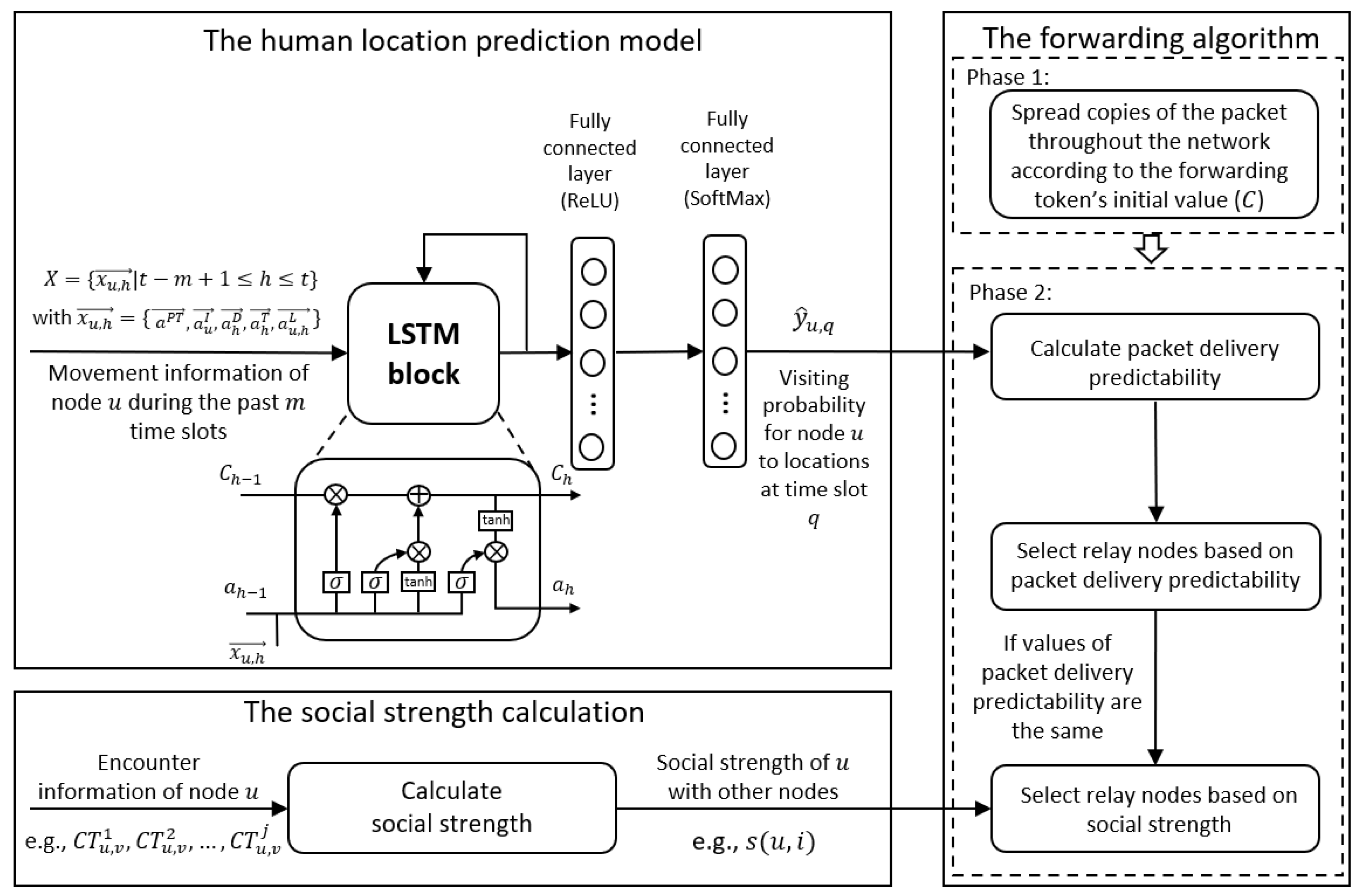
  • First, we design a RNN-based model for human location prediction. Using the predicted information, the packet delivery predictability is proposed and used for relay selection.
  • Second, we propose a forwarding algorithm based on the HLP and social strength. There are two phases in the proposed forwarding algorithm. In the first phase, a limited number of copies of the packet are quickly spread throughout the network. In the second phase, packet delivery predictability and social relationships are used to select optimal relay nodes, with the goal of maximizing the P D R , minimizing the D C , and reducing the P D L .
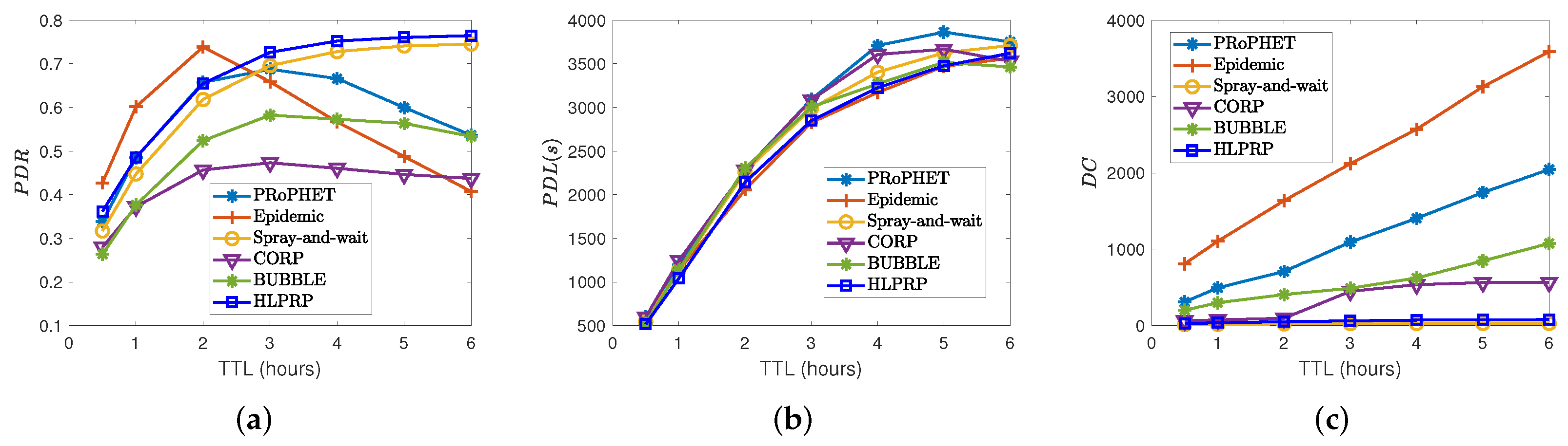
  • Third, using the UB dataset [17], we conduct various experiments to validate the proposed routing protocol. The D C , P D L , and P D R are used to evaluate network performance. The simulation results demonstrate that the HLPRP can outperform existing routing protocols.
The rest of this paper is organized as follows. First, Section 2 discusses related work. Then, the network model and problem definition are presented in Section 3. Section 4 describes the proposed routing protocol in more detail. In Section 5, simulation results from the proposed routing protocol are evaluated. Finally, the conclusion is presented in Section 6.

2. Related Work

In this section, the existing routing protocols for MCS-based urban sensing are presented and compared with the proposed routing protocol.
In early work, the flooding technique was used in a number of routing protocols [9,10]. Messages are spread throughout the network as widely as possible under those protocols. There is a high D C because nodes continually replicate messages for newly found contacts that have not yet processed a copy of the messages. To reduce the D C , several studies [11,18] restricted the number of times a message was replicated. However, a method to quickly spread copies of packets throughout the networks was not considered in those protocols. To overcome this issue in our routing protocol, a forwarding token is used and updated based on degree centrality. The node with a greater degree of centrality will be assigned a larger value for the forwarding token. That helps the rapid spread of packets into the network and minimizes P D L . Moreover, those other routing protocols did not take into account the importance of selecting optimal relay nodes. As a result, messages could be forwarded to nodes that rarely interact with the destination. That results in a low P D R and high latency. To address this issue, the HLPRP executes relay selection in order to choose the optimal nodes for packet relay.
Numerous studies have been proposed for relay selection [19,20,21,22,23,24,25,26]. For example, in [19,20], the physical locations of nodes were used for relay selection. Specifically, the distances between nodes were used to determine which node should be chosen as a forwarding node. It is preferable to choose a node that is closer to the destination. The work in [21] tried to improve the spray-and-wait routing protocol [11] by taking into account node performance. Specifically, a node with a higher capability receives more copies of messages during the spray phase. Then, in the wait phase, it not only delivers packets to their destinations but also forwards them to higher capability nodes. However, the metrics considered in those routing protocols (e.g., node capability and distance between nodes) do not accurately represent the chance of a node encountering the destination in the future. As a result, the probability of sending messages to the destination is still low. Unlike those studies, our work proposes a human location prediction model based on a RNN to estimate whether a node will meet or not meet the destination in the future. Then, optimal relay nodes can be selected.
To improve the relay selection method, a number of routing protocols have been proposed based on social communities and the properties of nodes. For instance, in [25], nodes are divided into communities, and packets were only forwarded to nodes belonging to the destination’s community. In the BUBBLE Rap routing protocol [26], network communities were determined by K-clique algorithm. The local ranking of a node refers to the node’s betweenness centrality in its community, whereas the global ranking refers to the node’s betweenness centrality with all other nodes in the network. A message is routed to nodes that have a higher ranking. Until a node in the destination’s community is found, global ranking is used. After that, local ranking is used. However, forming communities is challenging in those routing protocols since a node must have all the information on all other nodes. In [22,23,24], relay selection was based on centrality metrics. Specifically, packets were routed to nodes with a greater centrality value. Nevertheless, forwarding a large number of messages to central nodes results in congested traffic and long delays around those nodes. To address these problems, the HLPRP chooses nodes with a high probability of meeting the destination and a close relationship with the destination, rather than choosing a node with a high probability of interacting with all other nodes in the network. In other words, the HLPRP selects specific relays for each destination. Based on that, traffic congestion and delays can be avoided.
Based on nodes’ encounter histories, a number of routing protocols were proposed [12,13,27,28,29,30]. In [13,27], delivery predictability was proposed based on encounter history. This value indicates how likely a node will be able to send a message to the destination. If a node encounters another node with a higher value for delivery predictability to the destination, the node replicates the message. Under [12,28,29,30], delivery predictability was also used for relay selection. Furthermore, those protocols control and limit the number of replications to reduce the D C . The community-based opportunistic routing protocol (CORP) [14] considers both delivery predictability and network communities. First, network communities are discovered, and then a communication probability value between two communities is defined. In particular, if nodes in one community often encounter nodes from another community, the two communities have a high community probability with each other. Then, a node with high delivery predictability is preferred as a relay node if the destination community and the source community are the same; otherwise, it chooses nodes in the community of the destination and nodes in communities with a greater community probability with the destination community. These routing protocols’ metrics (e.g., delivery predictability and community probability) could represent how frequently two nodes have interacted in the recent past. However, they cannot estimate when the two nodes will encounter each other in the future. Two nodes may interact frequently in the present, but their next contact may happen in the distant future. For example, two students frequently meet each other in the morning when they attend the same class but do not meet again until the next morning. Therefore, the delivery predictability and community probability might be high at present, but the two nodes might not meet in the near future. As a result, optimal relay nodes might not be selected, and the routing protocols are unable to achieve high performance.
In [15], a day was divided into time slots, and then, based on nodes’ encounter histories, the meeting probability between nodes was estimated for each time slot. If two nodes have met frequently in a time slot in the past, they will have a high probability of meeting again in that time slot in the future. The estimated value of the meeting probability between two nodes in a time slot only depends on the statistics of their previous encounters in that time slot. Nevertheless, in the real world, the meeting probability in a time slot can be influenced by encountering information from other time slots during the day. Therefore, using statistics on node encounters may not be the best method for estimating meeting probability. As a result, high network performance might not be obtained when using only meeting probability for relay selection. Our proposed routing protocol can overcome this problem by developing and using human location prediction-based relay selection based on a RNN and LSTM cells. The prediction model takes the information of mobile users in current and previous time slots (e.g., mobile users’ identity, mobile users’ positions, the time slot of the day, the day of the week) as input, and outputs the location of mobile nodes for the next several time slots. Based on the predicted information, we can estimate whether a node will meet or not meet the destination in the future. Then, optimal relay nodes can be selected. Our routing protocol achieves better network performance with a low D C , a low P D L , and a high P D R .

3. Network Model and Problem Definition

In this section, first, the network model is described. Then, the problem definition is presented.
Figure 1 shows the network model that consists of four entities as follows:
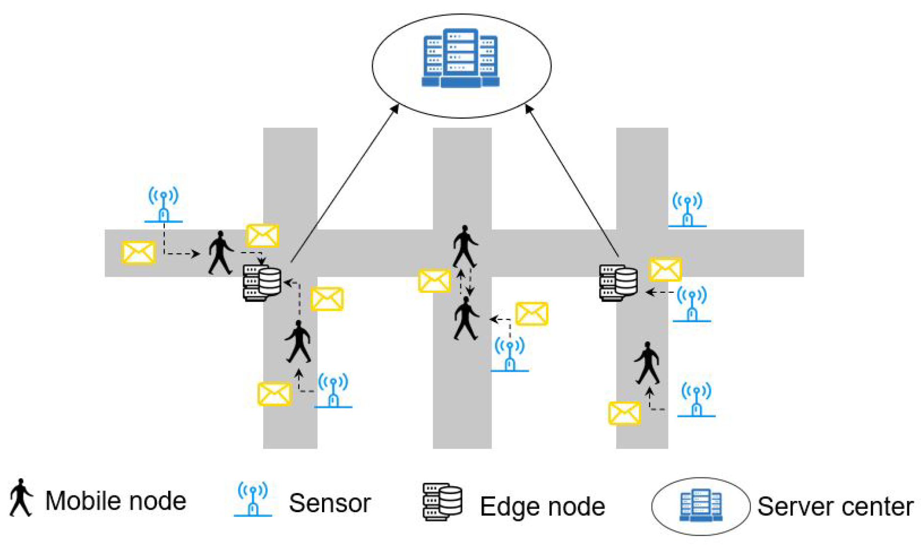
  • Mobile nodes (mobile users): Mobile nodes collect data, such as temperature, images of traffic conditions, and videos of accidents, using the sensors embedded in their smart devices (e.g., camera, microphone, positioning sensor, temperature sensor), and send to edge nodes. They can walk or be in a vehicle to move around the area. When mobile users are in contact with other people or sensors, they can exchange data between them and transmit data to the destination.
  • Sensors: Sensors are deployed in specific locations to collect data, such as air quality, radioactivity, noise levels, and humidity levels. When sensors and destinations (edge nodes) are not directly connected, the sensors must relay packets to mobile users to transfer them to the destinations.
  • Edge nodes: Edge nodes are located in particular locations to gather and preprocess collected data from sensors and mobile users. Then, edge nodes send processed data to the server center.
  • The server center: The server center receives data from edge nodes and uses the received data for urban-sensing applications.
Messages in this network can be of different data types, such as text, images, and video. This model could be used in various applications, such as environmental monitoring [4,5], smart traffic light systems [6], and waste management [31]. For example, in monitoring environmental conditions [4,5], the data from sensors, such as air quality, noise, and radiation sensors, and the data from sensors embedded in smart devices for temperature measurement, are collected and sent to edge nodes. Then, edge nodes preprocess the collected data and send it to the server center.
In this system, edge nodes connect with the server center via an infrastructure network, whereas edge nodes, sensors, and mobile nodes exchange messages with each other using wireless communications such as Bluetooth 5.0. Therefore, this work addresses the problem of how to effectively route data from sensors and mobile nodes to edge nodes. Data collection at edge nodes in this system relies on mobile nodes that move around the city. The selection of nodes for forwarding messages is an important issue. Our work considers network performance in terms of D C , P D L , and P D R . The D C is calculated by dividing the total number of replications by the total number of messages generated. The P D L is the time it takes for messages to be delivered from sources to destinations. The P D R measures the number of messages delivered to their intended destinations divided by the total number of messages.
We assume that the movement histories of a number of mobile nodes are observed, and each node knows its encounter history with other nodes. The information from observed movement history is denoted as M. Let S u N B denote the set of neighboring nodes of node u. The information on the encounter history of nodes in S u N B is denoted E. Node u wants to send a message to edge node v. The objective is to choose relay nodes in S u N B to maximize the P D R and minimize the P D L and the D C , given the information on movement history M and information on encounter history E.

4. The Proposed Routing Algorithm

In this section, the proposed human location prediction model is described in detail. Then, we discuss how to determine packet delivery predictability using the estimated information from the human location prediction model. The social strength of nodes is also calculated using their encounter histories. Finally, a forwarding algorithm is proposed based on those metrics. The routing process of the HLPRP is shown in Figure 2.

4.1. Human Location Prediction (HLP) Model

We propose a human location prediction model based on a RNN and LSTM cells [16] for estimating mobile users’ next positions, using information from their previous movements. In particular, the proposed model takes movement information of mobile users in current and previous time slots as input and outputs estimated locations for the next k time slots.
The information that will be used as input for the prediction model is discussed next. First, to distinguish mobile users, each one is assigned a unique ID. Then, a one-hot vector is used to represent the user ID. Let a u I denote the one-hot vector that indicates the ID of user u. Second, a time slot index is also used as an input feature. The one-hot vector that represents time slot h is denoted a h T . Third, the day of the week is considered. Let a h D be the one-hot vector that indicates the day of the week of time slot h. Fourth, the locations of mobile users are taken into account. The one-hot vector that indicates the location of user u in time slot h is a u , h L . Finally, let t denote the current time slot. From time slot t, the human location prediction model will predict the location of mobile user u in the next time slot, q (e.g., with k = 4 , q could be time slot t + 1 , time slot t + 2 , time slot t + 3 , or time slot t + 4 ). To determine time slot q, a one-hot vector is used. Let a P T denote the time slot in which we want to predict the location of user u. a P T is considered an input feature as well. One-hot encoding is used for all input features because those features are nominal and not ordinal. The input will be information from time slot ( t m + 1 ) to current time slot t. Let us define x u , h as the input vector of user u in time slot h, specifically, x u , h = { a P T , a u I , a h D , a h T , a u , h L } .
This model is based on a RNN with LSTM cells. After the last hidden state of the LSTM cell, a fully connected layer with ReLU activation and a fully connected layer with a softmax activation function is used for the output layer. Let y ^ u , q denote the output vector that shows the probability that mobile user u will visit locations in time slot q (e.g., q = t + 1 ). For example, y ^ u , q = [ 0.1 , 0.05 , 0.01 , , 0.3 ] means that in time slot q, the probability of visiting the first location is 0.1; the probability of visiting the second location is 0.05 , and so on. The notations used in the human location prediction model are shown in Table 1.

4.2. Packet Delivery Predictability

In the network model, edge nodes are deployed at certain locations. Suppose that edge node v is located at a certain location in the area. The probability that a mobile user visits edge node v from time slot t + 1 to time slot t + k is obtained by using the human location prediction model. Let p ( u , v ) t + j denote the probability that mobile user u visits edge node v at time slot t + j . Based on the visit probability, packet delivery predictability (the possibility that a node will deliver a packet to its destination) can be calculated. Let D P ( u , v ) t denote the packet delivery predictability of mobile user u to edge node v in time slot t. D P ( u , v ) t is calculated as follows:
D P ( u , v ) t = j = 1 k ( p ( u , v ) t + j ) α × j
where a tunable parameter, α ( 0 , 1 ) , is used to adjust the effect of probabilities based on time. Specifically, with ( α × j ) , the probability for a time slot in the distant future has less effect on the value of D P ( u , v ) t than the probability for a time slot in the near future (e.g., p ( u , v ) t + 2 affects D P ( u , v ) t less than p ( u , v ) t + 1 ). In other words, a node with a high visit probability in the near future has higher packet delivery predictability than a node with a high visit probability in the distant future. A high D P ( u , v ) t value indicates that a message can be delivered from mobile user u to edge node v with high probability and low latency. Therefore, a relay node with high packet delivery predictability is preferable.

4.3. Social Strength

Social strength is used to represent the social relationships between nodes in the network. To measure the social strength between nodes, connection characteristics such as encounter frequency [32] and contact duration [33,34] can be used. In this work, social strength is determined based on contact duration between nodes. During the observation time, nodes that have been in touch for a longer period have a higher social strength. Contacts between nodes are assumed to be collected over a time period, T C . Let η represent the number of contacts between node u and node v. The duration of the i t h contact between node u and node v is defined as C T u , v i . Let s ( u , v ) denote the social strength between node u and node v. Then, s ( u , v ) is calculated as:
s ( u , v ) = i = 1 η C T u , v i T C
From Equation (2), we see that the social strength of two nodes is the total contact duration between them over the time period of collecting contacts between nodes. A high value for s ( u , v ) implies that they have a close relationship and usually encounter each other.

4.4. Forwarding Algorithm

The proposed forwarding algorithm, based on packet delivery predictability and social strength, is presented in Algorithm 1. The notations used in the algorithm are defined in Table 2.
Algorithm 1 The forwarding algorithm
1:
Node u has packet p to send to edge node v
Input: S u N B , D P ( u , v ) t , s ( u , v ) , α , D u , c u p
2:
for each i S u N B do
3:
    if  c u p > 1  then
4:
        Node u selects node i as a relay node and forwards a copy of packet p to i
5:
         c i p = min ( max ( c u p × D i D i + D u + ϵ , 1 ) , c u p 1 )
6:
         c u p = c u p c i p
7:
    else if  c u p = 1  then
8:
        if  D P ( i , v ) t > D P ( u , v ) t  then
9:
           Node i is chosen as a relay node for packet p
10:
        else if  D P ( i , v ) t = D P ( u , v ) t and s ( i , v ) > s ( u , v )  then
11:
           Node i is chosen as a relay node for packet p
12:
        end if
13:
        if Node i is chosen as a relay node for packet p then
14:
           Node u forwards packet p to node i and deletes packet p from buffer
15:
            c i p = 1
16:
        end if
17:
    end if
18:
end for
Assume that node u wants to send packet p to edge node v. First, the neighboring nodes of node u are checked. If the destination is listed in the neighboring nodes, the packet is delivered to the destination. Otherwise, the forwarding process is executed following Algorithm 1.
In the forwarding algorithm, a forwarding token for packets is used to limit the number of copies of packets in the network similarly in [11,15]. Specifically, when a node generates a packet, it also assigns a forwarding token to the packet. The forwarding token’s initial value is C. Let c u p represent the forwarding token for packet p of node u. The forwarding algorithm is processed in two phases based on the value of c u p . In phase 1, i.e., when c u p > 1 , packets are quickly spread in the network, and degree centrality is used to update the forwarding token’s value. In phase 2, when c u p = 1 , relay nodes are selected based on packet delivery predictability and social strength.
Specifically, in phase 1 when c u p > 1 , node u selects node i in S u N B as a relay node and forwards a copy of packet p to node i without consideration of any other condition in line 4. Based on the social strength between nodes, a social graph is constructed. In the social graph, vertices are nodes, and there is a link between two nodes if their social strength is greater than zero. The degree centrality of a node is defined as the number of links between itself and other nodes in the social graph. To update the forwarding token’s value, degree centrality is used. Let D u and D i represent the degree centrality of node u and the degree centrality of node i, respectively. The forwarding token’s value assigned to the copy of packet p at node i is denoted as c i p , which is calculated as follows:
c i p = min ( max ( c u p × D i D i + D u + ϵ , 1 ) , c u p 1 )
where a very small value, ϵ , is added to avoid the denominator being zero. According to Equation (3), c i p is limited to values between [ 1 , c u p 1 ] , and a node with a larger value for the degree centrality will be assigned a greater forwarding token’s value. In the real context, a node with a high degree of centrality has a greater likelihood of connecting with other nodes. If it has a large value for the forwarding token, copies of the packet will quickly spread throughout the network. That supports minimizing P D L and enhances the possibility of delivering the packet to its destination. In Algorithm 1, c i p is calculated in line 5, and c u p is updated in line 6 (i.e., c u p = c u p c i p ).
In phase 2, when c u p = 1 , the packet delivery predictabilities are compared in line 8. If node i has a greater packet delivery predictability with edge node v than node u (i.e., D P ( i , v ) t > D P ( u , v ) t ), node i is chosen as a relay node for packet p in line 9. Otherwise, if D P ( i , v ) t = D P ( u , v ) t , social strengths are compared in line 10. Specifically, if D P ( i , v ) t = D P ( u , v ) t and s ( i , v ) > s ( u , v ) , node i is selected as a relay node for packet p in line 11. Finally, if node i is chosen as the relay node for packet p, node u will forward packet p to node i and delete packet p from its buffer (line 14). The forwarding token’s value for packet p at node i, c i p , is set to 1 (line 15).

5. Evaluation Results

In this section, first, a Wi-Fi scan dataset is presented. Then, the simulation setup is discussed. The results of the proposed HLP model are presented and compared with the results of the Markov model [35]. The performance of the proposed routing protocol is evaluated in terms of D L , P D L , and D C . The proposed routing is compared with the spray-and-wait routing protocol [11], epidemic routing [9], CORP [14], PRoPHET [13], and BUBBLE Rap [26]. The opportunistic networking environment (ONE) simulation tool [36] is used for simulation.

5.1. Dataset

The UB/phonelab-wifi logs were gathered over a five-month period from the smartphones of 284 faculty members, staff, and students at the University at Buffalo [17]. We specifically use the sub-dataset named WifiScanResult, which includes the Wi-Fi scan records of 274 anonymous mobile users and about 1.1 million access point (AP) scans. When a phone scans for and finds a nearby AP, it records information, such as the timestamp, device ID, basic service set identifier (BSSID), and signal strength. Most people carry their phones, and indoor Wi-Fi APs often have short transmission ranges of tens of meters. Thus, the human movement could be represented as a sequence of scanned APs identifiable by their BSSIDs [37]. A smartphone can scan and detect several APs at one time. The scanned AP with the highest signal strength is chosen to reflect mobile users’ positions.
We focus on data collected over 90 days from 1 January to 31 March 2015. During this period, the most Wi-Fi activities for all selected mobile users, as well as their interactions, can be observed. Then, the 50 most active users and 1243 of the most visited APs are chosen as input data for building our proposed human location prediction model. An extra dummy AP is added for a time slot in which there are no scanned APs. The proposed model estimates mobile users’ locations from 9 a.m. to 6 p.m. (the most active period of the day). Therefore, to train the model, human movement from 8 a.m. to 6 p.m. is extracted. Specifically, the time period from 8 a.m. to 6 p.m. is divided into 41 time slots of 15 minutes (including the last time slot from 6 p.m. to 6:15 p.m.), and then, each data sample’s timestamp is mapped to one of the predefined 41 time slots. During a time slot, the latest position of the user is considered the user’s position for that whole time slot.
Because the UB dataset is sparse, there are a lot of dummy labels. To prevent the model from predicting the dummy location as the next location, all training and validation samples containing dummy labels are removed. Note that only dummy locations from the label are removed, allowing for the possibility of dummy locations in input samples. Following the data extraction procedures mentioned above, we derive a new dataset from which to build the proposed human location prediction model.

5.2. Simulation Setup

The data for 13 February 2015, is used to simulate the proposed routing protocol. The remaing 89 days are used to train and test the human location prediction model. The simulation’s duration is set to nine hours (i.e., from 9 a.m. to 6 p.m.). The number of edge nodes and the number of sensors are set to 5 and 50, respectively. These nodes are randomly placed at locations of frequently scanned APs. Specifically, from 20 access points (APs) that have the highest number of scanned times by mobile users, five APs are randomly selected as locations to deploy five edge nodes. From 150 APs that have the highest number of scanned times by mobile users, 50 APs are randomly selected as locations to deploy sensors. Using this method, the edge nodes and the sensor nodes are deployed to locations that are frequently visited by mobile nodes. In other words, they are deployed at locations with a high density of mobile users. Note that in order to reflect a more realistic scenario in this work, a scenario in which some of the users have predictable mobility and the rest have unpredictable mobility is considered. Therefore, the 50 most active users were selected from the UB dataset and were considered users with predictable mobility. The human location prediction model is trained and tested using the movement history of those people. Thus, their future locations can be predicted using the model. Moreover, we also select 100 additional mobile users from the UB dataset and assume that they have no movement history. The locations of those nodes are unpredictable. Therefore, their packet delivery predictability is set to zero. However, in the network model, it is also supposed that each node knows its encounter history with other nodes. Therefore, the social strength of those 100 mobile users can still be determined. Finally, the total number of mobile nodes is 150 (i.e., 50 mobile users with movement history and 100 mobile users without movement history).
The media access control (MAC) layer of Bluetooth 5.0 with a transmission rate of 2 Mbps is used. Bluetooth 5.0 is designed for very low power operation. That reduces power usage and extends battery life for nodes. The UB dataset provides the Wi-Fi scan records of mobile devices. Indoor Wi-Fi APs often have short transmission ranges of tens of meters. There is no physical location information for APs and mobile users in the UB dataset. The real distance between nodes cannot be obtained. Therefore, we assume that a mobile user communicates with another mobile user if they scan and detect at least one common AP. In addition, a mobile user communicates with a sensor or an edge node if the user scans and detects the AP where the sensor or the edge node is placed. Packets are generated with a size of 500 bytes (e.g., the size of sensing data or a text message), and the generation interval is randomly set at between 25 s and 30 s. We consider the network model that allows messages with a long expiration time. Therefore, the time to live (TTL) for packets was set to four hours. Each node has a buffer that can store 150 packets. The first-in-first-out (FIFO) buffer is used. The initial value of forwarding token C is set to 64. In addition, the proposed protocol is also compared with other routing protocols. Common parameters, such as the number of nodes and the MAC layer are the same in all routing protocols. The forwarding token under spray-and-wait is set at the same value in the HLPRP. Under PRoPHET, first, the initialization constant of delivery predictability, P i n i t , was set to 0.75. Then, the scaling constant, β , and aging constant, γ , were set to 0.25 and 0.98, respectively. For CORP, the threshold of minimum probability and the threshold of maximum probability are set to 0.45 and 0.88, respectively. The K value for K-clique in BUBBLE Rap is set to three. Table 3 shows the details for the simulation parameters.

5.3. The Results of the Proposed Human Location Prediction Model
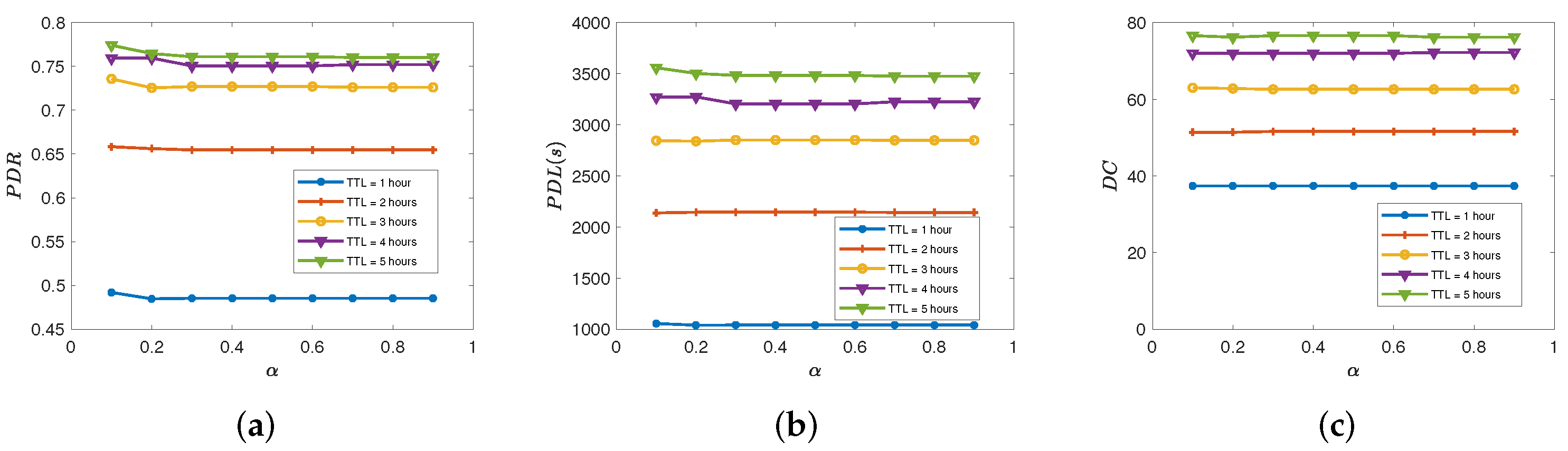
Table 4 presents the top-1 accuracy of the prediction models when predicting users’ locations in various future time slots (i.e., t + 1 , t + 2 , t + 3 , t + 4 ). In general, our proposed model obtains higher accuracy than the Markov model. Top-1 accuracy achieves the highest value when predicting the users’ locations in the next time slot, t + 1 , and then decreases slightly at time slots in the further future. This indicates that the movement history of mobile users has a greater impact on their locations in the near future than on their locations in the further future. The average accuracy from the proposed HLP model is 0.5831 . This indicates that the proposed model can work well. Using the predicted information, the values of packet delivery predictability are obtained for the routing algorithm.

5.4. Effects of α on the Performance of the Proposed Routing Protocol

In this subsection, the effects of α on the performance of the HLPRP are discussed. Recall that when calculating packet delivery predictability, we can adjust the effect on packet delivery predictability of the predicted information for the near future and the distant future by using tunable parameter α . Figure 3 shows the network performance for various values of α and T T L . The P D R is shown in Figure 3a. In general, the P D R is higher with a longer T T L . For the same value of T T L , the P D R does not change much. For example, with T T L = 4 h, it reduces slightly when α increases from 0.1 to 0.3, and then it slightly increases from 0.7506 to 0.7521 when α increases from 0.6 to 0.7. Figure 3b displays the P D L . The P D L increases when the T T L increases. For low values of α , latency is high. Then, it decreases when α increases. For example, with the T T L = 4 h, the P D L is 3269 s when α = 0.1 and 3225 s when α = 0.7 . The D C is presented in Figure 3c. The D C is larger with a longer T T L . The value of α does not affect the D C much. It is similar for the various values of α . For example, the D C is 37.4 when the T T L = 1 h for all different values of α .
From the obtained results in Figure 3, the value of α was set to 0.7 in the proposed routing protocol.

5.5. Effects of Packet TTL on Routing Protocol Performance

Figure 4 shows the network performance for various TTL values. First, the results for the P D R are presented in Figure 4a. Overall, the figure shows that increasing the lifetime of packets increases the P D R to a certain point, and then it stabilizes under the HLPRP, CORP, BUBBLE Rap, and spray-and-wait routing protocols but decreases under epidemic routing and PRoPHET. CORP tries to forward the packet to the community of the destination. In a sparse network, nodes belonging to two distinct communities rarely communicate with one another. Hence, there are very few nodes that can be selected as relay nodes. As a result, CORP obtained the lowest values for the P D R . In BUBBLE Rap, by using global rank (i.e., betweenness centrality), a message has a better chance of being forwarded to the destination’s community. Therefore, the P D R from BUBBLE Rap is higher than CORP. The number of packet copies was not limited in PRoPHET and epidemic routing. Thus, the buffer quickly filled when the TTL increased, and a large number of packets were dropped, resulting in a low value for the P D R . For example, the P D R of PRoPHET reduces from 0.6874 to 0.5363 when the T T L increases from 3 h to 6 h. In the spray-and-wait routing protocol, buffer overflow was reduced by the limited number of replications. Therefore, the P D R of the spray-and-wait is greater than that of PRoPHET and epidemic routing. By limiting the number of copies of packets, the HLPRP can also reduce buffer overflow. Moreover, relay selection is based on packet delivery predictability and social relationships. Optimal relay nodes can be found, and hence, the P D R under the HLPRP is improved and is higher than those of the other protocols. For example, when the TTL is 6 h, the P D R of the HLPRP, spray-and-wait routing, PRoPHET, BUBBLE Rap, CORP, and epidemic routing are 0.7645, 0.7450, 0.5363, 0.5335, 0.4371, and 0.4074, respectively.
Latency from various values for the packet TTL is illustrated in Figure 4b. In general, a larger value for TTL means packets can be stored in the buffer for longer, which leads to an increased P D L , as shown in the figure. Under CORP and PRoPHET, a packet is slowly spread due to the absence of a rapid packet-spreading mechanism. This results in a significant increase in the P D L . Based on the flooding strategy, the P D L under epidemic routing is low. In the HLPRP, packets are quickly spread during phase 1, and nodes with a higher probability of meeting the destination in a short period of time are preferred as relay nodes during phase 2. Therefore, the HLPRP also achieves a short delay, comparable to that of epidemic routing, and shorter than the other protocols. For example, when the TTL is 5 h, the P D L of the HLPRP and epidemic routing are 3476 s and 3470 s, whereas spray-and-wait routing, PRoPHET, BUBBLE Rap, and CORP are 3626 s, 3862 s, 3516 s, and 3667 s, respectively.
Figure 4c shows the results for the D C . Under PRoPHET and epidemic routing, the number of packet copies is not limited. As a result, the D C is extremely high. When the TTL increases, the buffer overflows, and a large number of packets are dropped. That leads to a quickly increasing D C under those protocols. In CORP, by finding the node in the destination’s community before finding the destination, the D C is reduced. BUBBLE Rap uses betweenness centrality to select relay nodes until meeting nodes in the destination’s community. Therefore, the number of transmissions of messages is higher than in CORP. As a result, the D C under BUBBLE Rap is higher than that under CORP. By limiting the number of replications with the spray-and-wait routing protocol, a low value of the D C can be obtained. Under the HLPRP, the number of copies of a packet in the network is also limited. The D C from the HLPRP is also reduced and is lower than that from PRoPHET, CORP, and epidemic routing. For example, when the packet TTL is 2 h, the D C from the HLPRP, the spray-and-wait routing protocol, CORP, and BUBBLE Rap are 51.6, 22.4, 96.6, and 406.8, respectively, whereas PRoPHET and epidemic routing reach 709.6 and 1636.2, respectively. The HLPRP’s D C is greater than the spray-and-wait routing protocol’s because when the forwarding token value is equal to 1, the HLPRP continues to forward the packet if a better relay node is found, whereas the spray-and-wait routing protocol waits until it reaches the destination.

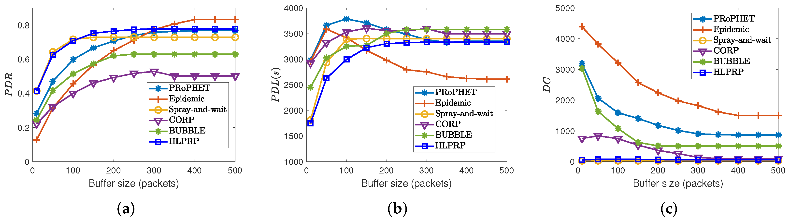
5.6. Effects of Buffer Size on Routing Protocol Performance

Figure 5 shows the network performance for various buffer sizes. First, the P D R is presented in Figure 5a. A larger buffer means that it can forward and store more packets. Thus, as shown in Figure 5a, the P D R increases as the buffer size increases. By using the predicted information and the social strength between nodes, our routing protocol can achieve a greater P D R than others when the buffer size is between 10 and 250 packets. When the buffer size is very large, buffer overflow is reduced in the flooding strategy. Specifically, epidemic routing obtains high values for the P D R when the buffer capacity is larger than 300 packets. However, the flooding strategy also consumes a significant amount of network resources.
P D L results are in Figure 5b. A small buffer (e.g., 10 packets) will quickly overflow. As a result, it removes packets with long delays to make room for the new ones coming. Therefore, the buffer contains only packets with short delays. This results in low P D L . When the buffer size increases, it can contain more packets with longer delays, which increases latency. The shortest latency is obtained by the HLPRP when the buffer capacity is between 10 and 100 packets. In epidemic routing, a large buffer can store more packets. Packets are quickly sent to their destinations without being dropped. Hence, epidemic routing with a large buffer (e.g., 300 packets) has a short P D L .
Figure 5c shows the results for the D C . When the buffer is small, numerous packets are lost and retransmitted due to buffer overflow under epidemic routing and PRoPHET. That creates a huge D C . The D C from the HLPRP is lower than that from PRoPHET, CORP, BUBBLE Rap, and epidemic routing.

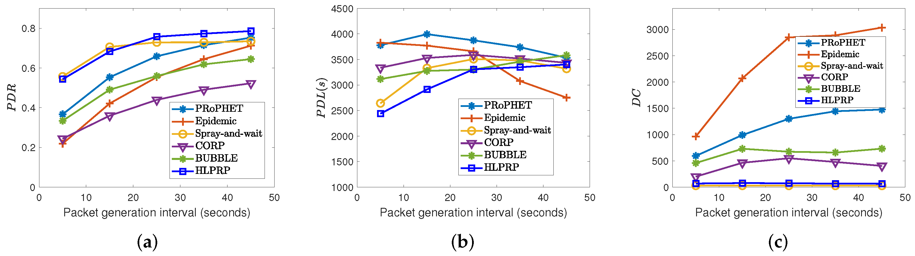
5.7. Effects of the Packet Generation Interval on Routing Protocol Performance

In Figure 6, network performance for various packet generation intervals is shown. The results for the P D R are illustrated in Figure 6a. In general, increasing the packet generation interval will reduce network traffic. Thus, the P D R tends to increase as the packet generation interval increases. By rapidly spreading packets and selecting optimal relay nodes based on the predicted information and social relationships, the HLPRP achieves a better P D R than the others when the packet generation interval is between 25 s and 45 s.
Figure 6b shows the results of the P D L . The latency from the HLPRP is lower than from other routing protocols when the packet generation interval varies between 5 s and 25 s. When network traffic is light (i.e., the packet generation interval is between 35 s and 45 s), using the flooding strategy, epidemic routing obtains the shorter delivery latency. However, the D C from epidemic routing is huge, as shown in Figure 6c. Figure 6c also indicates that the HLPRP has a lower D C than CORP, PRoPHET, BUBBLE Rap, and epidemic routing.

6. Conclusions

In this paper, we proposed a novel routing protocol for mobile crowdsensing-based urban sensor networks based on human location prediction. Specifically, a RNN-based model using LSTM cells was built for estimating the locations of mobile nodes. Useful information, such as nodes’ identities, time slots in the day, the day of the week, and node location is extracted from the dataset. That information is used to train and test the prediction model. Packet delivery predictability is proposed by using the probabilities obtained from the prediction model. From the encounter histories of the nodes, social strength between them is also determined and considered in the proposed routing algorithm. Specifically, the HLPRP is processed in two phases. In the first phase, the degree centrality is used to determine the forwarding token value of relay nodes. That helps to quickly spread the packets throughout the network. In the second phase, packet delivery predictability and social strength are used to select optimal relay nodes. The network performance under the HLPRP was evaluated by comparing it with that of other routing protocols in terms of P D R , P D L , and D C . The obtained results showed that the HLPRP can outperform the other routing protocols. In future work, the effect of social aspects (e.g., information about nodes that have strong social relationships) will be considered to predict the human location. Additionally, we plan to study a routing protocol based on reinforcement learning in which the agent’s action is to select relay nodes based on current state information such as social strength, packet delivery predictability, and spatial information.

Author Contributions

Conceptualization, D.V.A.D. and S.Y.; data curation, D.V.A.D. and S.Y.; formal analysis, D.V.A.D. and S.Y.; funding acquisition, S.Y.; investigation, D.V.A.D. and S.Y.; methodology, D.V.A.D. and S.Y.; project administration, S.Y.; supervision, S.Y.; validation, D.V.A.D.; writing—original draft, D.V.A.D. and S.Y.; writing—review and editing, D.V.A.D. and S.Y. All authors have read and agreed to the published version of the manuscript.

Funding

This work was supported by the 2021 Research Fund of University of Ulsan.

Institutional Review Board Statement

Not applicable.

Informed Consent Statement

Not applicable.

Conflicts of Interest

The authors declare no conflict of interest.

References

  1. Capponi, A.; Fiandrino, C.; Kantarci, B.; Foschini, L.; Kliazovich, D.; Bouvry, P. A Survey on Mobile Crowdsensing Systems: Challenges, Solutions, and Opportunities. IEEE Commun. Surv. Tutor. 2019, 21, 2419–2465. [Google Scholar] [CrossRef] [Green Version]
  2. Boubiche, D.E.; Imran, M.; Maqsood, A.; Shoaib, M. Mobile crowd sensing—Taxonomy, applications, challenges, and solutions. Comput. Hum. Behav. 2019, 101, 352–370. [Google Scholar] [CrossRef]
  3. Liu, Y.; Kong, L.; Chen, G. Data-Oriented Mobile Crowdsensing: A Comprehensive Survey. IEEE Commun. Surv. Tutor. 2019, 21, 2849–2885. [Google Scholar] [CrossRef]
  4. Wu, D.; Xiao, T.; Liao, X.; Luo, J.; Wu, C.; Zhang, S.; Li, Y.; Guo, Y. When Sharing Economy Meets IoT: Towards Fine-Grained Urban Air Quality Monitoring through Mobile Crowdsensing on Bike-Share System. Proc. ACM Interact. Mob. Wearable Ubiquitous Technol. 2020, 4, 1–26. [Google Scholar] [CrossRef]
  5. Jiang, F.; Sun, Y.; Sha, J. Crowd Sensing Urban Healthy Street Monitoring Based on Mobile Positioning System. Mob. Inf. Syst. 2021, 2021, 9394063. [Google Scholar] [CrossRef]
  6. Ali, A.; Qureshi, M.A.; Shiraz, M.; Shamim, A. Mobile crowd sensing based dynamic traffic efficiency framework for urban traffic congestion control. Sustain. Comput. Inform. Syst. 2021, 32, 100608. [Google Scholar] [CrossRef]
  7. Jiang, Z.; Zhu, H.; Zhou, B.; Lu, C.; Sun, M.; Ma, X.; Fan, X.; Wang, C.; Chen, L. CrowdPatrol: A Mobile Crowdsensing Framework for Traffic Violation Hotspot Patrolling. IEEE Trans. Mob. Comput. 2021. [Google Scholar] [CrossRef]
  8. Kutsarova, V.; Matskin, M. Combining Mobile Crowdsensing and Wearable Devices for Managing Alarming Situations. In Proceedings of the 2021 IEEE 45th Annual Computers, Software, and Applications Conference (COMPSAC), Madrid, Spain, 12–16 July 2021; pp. 538–543. [Google Scholar]
  9. Vahdat, A.; Becker, D. Epidemic Routing for Partially-Connected Ad Hoc Networks; Technical Report CS-2000-06; Duke University: Durham, NC, USA, 2000. [Google Scholar]
  10. Garg, P.; Kumar, H.; Johari, R.; Gupta, P.; Bhatia, R. Enhanced Epidemic Routing Protocol in Delay Tolerant Networks. In Proceedings of the 2018 5th International Conference on Signal Processing and Integrated Networks (SPIN), Noida, India, 22–23 February 2018; pp. 396–401. [Google Scholar]
  11. Spyropoulos, T.; Psounis, K.; Raghavendra, C.S. Spray and Wait: An Efficient Routing Scheme for Intermittently Connected Mobile Networks. In Proceedings of the 2005 ACM SIGCOMM Workshop on Delay-tolerant Networking, Philadelphia, PA, USA, 26 August 2005; pp. 252–259. [Google Scholar]
  12. Duong, D.V.A.; Yoon, S. An Efficient Probabilistic Routing Algorithm Based on Limiting The Number of Replications. In Proceedings of the 2019 International Conference on Information and Communication Technology Convergence, Jeju Island, Korea, 16–18 October 2019; pp. 562–564. [Google Scholar] [CrossRef]
  13. Lindgren, A.; Doria, A.; Schelén, O. Probabilistic Routing in Intermittently Connected Networks. In Service Assurance with Partial and Intermittent Resources; Springer: Berlin/Heidelberg, Germany, 2004; pp. 239–254. [Google Scholar]
  14. Haoran, S.; Muqing, W.; Yanan, C. A Community-Based Opportunistic Routing Protocol in Delay Tolerant Networks. In Proceedings of the 2018 IEEE 4th International Conference on Computer and Communications (ICCC), Chengdu, China, 7–10 December 2018; pp. 296–300. [Google Scholar]
  15. Duong, D.V.A.; Kim, D.Y.; Yoon, S. TSIRP: A Temporal Social Interactions-Based Routing Protocol in Opportunistic Mobile Social Networks. IEEE Access 2021, 9, 72712–72729. [Google Scholar] [CrossRef]
  16. Sherstinsky, A. Fundamentals of Recurrent Neural Network (RNN) and Long Short-Term Memory (LSTM) network. Phys. D Nonlinear Phenom. 2020, 404, 132306. [Google Scholar] [CrossRef] [Green Version]
  17. Shi, J.; Qiao, C.; Koutsonikolas, D.; Challen, G. CRAWDAD Dataset Buffalo/Phonelab-Wifi (v. 2016-03-09). 2016. Available online: https://crawdad.org/buffalo/phonelab-wifi/20160309 (accessed on 24 August 2021).
  18. Ahmed, M.; Goyal, S.; Singh, S.; Gupta, J. An improved Spray and Wait routing protocol for Delay Tolerant Network. In Proceedings of the 2019 2nd IEEE Middle East and North Africa COMMunications Conference (MENACOMM), Manama, Bahrain, 19–21 November 2019; pp. 1–6. [Google Scholar]
  19. Abdajbar, A.N.; Mohamed, K.S.; Alias, M.Y. Link Budget Based Optimised Link State Routing Protocol in Flying Ad-hoc Networks. In Proceedings of the 2019 IEEE Conference on Sustainable Utilization and Development in Engineering and Technologies (CSUDET), Penang, Malaysia, 7–9 November 2019; pp. 261–264. [Google Scholar]
  20. Arnous, R.; El-kenawy, E.S.M.T.; Saber, M. A Proposed Routing Protocol for Mobile Ad Hoc Networks. Int. J. Comput. Appl. 2019, 975, 8887. [Google Scholar] [CrossRef]
  21. Wang, G.; Wang, J.; Wang, B. An adaptive spray and wait routing algorithm based on capability of node in DTN. J. Inf. Comput. Sci. 2014, 11, 1975–1982. [Google Scholar] [CrossRef]
  22. Lenando, H.; Alrfaay, M. Epsoc: Social-based epidemic-based routing protocol in opportunistic mobile social network. Mob. Inf. Syst. 2018, 2018, 6462826. [Google Scholar] [CrossRef] [Green Version]
  23. Raghav, N.; Kumar, A. Routing Strategy based on Centrality in Opportunistic Networks. In Proceedings of the 2019 6th International Conference on Computing for Sustainable Global Development (INDIACom), New Delhi, India, 13–15 March 2019; pp. 922–926. [Google Scholar]
  24. Yim, J.; Ahn, H.; Ko, Y.B. The betweenness centrality based geographic routing protocol for unmanned ground systems. In Proceedings of the 10th International Conference on Ubiquitous Information Management and Communication, Danang, Vietnam, 4–6 January 2016; pp. 1–4. [Google Scholar]
  25. Bulut, E.; Szymanski, B.K. Exploiting Friendship Relations for Efficient Routing in Mobile Social Networks. IEEE Trans. Parallel Distrib. Syst. 2012, 23, 2254–2265. [Google Scholar] [CrossRef]
  26. Hui, P.; Crowcroft, J.; Yoneki, E. BUBBLE Rap: Social-Based Forwarding in Delay-Tolerant Networks. IEEE Trans. Mob. Comput. 2011, 10, 1576–1589. [Google Scholar] [CrossRef] [Green Version]
  27. Wang, G.; Zheng, L.; Yan, L.; Zhang, H. Probabilistic routing algorithm based on transmission capability of nodes in DTN. In Proceedings of the 2017 11th IEEE International Conference on Anti-counterfeiting, Security, and Identification, Xiamen, China, 27–29 October 2017; pp. 146–149. [Google Scholar]
  28. Vanitha, N. Binary Spray and wait routing Protocol with controlled replication for DTN based Multi-Layer UAV Ad-hoc network Assisting VANET. Turkish J. Comput. Math. Educ. (TURCOMAT) 2021, 12, 276–2782. [Google Scholar]
  29. Kuronuma, Y.; Suzuki, H.; Koyama, A. An Adaptive DTN Routing Protocol Considering Replication State. In Proceedings of the 2017 31st International Conference on Advanced Information Networking and Applications Workshops, Taipei, Taiwan, 27–29 March 2017; pp. 421–426. [Google Scholar]
  30. Kaur, H.; Kaur, H. An enhanced spray-copy-wait DTN routing using optimized delivery predictability. In Computer Communication, Networking and Internet Security; Springer: Berlin, Germany, 2017; pp. 603–610. [Google Scholar]
  31. Bonino, D.; Alizo, M.T.D.; Pastrone, C.; Spirito, M. WasteApp: Smarter waste recycling for smart citizens. In Proceedings of the 2016 International Multidisciplinary Conference on Computer and Energy Science (SpliTech), Split, Croatia, 13–15 July 2016; pp. 1–6. [Google Scholar]
  32. Basta, N.; ElNahas, A.; Grossmann, H.P.; Abdennadher, S. A Framework for Social Tie Strength Inference in Vehicular Social Networks. In Proceedings of the 2019 Wireless Days (WD), Manchester, UK, 24–26 April 2019; pp. 1–8. [Google Scholar]
  33. Li, C.; Jiang, F.; Wang, X.; Shen, B. Optimal relay selection based on social threshold for D2D communications underlay cellular networks. In Proceedings of the 2016 8th International Conference on Wireless Communications Signal Processing (WCSP), Yangzhou, China, 13–15 October 2016; pp. 1–6. [Google Scholar]
  34. Moradi, S.; Mohasefi, J.B.; Mahdipour, E. MSN-CDF: New community detection framework to improve routing in mobile social networks. Int. J. Commun. Syst. 2021, 34, e4989. [Google Scholar] [CrossRef]
  35. Gagniuc, P.A. Markov Chains: From Theory to Implementation and Experimentation; John Wiley & Sons: Hoboken, NJ, USA, 2017. [Google Scholar]
  36. Keränen, A.; Ott, J.; Kärkkäinen, T. The ONE Simulator for DTN Protocol Evaluation. In Proceedings of the SIMUTools ’09: Proceedings of the 2nd International Conference on Simulation Tools and Techniques, Rome, Italy, 2–6 March 2009. [Google Scholar]
  37. Shi, J.; Meng, L.; Striegel, A.; Qiao, C.; Koutsonikolas, D.; Challen, G. A walk on the client side: Monitoring enterprise Wifi networks using smartphone channel scans. In Proceedings of the IEEE INFOCOM 2016—The 35th Annual IEEE International Conference on Computer Communications, San Francisco, CA, USA, 10–14 April 2016; pp. 1–9. [Google Scholar]
Figure 1. The network model.
Applsci 12 03898 g001
Figure 2. The HLPRP routing process.
Applsci 12 03898 g002
Figure 3. The network performance for various values of α . (a) P D R . (b) P D L . (c) D C .
Applsci 12 03898 g003
Figure 4. The network performance for various values of packet time to live. (a) P D R . (b) P D L . (c) D C .
Applsci 12 03898 g004
Figure 5. The network performance for various buffer sizes. (a) P D R . (b) P D L . (c) D C .
Applsci 12 03898 g005
Figure 6. The network performance for various values of the packet generation interval. (a) P D R . (b) P D L . (c) D C .
Applsci 12 03898 g006
Table 1. Notations used in the human location prediction model.
NotationMeaning
x u , h Input vector of user u in time slot h
a P T One-hot vector: the next time slot for prediction of the user’s location
a u I One-hot vector: the ID of mobile user u
a h D One-hot vector: the day of the week of time slot h
a h T One-hot vector: presents time slot h
a u , h L One-hot vector: the location of user u in time slot h
y ^ u , q Output vector
Table 2. Notations used in the proposed forwarding algorithm.
NotationMeaning
D P ( u , v ) t The packet delivery predictability between node u and node v in time slot t
s ( u , v ) The social strength between node u and node v
D u The degree centrality of node u
c u p The forwarding token of node u for packet p
S u N B The set of neighboring nodes of node u
Table 3. Simulation parameters.
ParameterValue
Simulation duration9 h
Number of edge nodes5
Number of sensors50
Number of mobile users with movement history50
Number of mobile users without movement history100
Transmission rate2 Mbps
Packet generation interval25–30 s
Buffer size150 packets
Packet TTL4 h
Packet size500 bytes
Initial value of forwarding token (C)64
Table 4. Top-1 accuracy from the prediction models.
Prediction ModelTime
Slot
t + 1
Time
Slot
t + 2
Time
Slot
t + 3
Time
Slot
t + 4
Average
The proposed HLP model0.61020.59070.57350.55550.5831
The Markov model0.60300.56360.53380.50970.5535
Publisher’s Note: MDPI stays neutral with regard to jurisdictional claims in published maps and institutional affiliations.

