Structural Damage Prediction of a Reinforced Concrete Frame under Single and Multiple Seismic Events Using Machine Learning Algorithms

Abstract

Advanced machine learning algorithms have the potential to be successfully applied to many areas of system modelling. In the present study, the capability of ten machine learning algorithms to predict the structural damage of an 8-storey reinforced concrete frame building subjected to single and successive ground motions is examined. From this point of view, the initial damage state of the structural system, as well as 16 well-known ground motion intensity measures, are adopted as the features of the machine-learning algorithms that aim to predict the structural damage after each seismic event. The structural analyses are performed considering both real and artificial ground motion sequences, while the structural damage is expressed in terms of two overall damage indices. The comparative study results in the most efficient damage index, as well as the most promising machine learning algorithm in predicting the structural response of a reinforced concrete building under single or multiple seismic events. Finally, the configured methodology is deployed in a user-friendly web application.

1. Introduction

During earthquake events, it is common to observe aftershocks following a mainshock. Moderate-to-strong aftershocks may lead to additional structural damage and even the collapse of buildings that sustained damage from the mainshock. Thus, the seismic performance of structural systems subjected to successive ground motions has received increasing attention in recent years. The recent disaster that occurred on March 2021 in the Tyrnavos–Elassona region, Thessaly of Greece due to a pair of compatible magnitude (Mw = 6.3, Mw = 6.1) [1] shallow earthquakes with more than 1800 damaged or non-serviceable buildings demonstrated the necessity of predicting the damage potential caused by mainshock–aftershock sequences in order to assess the seismic risk. It should be noted that the final, accumulated damage includes the initial damage caused by the major earthquake and the incremental damage caused by the following seismic sequence. The effect of successive seismic events on the structural performance has been thoroughly examined by many researchers [2,3,4,5,6]. Specifically, Amadio et al. [7] studied the influence of repeated shocks on the response of nonlinear single degree of freedom (SDOF) systems using different hysteretic models. Hatzigeorgiou and Beskos [8] conducted an exhausting parametric study on SDOF systems and proposed an empirical relation to calculate the inelastic displacement ratio under repeated earthquakes. Hatzigeorgiou and Liolios [9] examined the nonlinear behaviour of reinforced concrete (RC) frames subjected to multiple shocks considering a set of eight frames that varied both at height regularity and dimensioning practice. Hatzivassiliou and Hatzigeorgiou [10] studied the accumulation of damage and ductility demands due to seismic sequence on three dimensional RC structures. Hosseinpour and Abdelnaby [11] studied the impact of different aspects, such as earthquake direction, aftershock polarity and the influence of the vertical component, on the nonlinear response of RC frames under successive earthquakes. Additionally, more recently, Kavvadias et al. [12] and Zhou et al. [13] investigated the correlation between aftershock-related intensity measures (IMs) and final structural damage indices. Additionally, multiple researchers [14,15,16,17] have evaluated the fragility of buildings and infrastructures against seismic sequences, in the past.

In recent years advanced machine learning algorithms (MLAs), such as artificial neural networks (ANNs), have been successfully applied to many areas of system modelling. Their success is based on the thorough processing of data that captures the behaviour of a system. By detecting patterns in the collected data, valuable information can be extracted and predictions can be made that automate the decision-making process. That fact makes machine learning (ML) an advanced tool in modern engineering modelling. From this point of view, the utilization of MLAs in earthquake engineering has been increasing year by year, examining mainly the capability of such models in predicting seismic structural damage [18,19,20]. Among others, De Latour and Omenzetter [21] investigated the efficiency of ANNs on the prediction of seismic damage on numerous RC frames, while Alvanitopoulos et al. [22] also examined regular RC structures and, by incorporating fuzzy layers in ANN configuration (architecture). Subsequently, Morfidis and Kostinakis [23] used feature selection methods in a dataset of 3-dimensional RC buildings to identify the more damage-correlated set of seismic IMs. More recently, the same authors [24] examined the effectiveness of ANNs on the damage prediction of non-regular at-height structures. Applications of recurrent neural networks (RNNs) on earthquake engineering are presented by González et al. [25] and Mangalathu and Burton [26]. Furthermore, Zhang et al. [27] developed a long-short term memory (LSTM) network to predict structural responses. For the same purpose, convolutional neural networks (CNNs) have been applied by Li et al. [28] and Oh et al. [29]. Additionally, Thaler at al. [30] proposed a combination of Monte Carlo simulation and ANNs to predict the post-seismic structural statistics of an elasto-plastic frame structure. The application of different fuzzy and crisp ML techniques in localization and predicting the amount of damage to an RC frame under individual earthquakes has been evaluated by Vrochidou et al. [31]. The common characteristic of the above studies is that the initial structural damage state of the structure is omitted. However, Lazaridis et al. [32] used an ensemble neural network to predict the structural damage after a sequence of two seismic shocks employed as input features, including both damage after the first earthquake and the IMs of the second one.

In the present study, the reliability of MLAs in predicting the seismic structural damage of a certain 8-storey RC-frame structure subjected to both single and successive seismic events, consisting of double seismic shocks, is examined. Due to the fact that the effect of each seismic excitation on the structural response is examined individually, to manipulate the data in total, the initial structural damage is taken into account even if the structure is intact, i.e., in case of a single seismic event (mainshock). The initial damage, as well as the ground motion intensity, which is expressed in terms of 16 well-known IMs, are considered as the features of the ML problem, while the post-earthquake damage is considered the target. By this, the ML model could be applied even in case of multiple aftershock events given the characteristics of the complete seismic activity.

2. Primitive Data

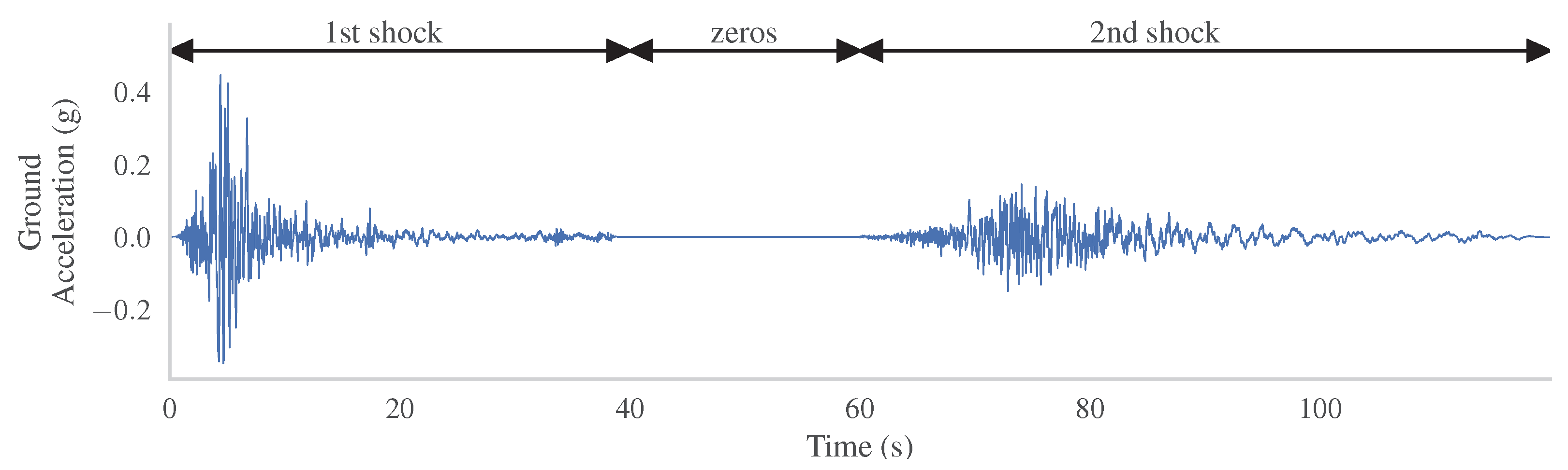
2.1. Ground Motion Records

For the purpose of this study, both artificial and natural seismic sequences are considered. By this, a sufficient set of data is ensured. Randomized seismic sequences are synthesized using a suite of 318 individual natural acceleration records to generate artificial seismic sequences accelerograms, taking into account the differences of the ground motion features [33]. The descriptive statistics of the aforementioned excitation suite are listed in

Table A1. Descriptive statistics for the IMs of the 318 individual records.

								$\mathbf{SMD}$
	$\mathbf{PGA}$	$\mathbf{PGV}$	$\mathbf{PGD}$	${\mathbf{I}}_{\mathbf{A}}$	$\mathbf{CAV}$	${\displaystyle \frac{\mathbf{PGA}}{\mathbf{PGV}}}$	${\mathbf{I}}_{\mathbf{AS}}$	$\mathbf{TB}$	$\mathbf{ROG}$	$\mathbf{Bolt}$	${\mathbf{P}}_{\mathbf{90}}$	${\mathbf{a}}_{\mathbf{rms}}$	${\mathbf{I}}_{\mathbf{c}}$	${\mathbf{I}}_{\mathbf{FVF}}$	${\mathbf{I}}_{\mathbf{RG}}$	${\mathbf{SI}}_{\mathbf{H}}$
	$\frac{\mathrm{cm}}{{\mathbf{s}}^2}$	$\frac{\mathrm{cm}}{\mathbf{s}}$	cm	$\frac{\mathrm{cm}}{\mathbf{s}}$	$\frac{\mathrm{cm}}{\mathbf{s}}$	${\mathbf{s}}^{-1}$	$\frac{\mathrm{cm}}{\mathbf{s}}$	s	s	s	$\frac{\mathrm{cm}}{{\mathbf{s}}^2}$	$\frac{\mathrm{cm}}{{\mathbf{s}}^2}$	$\frac{{\mathrm{cm}}^{1.5}}{{\mathbf{s}}^{2.5}}$	$\mathrm{cm}·{\mathbf{s}}^{-0.75}$	$\mathrm{cm}·{\mathbf{s}}^{\frac{1}{3}}$	cm
$\mu$	302.5	29.5	52.0	134.1	754.4	12.9	3.5	13.8	17.2	12.0	16.0	76.8	2301.9	53.4	143.2	91.8
$\sigma$	247.5	24.4	124.7	186.4	516.5	8.5	5.0	10.0	11.3	10.0	26.2	63.9	2455.5	42.1	398.7	72.8
min	32.7	1.2	0.1	0.7	28.0	1.7	0.0	0.6	1.9	0.0	0.1	7.4	55.3	1.4	0.1	2.1
max	1465.2	132.8	1314.2	1332.4	3119.3	75.5	41.5	49.5	56.9	58.6	150.1	306.4	13,323.4	201.8	4625.5	387.1

(Appendix A). In order to construct the artificial seismic sequences, composed of two successive seismic records, every record of the aforementioned suite is combined randomly in pairs with another six records record of the same suite. Thus, six individual seismic sequences comprised of the same main-shock are generated. As a result, 1908 pairs of first and second shock are constructed. These seismic sequences and the corresponding structural responses are used as the major part of the overall dataset for the specific ML problem. As a minor part of the overall dataset, 111 natural pairs of sequential shock records are considered. The assumed natural sequences are occurred from 1972 to 2020, while the time gap between the occurrence of the successive shocks is smaller than fifteen months. It has to be mentioned that each mainshock-aftershock record is obtained by the same station. As a result, the natural set consisted of 41 real seismic sequences recorded by 63 stations. Both sequential and individual records are selected from the ESM [34] and PEER NGA West [35] databases. The natural seismic sequences are listed in

Table A2. Seismic metadata for natural sequences.

Region	1st Shock		2nd Shock		Station Code/Name	Component	PGA${}_{1\mathbf{st}}$ (g)	PGA${}_{2\mathbf{nd}}$ (g)
	Date	M	Date	M
Ancona	14-06-1972	4.2	21-06-1972	4.0	ANP	N-S	0.220	0.410
Friuli	11-09-1976	5.8	15-09-1976	6.1	BUI	N-S	0.233	0.110
						E-W	0.108	0.093
					GMN	N-S	0.328	0.324
						E-W	0.299	0.644
Montenegro	15-04-1979	6.9	15-04-1979	5.8	PETO	E-W	0.304	0.089
			24-05-1979	6.2	BAR	N-S	0.371	0.201
						E-W	0.360	0.267
					HRZ	N-S	0.215	0.066
						E-W	0.254	0.076
					ULO	N-S	0.282	0.033
						E-W	0.236	0.030
Imperial Valley	15-10-1979	6.5	15-10-1979	5.0	Holtville Post Office	315	0.221	0.254
Mammoth Lakes	25-05-1980	6.1	25-05-1980	5.7	Convict Creek	90	0.419	0.371
Irpinia	23-11-1980	6.9	24-11-1980	5.0	BGI	N-S	0.129	0.031
						E-W	0.189	0.033
					STR	N-S	0.224	0.018
						E-W	0.320	0.032
Gulf of Corinth	24-02-1981	6.6	25-02-1981	6.3	KORA	Trans	0.296	0.121
						Logn	0.240	0.121
Coalinga	22-07-1983	5.8	25-07-1983	5.2	Elm (Old CHP)	90	0.519	0.677
						0	0.341	0.481
Kalamata	13-09-1986	5.9	15-09-1986	4.8	KAL1	Trans	0.269	0.140
						Logn	0.232	0.237
					KALA	Trans	0.296	0.152
						Logn	0.216	0.334
Spitak	07-12-1988	6.7	07-12-1988	5.9	GUK	N-S	0.181	0.144
						E-W	0.182	0.099
	08-01-1989	4.0	08-01-1989	4.1	NAB	E-W	0.206	0.217
Georgia	03-05-1991	5.6	03-05-1991	5.2	SAMB	N-S	0.354	0.208
						E-W	0.504	0.122
Erzican	13-03-1992	6.6	15-03-1992	5.9	AI 178 ERC MET	N-S	0.411	0.032
						E-W	0.487	0.039
Ilia	26-03-1993	4.7	26-03-1993	4.9	PYR1	Logn	0.109	0.100
Northridge	17-01-1994	6.7	17-01-1994	5.9	Moorpark—Fire Station	90	0.193	0.139
						180	0.291	0.184
			17-01-1994	5.2	Pacoima Kagel Canyon	360	0.432	0.053
			20-03-1994	5.3	Rinaldi Receiving Station	228	0.874	0.529
					Sepulveda Hospital	270	0.752	0.102
					Sylmar-Olive Med	90	0.605	0.181
Umbria Marche	26-09-1997	5.7	26-09-1997	6.0	CLF	N-S	0.276	0.197
						E-W	0.256	0.227
					NCR	N-S	0.395	0.502
Kalamata	13-10-1997	6.5	18-11-1997	6.4	KRN1	Trans	0.119	0.071
						Logn	0.118	0.092
Bovec	12-04-1998	5.7	31-08-1998	4.3	FAGG	N-S	0.024	0.023
						E-W	0.023	0.026
Azores Islands	09-07-1998	6.2	11-07-1998	4.7	HOR	N-S	0.405	0.082
						E-W	0.369	0.092
Izmit	17-08-1999	7.6	12-11-1999	7.3	ARC	N-S	0.210	0.007
						E-W	0.132	0.007
					ATK	N-S	0.102	0.016
						E-W	0.167	0.016
					DHM	N-S	0.090	0.017
						E-W	0.084	0.017
					FAT	N-S	0.181	0.034
						E-W	0.161	0.024
					KMP	N-S	0.102	0.014
						E-W	0.127	0.017
					ZYT	N-S	0.119	0.021
						E-W	0.109	0.029
Athens	07-09-1999	5.9	07-09-1999	4.3	SPLB	Trans	0.324	0.059
						Logn	0.341	0.071
Chi-Chi	20-09-1999	7.6	20-09-1999	6.2	TCU071	N-S	0.651	0.382
						E-W	0.528	0.193
					TCU129	N-S	0.624	0.398
						E-W	1.005	0.947
			25-09-1999	6.3	TCU078	N-S	0.307	0.387
						E-W	0.447	0.266
					TCU079	N-S	0.424	0.626
						E-W	0.592	0.776
Duzce	12-11-1999	7.3	12-11-1999	4.7	AI 010 BOL	E-W	0.820	0.060
Bingöl	01-05-2003	6.3	01-05-2003	3.5	AI 049 BNG	N-S	0.519	0.147
						E-W	0.291	0.068
L Aquila	06-04-2009	6.1	07-04-2009	5.5	AQK	N-S	0.353	0.081
						E-W	0.330	0.090
					AQV	N-S	0.545	0.146
						E-W	0.657	0.129
					AVZ	N-S	0.069	0.021
			09-04-2009	5.4	AQA	N-S	0.442	0.057
Darfield	03-09-2010	7.0	21-02-2011	6.2	Botanical Gardens	S01W	0.190	0.452
						N89W	0.155	0.552
					Cashmere High School	S80E	0.251	0.349
					Cathedral College	N26W	0.194	0.384
						N64E	0.233	0.478
					Christchurch Hospital	N01W	0.209	0.346
						S89W	0.152	0.363
Emilia	20-05-2012	6.1	29-05-2012	6.0	MRN	N-S	0.263	0.294
						E-W	0.262	0.222
	03-06-2012	5.1	12-06-2012	4.9	T0827	N-S	0.490	0.585
						E-W	0.263	0.234
Central Italy	24-08-2016	6.0	24-08-2016	5.4	AQK	E-W	0.050	0.010
			26-08-2016	4.8	AMT	N-S	0.375	0.336
						E-W	0.867	0.325
	26-10-2016	5.4	26-10-2016	5.9	CMI	N-S	0.341	0.308
						E-W	0.720	0.651
					CNE	E-W	0.556	0.537
			30-10-2016	6.5	CIT	N-S	0.052	0.213
						E-W	0.092	0.325
	26-10-2016	5.9	30-10-2016	6.5	CLO	N-S	0.193	0.582
						E-W	0.183	0.427
					CNE	N-S	0.380	0.294
					MMO	N-S	0.168	0.188
						E-W	0.170	0.189
					NOR	E-W	0.215	0.311
	30-10-2016	6.5	31-10-2016	4.2	T1213	N-S	0.867	0.185
						E-W	0.794	0.212
	18-01-2017	5.5	18-01-2017	5.4	PCB	N-S	0.586	0.561
						E-W	0.408	0.388
Dodecanese Islands	08-08-2019	4.8	30-10-2020	7.0	GMLD	N-S	0.450	0.899
						E-W	0.673	0.763

(Appendix A). Both in the case of artificial and natural seismic sequences, an intermediate zero-ceasing time gap of 20 s is added between the two successive records (Figure 1). By this, the overlap between the building oscillations is eliminated. It should be noted that nonlinear time history analyses (NLTHAs) are performed not only using the seismic sequences but also using the first shock of each sequence, as the scope of this study is to examine the seismic structural response not only under seismic sequences but also under single ground motion records.

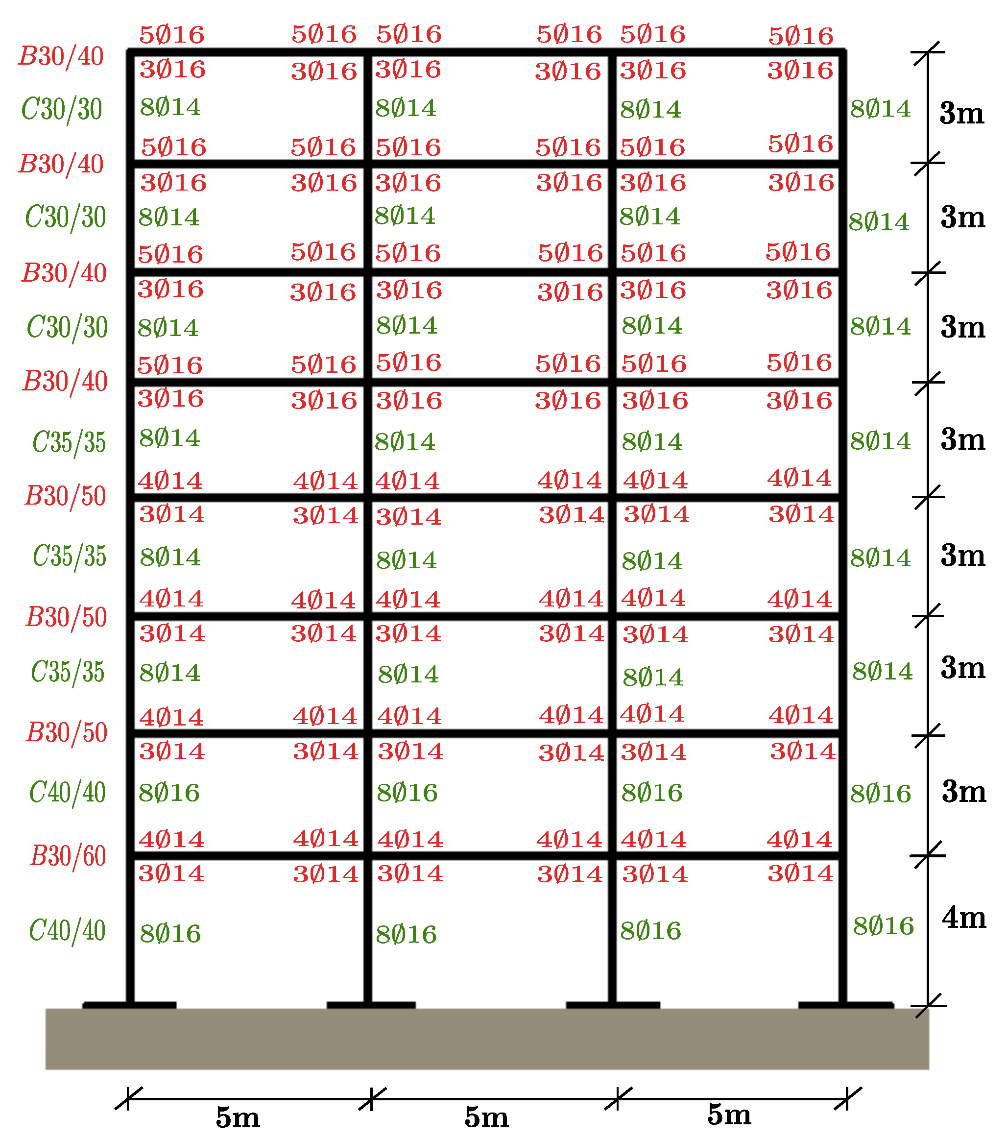
2.2. Reinforced Concrete Structure

Existing buildings designed and constructed without earthquake provisions comprise the majority of structures both in Greece and worldwide. That fact raises particular concern about their response to a potential earthquake. In this view, an 8-storey planar regular RC frame (Figure 2) designed only for gravity loads by Hatzigeorgiou and Liolios [9] is examined in the present study. The finite element simulation of the frame is conducted in IDARC 2D [36] using the spread plasticity concept and the three-parameter Park hysteretic model [37]. Every floor is considered to have only one horizontal degree of freedom to take into account the huge plane stiffness of RC slabs as a rigid diaphragm. Sparsely placed stirrups with poor anchor details are assumed in order to be in accordance with obsolete design codes. Thus, a nonlinear deformation-stress model for concrete without confinement is adopted. As a result, the concrete with a mean compressive strength equal to 28 MPa is modeled by a curve defined by the initial modulus of elasticity (${\mathrm{E}}_{\mathrm{0}}=31.42$ GPa), the strain at the maximum stress (${ϵ}_{\mathrm{c}\mathrm{0}}=2‰$), the ultimate strain in compression (${ϵ}_{\mathrm{c}\mathrm{u}}=3.5‰$), stress at tension cracking ${\sigma }_{\mathrm{t}}=0.0022$ GPa, and slope of the post-peak falling branch (${\mathrm{E}}_{\mathrm{f}\mathrm{b}}=-6.2$ GPa). Furthermore, for steel grade S500s a bilinear curve with hardening was employed. The yield and ultimate strengths were equal to 550 MPa and 660 MPa, respectively, and the corresponding strains equal to $2.75‰$ and 45‰, according to Eurocode-2 [38] provisions. The initial elastic fundamental period of the structure is equal to 1.27 s. The generation of IDARC 2D input files and the post-processing of the results are performed through GNU Octave [39,40] code.

3. Features, Targets and Dataset Generation

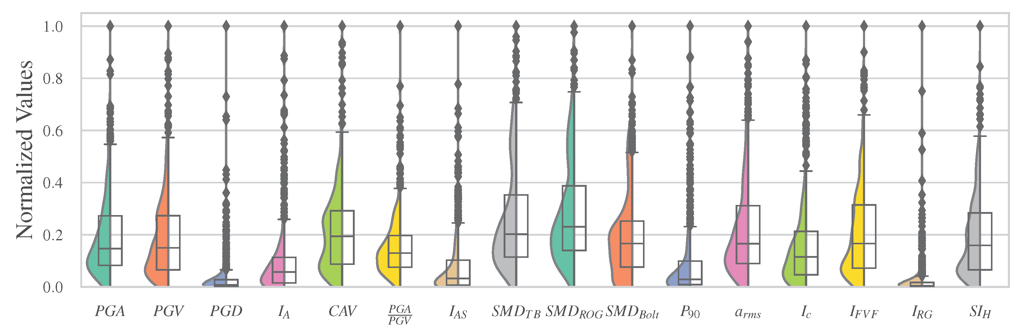
3.1. Ground Motion IMs

The basic parameters adopted in order to perform a seismic structural damage prediction analysis are the characteristics of the ground motion. By this, the identification of the seismic parameters that affect the dynamic response is of utmost importance. For this purpose, a set of 16 ground motion IMs is calculated. Amplitude parameters such as the maximum absolute values of ground accelerations (${\mathrm{a}}_{\mathrm{g}}\left(\mathrm{t}\right)$), velocities (${\mathrm{v}}_{\mathrm{g}}\left(\mathrm{t}\right)$), and displacement (${\mathrm{d}}_{\mathrm{g}}\left(\mathrm{t}\right)$) signals, which were referenced as PGA, PGV, and PGD [41], respectively, are examined. Additionally, the Arias intensity (${\mathrm{I}}_{\mathrm{A}}$) [42] and the cumulative absolute velocity (CAV) [43], which are calculated by the integral of the accelerogram time history, are considered.

An inherent feature of signals is the frequency content, which varies dynamically over time in the case of ground motion records. However, it can be quantified using the equivalent frequency $\mathrm{P}\mathrm{G}\mathrm{A}/\mathrm{P}\mathrm{G}\mathrm{V}$ [41] as if it was a sinusoid signal. Another quantity that is related to the frequency content of a ground motion is the potential destructiveness measure after Araya and Saragoni (${\mathrm{I}}_{\mathrm{A}\mathrm{S}}$) [44], determined by the zero-crossing number of the acceleration signal (${\mathrm{u}}_{\mathrm{o}}$) per unit of time.

Various definitions have been given in the past for the strong motion duration of a seismic excitation in order to identify the time interval of the signal in which the vast amount of its total intensity is released. In this work, the strong motion durations defined by Trifunac and Brady ($\mathrm{S}\mathrm{M}{\mathrm{D}}_{\mathrm{T}\mathrm{B}}$) [45] and by Reinoso, Ordaz and Guerrero ($\mathrm{S}\mathrm{M}{\mathrm{D}}_{\mathrm{R}\mathrm{O}\mathrm{G}}$) [46] are assumed. Both of these are based on the time evolution of Arias intensity according to the Husid diagram [47]. Additionally, the bracketed duration as described by Bolt ($\mathrm{S}\mathrm{M}{\mathrm{D}}_{\mathrm{B}\mathrm{o}\mathrm{l}\mathrm{t}}$) [48], which is defined by the first and last exceedance of 5 percent of g, is employed.

Combining the above parameters results in more complex measures such as power ${\mathrm{P}}_{90}$ [41], ${\mathrm{a}}_{\mathrm{r}\mathrm{m}\mathrm{s}}$ [41], characteristic intensity (${\mathrm{I}}_{\mathrm{c}}$) [41], the potential damage measure according to Fajfar, Vidic and Fischinger (${\mathrm{I}}_{\mathrm{F}\mathrm{V}\mathrm{F}}$) [49] and the IM after Riddell and Garcia (${\mathrm{I}}_{\mathrm{R}\mathrm{G}}$) [50].

It has to be mentioned that seismic parameters that depend on the fundamental structural period, such as individual spectral values, were not calculated. These parameters could not be used due to the elongation of the elastic period during the first seismic event. Instead, the Housner intensity [51] ($\mathrm{S}{\mathrm{I}}_{\mathrm{H}}$) which accumulates pseudo-spectral velocities (PSV) to a constant range of possible eigen periods and demonstrates high correlation with the structural damage [23,52,53] is employed. All of the mathematical expressions of the examined IMs are summarised in

Table 1. Mathematical expressions of IMs.

Num	Name	Expression	Ref.	Num	Name	Expression	Ref.
1	$\mathrm{P}\mathrm{G}\mathrm{A}$	$\mathrm{m}\mathrm{a}\mathrm{x}|{\mathrm{a}}_{\mathrm{g}}\left(\mathrm{t}\right)|$	[41]	9	$\mathrm{S}\mathrm{M}{\mathrm{D}}_{\mathrm{R}\mathrm{O}\mathrm{G}}$	$\mathrm{t}({\mathrm{H}}_{\mathrm{d}}=97.5\%)-\mathrm{t}({\mathrm{H}}_{\mathrm{d}}=2.5\%)$	[46]
2	$\mathrm{P}\mathrm{G}\mathrm{V}$	$\mathrm{m}\mathrm{a}\mathrm{x}|{\mathrm{v}}_{\mathrm{g}}\left(\mathrm{t}\right)|$	[41]	10	$\mathrm{S}\mathrm{M}{\mathrm{D}}_{\mathrm{B}\mathrm{o}\mathrm{l}\mathrm{t}}$	${\mathrm{t}}_{\mathrm{l}\mathrm{a}\mathrm{s}\mathrm{t}}^{{\mathrm{a}}_{\mathrm{g}}>0.05\mathrm{g}}-{\mathrm{t}}_{1\mathrm{s}\mathrm{t}}^{{\mathrm{a}}_{\mathrm{g}}>0.05\mathrm{g}}$	[48]
3	$\mathrm{P}\mathrm{G}\mathrm{D}$	$\mathrm{m}\mathrm{a}\mathrm{x}|{\mathrm{d}}_{\mathrm{g}}\left(\mathrm{t}\right)|$	[41]	11	${\mathrm{P}}_{90}$	$\frac{{\mathrm{I}}_{\mathrm{A}}({\mathrm{H}}_{\mathrm{d}}=95\%)-{\mathrm{I}}_{\mathrm{A}}({\mathrm{H}}_{\mathrm{d}}=5\%)}{\mathrm{S}\mathrm{M}{\mathrm{D}}_{\mathrm{T}\mathrm{B}}}$	[41]
4	${\mathrm{I}}_{\mathrm{A}}$	$\frac{\pi }{2\mathrm{g}}{\int }_{\mathrm{0}}^{{\mathrm{t}}_{\mathrm{e}\mathrm{n}\mathrm{d}}}{\mathrm{a}}_{\mathrm{g}}^2\left(\mathrm{t}\right)\mathrm{d}\mathrm{t}$	[42]	12	${\mathrm{a}}_{\mathrm{r}\mathrm{m}\mathrm{s}}$	$\sqrt{\frac{1}{\mathrm{S}\mathrm{M}{\mathrm{D}}_{\mathrm{T}\mathrm{B}}}{\int }_{{\mathrm{t}}_{5\%}}^{{\mathrm{t}}_{95\%}}{\mathrm{a}}_{\mathrm{g}}{\left(\mathrm{t}\right)}^2\mathrm{d}\mathrm{t}}$	[41]
5	$\mathrm{C}\mathrm{A}\mathrm{V}$	${\int }_{\mathrm{o}}^{{\mathrm{t}}_{\mathrm{e}\mathrm{n}\mathrm{d}}}\left|{\mathrm{a}}_{\mathrm{g}}\left(\mathrm{t}\right)\right|\mathrm{d}\mathrm{t}$	[41]	13	${\mathrm{I}}_{\mathrm{c}}$	${\mathrm{a}}_{\mathrm{r}\mathrm{m}\mathrm{s}}^{1.5}·\mathrm{S}\mathrm{M}{\mathrm{D}}_{\mathrm{T}\mathrm{B}}^{0.5}$	[41]
6	$\mathrm{P}\mathrm{G}\mathrm{A}/\mathrm{P}\mathrm{G}\mathrm{V}$	$\frac{\mathrm{P}\mathrm{G}\mathrm{A}}{\mathrm{P}\mathrm{G}\mathrm{V}}$	[41]	14	${\mathrm{I}}_{\mathrm{F}\mathrm{V}\mathrm{F}}$	$\mathrm{P}\mathrm{G}\mathrm{V}·\mathrm{S}\mathrm{M}{\mathrm{D}}_{\mathrm{T}\mathrm{B}}^{0.25}$	[49]
7	${\mathrm{I}}_{\mathrm{A}\mathrm{S}}$	$\frac{{\mathrm{I}}_{\mathrm{A}}}{{\mathrm{u}}_{\mathrm{o}}^2}$	[44]	15	${\mathrm{I}}_{\mathrm{R}\mathrm{G}}$	$\mathrm{P}\mathrm{G}\mathrm{D}·\mathrm{S}\mathrm{M}{\mathrm{D}}_{\mathrm{T}\mathrm{B}}^{\frac{1}{3}}$	[50]
8	$\mathrm{S}\mathrm{M}{\mathrm{D}}_{\mathrm{T}\mathrm{B}}$	$\mathrm{t}({\mathrm{H}}_{\mathrm{d}}=95\%)-\mathrm{t}({\mathrm{H}}_{\mathrm{d}}=5\%)$	[45]	16	$\mathrm{S}{\mathrm{I}}_{\mathrm{H}}$	${\int }_{0.1}^{2.5}\mathrm{P}\mathrm{S}\mathrm{V}(\mathrm{T},\xi =0.05)\mathrm{d}\mathrm{T}$	[51]

. The elastic spectra are defined using OpenSeismoMatlab [54], while values of the IMs are computed through Python [55] code.

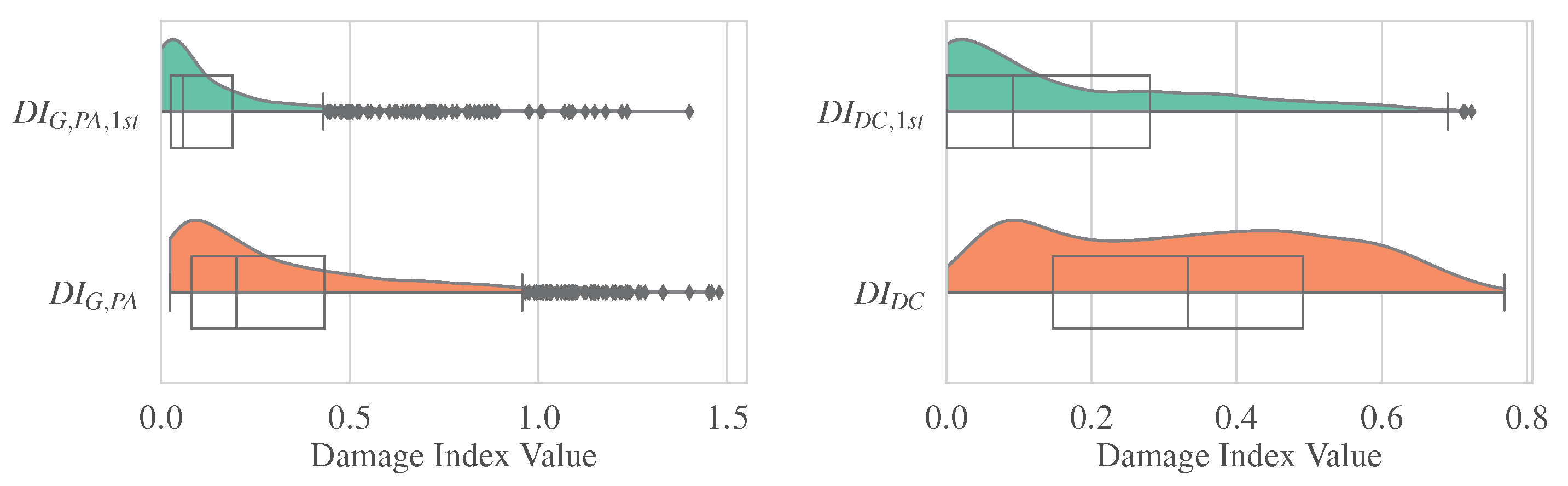
3.2. Damage Indicators

For the ML modeling of the present study, the structural damage is assumed both as an input feature to take into account the initial damage due to the former seismic shock, as well as a target feature in order to describe the damage accumulation after the examined ground motion. The structural response is assessed in terms of two overall seismic damage indices, namely, the overall damage index after Park and Ang ($\mathrm{D}{\mathrm{I}}_{\mathrm{G},\mathrm{P}\mathrm{A}}$) [36] and the damage index after DiPasquale and Çakmak ($\mathrm{D}{\mathrm{I}}_{\mathrm{D}\mathrm{C}}$) [56].

The originally introduced damage index after Park and Ang ($\mathrm{D}{\mathrm{I}}_{\mathrm{P}\mathrm{A}}$) [57] results from summation of the maximum flexural responses and the hysteretic energy consumption of the plastic hinges and is calculated by Equation (1) modified by Kunnath et al. [58] (Equation (2)). The overall damage index ($\mathrm{D}{\mathrm{I}}_{\mathrm{G},\mathrm{P}\mathrm{A}}$) [36] is calculated as a weighted average of the sub-factors, weighted by the percentages of the total energy consumed by each member of the construction, according to Equation (3). The value of $\mathrm{D}{\mathrm{I}}_{\mathrm{G},\mathrm{P}\mathrm{A}}$ as close to zero as possible implies a complete damage-free structural system with an elastic response. However, a structure is characterized as near to collapse when $\mathrm{D}{\mathrm{I}}_{\mathrm{G},\mathrm{P}\mathrm{A}}$ takes values over the unit.

$$\mathrm{D}{\mathrm{I}}_{\mathrm{P}\mathrm{A}}=\frac{{\delta }_{\mathrm{m}}}{{\delta }_{\mathrm{u}}}+\frac{\beta }{{\mathrm{Q}}_{\mathrm{y}}{\delta }_{\mathrm{u}}}\int \mathrm{d}\mathrm{E}$$

(1)

$$\mathrm{D}{\mathrm{I}}_{\mathrm{P}\mathrm{A},\mathrm{c}\mathrm{o}\mathrm{m}\mathrm{p}\mathrm{o}\mathrm{n}\mathrm{e}\mathrm{n}\mathrm{t}}=\frac{{\theta }_{\mathrm{m}}-{\theta }_{\mathrm{r}}}{{\theta }_{\mathrm{u}}-{\theta }_{\mathrm{r}}}+\frac{\beta }{{\theta }_{\mathrm{u}}{\mathrm{M}}_{\mathrm{y}}}{\mathrm{E}}_{\mathrm{h}}$$

(2)

$$\mathrm{D}{\mathrm{I}}_{\mathrm{G},\mathrm{P}\mathrm{A}}=\frac{\sum {\mathrm{E}}_{\mathrm{i}}\mathrm{D}{\mathrm{I}}_{\mathrm{P}\mathrm{A},\mathrm{c}\mathrm{o}\mathrm{m}\mathrm{p}\mathrm{o}\mathrm{n}\mathrm{e}\mathrm{n}\mathrm{t}}}{\sum {\mathrm{E}}_{\mathrm{i}}}$$

(3)

where ${\delta }_{\mathrm{m}}$ is the maximum element displacement response, ${\delta }_{\mathrm{u}}$ is the ultimate element displacement, $\beta$ is the model constant parameter for strength deterioration proposed by Park et al. [59], $\int \mathrm{d}\mathrm{E}$ is the cumulative hysteretic energy consumed by the element during its response, ${\mathrm{Q}}_{\mathrm{y}}$ is the yield strength of the element, ${\theta }_{\mathrm{m}}$ is the maximum element rotation during the time history response, ${\theta }_{\mathrm{u}}$ is the ultimate capacity of the element and ${\theta }_{\mathrm{r}}$ is the recoverable element rotation during unloading.

During high-intensity seismic events, it is known that the cross-sections in plastic hinge areas of a building can be severely cracked or even present steel yielding, resulting in structural stiffness degradation. Therefore, an increase in the building’s flexibility, and as such its fundamental period, is expected [60]. The $\mathrm{D}{\mathrm{I}}_{\mathrm{D}\mathrm{C}}$ is based on the above-mentioned increase in the fundamental period and is calculated according to Equation (4).

$$\mathrm{D}{\mathrm{I}}_{\mathrm{D}\mathrm{C}}=1-\frac{{\mathrm{T}}_{{\mathrm{0}}_{\mathrm{i}\mathrm{n}\mathrm{i}\mathrm{t}\mathrm{i}\mathrm{a}\mathrm{l}}}}{{\mathrm{T}}_{{\mathrm{0}}_{\mathrm{e}\mathrm{q}\mathrm{u}\mathrm{i}\mathrm{v}\mathrm{a}\mathrm{l}\mathrm{e}\mathrm{n}\mathrm{t}}}}$$

(4)

where ${\mathrm{T}}_{{\mathrm{0}}_{\mathrm{i}\mathrm{n}\mathrm{i}\mathrm{t}\mathrm{i}\mathrm{a}\mathrm{l}}}$ is the fundamental period before the start of the analysis, and ${\mathrm{T}}_{{\mathrm{0}}_{\mathrm{e}\mathrm{q}\mathrm{u}\mathrm{i}\mathrm{v}\mathrm{a}\mathrm{l}\mathrm{e}\mathrm{n}\mathrm{t}}}$ is the fundamental period at the end of the analysis.

3.3. Dataset Configuration

The scope of this study is to examine the capability of MLAs in predicting the structural damage of a certain RC frame under single or multiple ground motion records. To achieve this, the intensity of each seismic event and the corresponding response is treated individually, taking into account the initial structural damage just before the certain oscillation. In case of sequential seismic events, the damage incurred by the fist shock is considered to be the initial damage of the structure subjected to the aftershock. In order to provide a universal model that can predict the structural damage, regardless of the pre-earthquake state of the building, the initial damage is taken into account even if the structure is intact, i.e., in case of single seismic events. In such a case, the value of the damage indices is set as zero. It has to be mentioned that from the initial 1908 artificially generated sequences, ultimately, 1528 of them are considered. The rest of the sequences are omitted either due to convergence problems of the NLTHAs or due to the absence of structural damage under the first shock. Thus, the dataset in total comprises 1528 artificial and 111 natural seismic sequences. Additionally, 429 single seismic events are considered. As such, 2068 data instances are assumed.

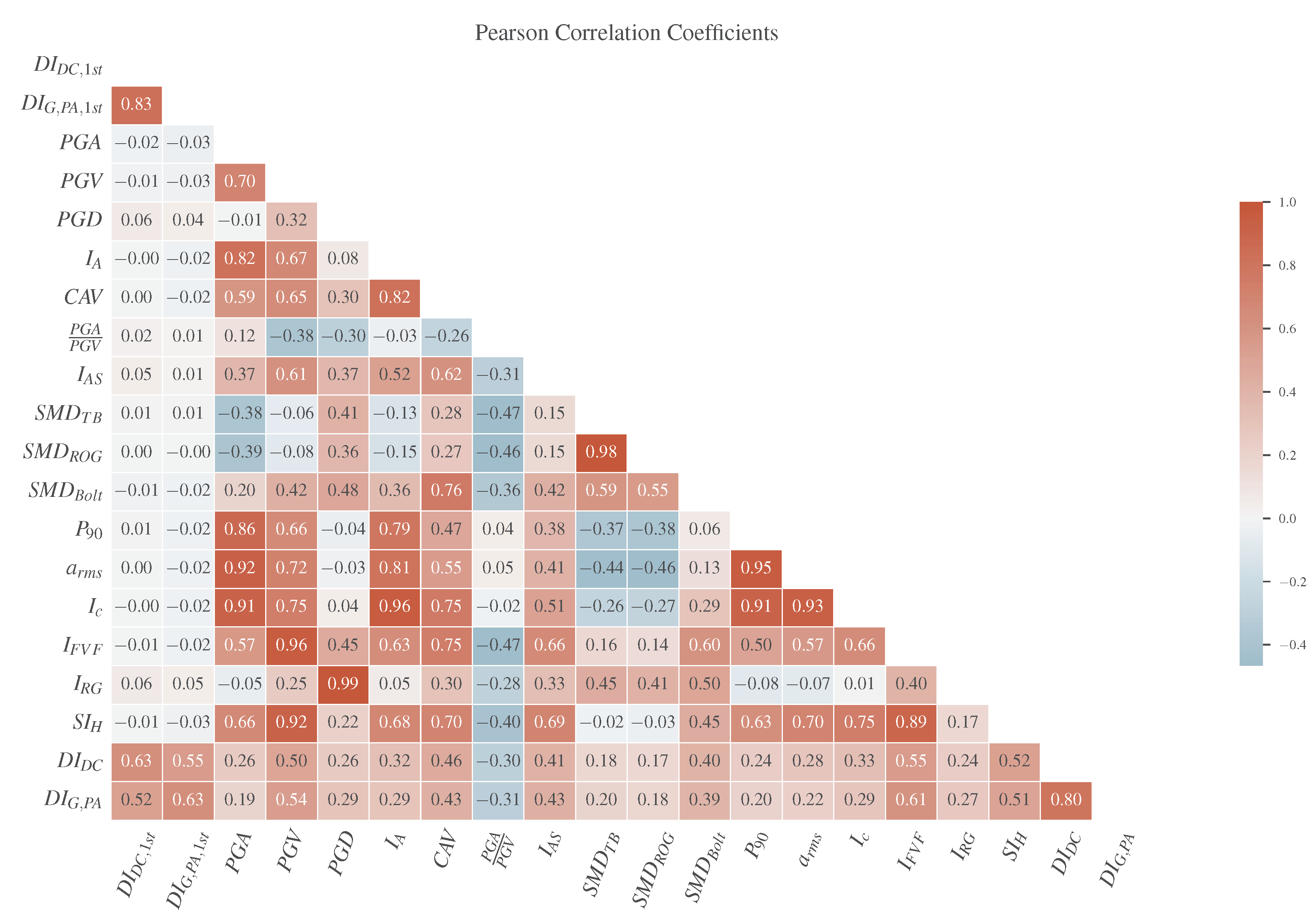
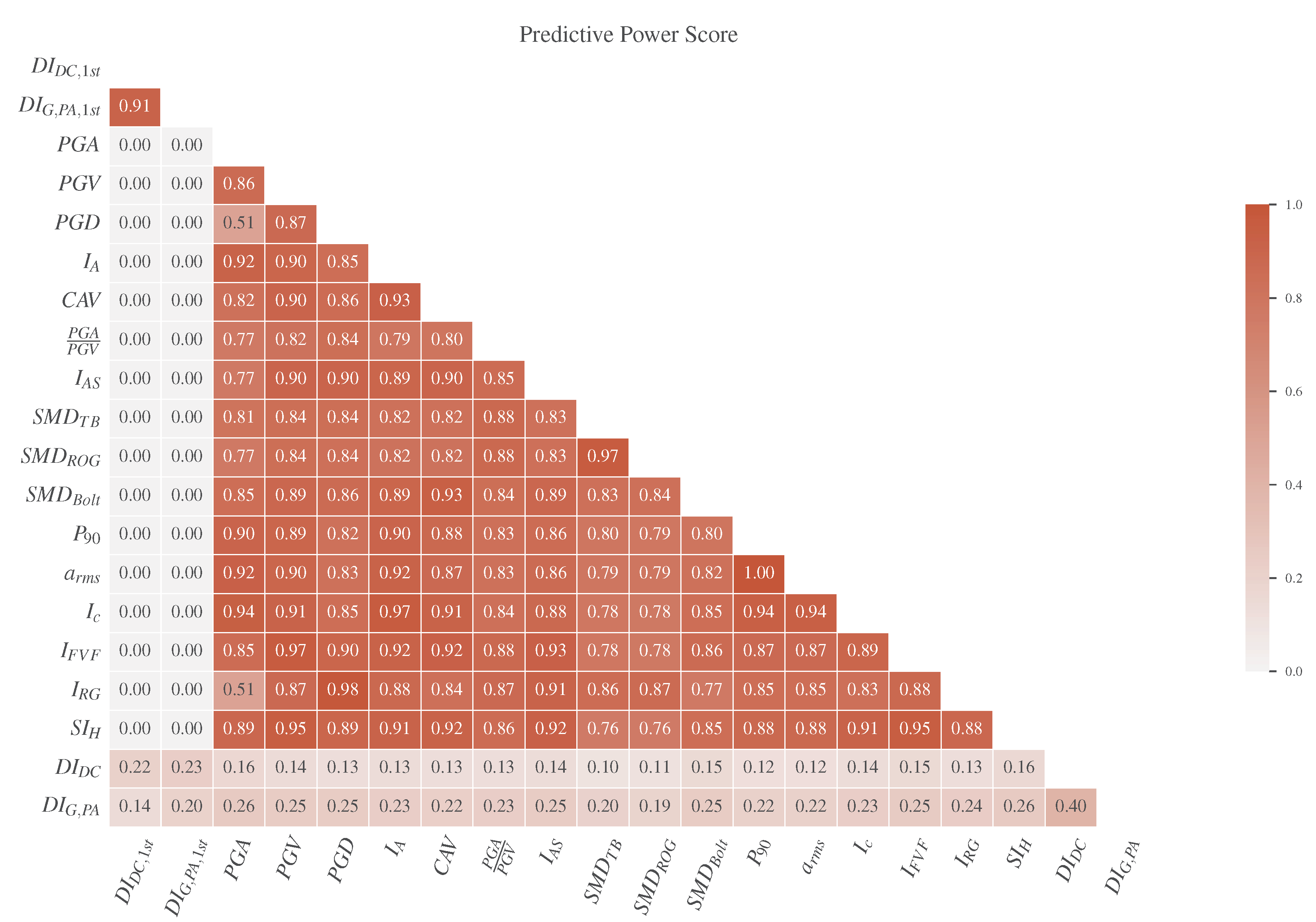
4. Exploratory Data Analysis (EDA)

For the most complete and effective decision-making, statistical analysis of the examined data is required in order to capture the technical characteristics of the problem. This exploratory analysis includes a set of numerical and graphical methods, which allow us to obtain an initial consideration about the features of the data that will be used in the ML models. The purpose of the aforementioned analysis is the practical (non-scientific) interpretation of the data by unveiling the main characteristics of the data format, as well as their origin. This technique is a necessary step before the application of statistical inference methods, in order to thoroughly check the suitability of the data, the formulation of the adopted hypotheses and the selection of the appropriate method.

In particular, based on the problem analyzed in this paper, problematic values can be identified, i.e., values that are cut off from the main corpus and can be characterized as outliers or even incorrect, and appropriately treated. Moreover, the normality of the data population can be checked. This is particularly important as many of the implemented methods require normality of the data.

Table 2. Descriptive statistics for the IMs of the overall dataset.

								$\mathbf{SMD}$
	$\mathbf{PGA}$	$\mathbf{PGV}$	$\mathbf{PGD}$	${\mathbf{I}}_{\mathbf{A}}$	$\mathbf{CAV}$	${\displaystyle \frac{\mathbf{PGA}}{\mathbf{PGV}}}$	${\mathbf{I}}_{\mathbf{AS}}$	$\mathbf{TB}$	$\mathbf{ROG}$	$\mathbf{Bolt}$	${\mathbf{P}}_{\mathbf{90}}$	${\mathbf{a}}_{\mathbf{rms}}$	${\mathbf{I}}_{\mathbf{c}}$	${\mathbf{I}}_{\mathbf{FVF}}$	${\mathbf{I}}_{\mathbf{RG}}$	${\mathbf{SI}}_{\mathbf{H}}$
	$\frac{\mathrm{cm}}{{\mathbf{s}}^2}$	$\frac{\mathrm{cm}}{\mathbf{s}}$	cm	$\frac{\mathrm{cm}}{\mathbf{s}}$	$\frac{\mathrm{cm}}{\mathbf{s}}$	${\mathbf{s}}^{-1}$	$\frac{\mathrm{cm}}{\mathbf{s}}$	s	s	s	$\frac{\mathrm{cm}}{{\mathbf{s}}^2}$	$\frac{\mathrm{cm}}{{\mathbf{s}}^2}$	$\frac{{\mathrm{cm}}^{1.5}}{{\mathbf{s}}^{2.5}}$	$\mathrm{cm}·{\mathbf{s}}^{-0.75}$	$\mathrm{cm}·{\mathbf{s}}^{\frac{1}{3}}$	cm
$\mu$	299.6	29.1	49.4	131.7	738.7	13.0	3.4	13.5	16.9	11.6	15.8	76.4	2267.1	52.4	135.1	90.4
$\sigma$	244.1	24.2	120.6	186.2	527.0	8.6	5.0	10.0	11.3	10.0	25.9	63.5	2430.7	42.3	383.3	73.3
min	7.4	0.8	0.0	0.2	28.0	1.7	0.0	0.5	0.7	0.0	0.0	1.8	12.5	1.4	0.1	1.5
max	1465.2	148.2	1314.2	1332.4	3354.8	75.5	41.5	49.5	56.9	58.6	170.7	326.2	13,323.4	243.0	4625.5	457.7

lists the most important statistics of the ground motions’ IMs. The mean ($\mu$) of a population estimates the median value for symmetric or nearly symmetric distributions. Additionally, $\sigma$ estimates the standard deviation in the population. When the standard deviation is elevated, we know that there are values of the variable sufficiently far from the mean. In a normal distribution, 95% of the values of the variable are within the limits $\mu \pm 2\sigma$. Moreover, the minimum (min) and the maximum (max) values of each variable indicate the wide range of the seismic parameters.

The statistical representation of the data is shown in Figure 3 and Figure 4, where clear information is provided about the centre of the data, the symmetry, the skewness, the type of any asymmetry and the outliers. Information on the distortion and curvature of the distribution is also sought. Distortion refers to any deviation over the normal distribution. If the curve shifts to the left or right, it is said to be skewed. Skewness can be quantified as a representation of the degree to which a given distribution differs from a normal distribution. A normal distribution is non-skewed, while, for example, a lognormal distribution exhibits right skewness. Distributions can exhibit right (positive) skewness or left (negative) skewness in varying degrees. The skewness is the degree of asymmetry that is observed in a probability distribution. A distribution with positive asymmetry possesses a shift to a median with lower values. Obviously, the opposite is true in the case of negative asymmetry.

In Figure 3, the distributions of all the examined IMs with their values normalized in (0, 1) are presented. Moreover, in Figure 4, the distribution of the structural damage after the single ($\mathrm{D}{\mathrm{I}}_{\mathrm{G},\mathrm{P}\mathrm{A},1\mathrm{s}\mathrm{t}}$, $\mathrm{D}{\mathrm{I}}_{\mathrm{D}\mathrm{C},1\mathrm{s}\mathrm{t}}$) and the successive ($\mathrm{D}{\mathrm{I}}_{\mathrm{G},\mathrm{P}\mathrm{A}}$, $\mathrm{D}{\mathrm{I}}_{\mathrm{D}\mathrm{C}}$) seismic events are depicted comparatively. Under seismic sequences, damage accumulation can be observed, as the distributions of both damage indices are shifted to higher values compared to those that correspond to the damage after the first shocks. It has been mentioned that Figure 3 and Figure 4, despite offering meaningful information, constitute a tool of data exploratory analysis without leading to definitive conclusions.

Values that are characterised as extremes or outliers are merely “suspect” values, i.e., values which may be incorrect or unusual. The number of points clarified as outliers depends on the sample size and the shape of the distribution. To identify the outliers, Cook’s distance [61,62] values were calculated according to Equation (5) and illustrated in Figure 5a,b for the $\mathrm{D}{\mathrm{I}}_{\mathrm{G},\mathrm{P}\mathrm{A}}$ and $\mathrm{D}{\mathrm{I}}_{\mathrm{D}\mathrm{C}}$ datasets, respectively. In the same figure, the threshold which is equal to ${\mathrm{I}}_{\mathrm{t}}=\frac{4}{\mathrm{n}}$ (n: number of observations) is depicted. The percentage of the potential outliers with influence that exceeds the above threshold is equal to 8.99% and 7.21% for the $\mathrm{D}{\mathrm{I}}_{\mathrm{G},\mathrm{P}\mathrm{A}}$ and $\mathrm{D}{\mathrm{I}}_{\mathrm{D}\mathrm{C}}$ datasets, respectively.

$${\mathrm{D}}_{\mathrm{i}}=\sum _{\mathrm{i}=1}^{\mathrm{n}}\frac{{({\widehat{\mathrm{y}}}_{\mathrm{j}}-{\widehat{\mathrm{y}}}_{\mathrm{j}\left(\mathrm{i}\right)})}^2}{\mathrm{p}\mathrm{M}\mathrm{S}\mathrm{E}}$$

(5)

where ${\widehat{\mathrm{y}}}_{\mathrm{j}}$ is the jth predicted value, ${\widehat{\mathrm{y}}}_{\mathrm{j}\left(\mathrm{i}\right)}$ is the jth predicted value, where the fit does not include observation i, MSE is the mean squared error, and p is the number of coefficients in the regression model.

Subsequently, a correlation analysis was carried out in order to determine the degree of linear correlation between each pair of involved variables X and Y with variances ${\sigma }_{\mathrm{X}}$ and ${\sigma }_{\mathrm{Y}}$, respectively, and covariance ${\sigma }_{\mathrm{X}\mathrm{Y}}=\mathrm{C}\mathrm{O}\mathrm{V}(\mathrm{X},\mathrm{Y})=\mathrm{E}(\mathrm{X},\mathrm{Y})-\mathrm{E}\left(\mathrm{X}\right)\mathrm{E}\left(\mathrm{Y}\right)$. The results of the calculation of the Pearson coefficient [63] according to Equation (6) are shown in Figure 6.

$${\rho }_{\mathrm{X},\mathrm{Y}}=\frac{\mathrm{C}\mathrm{O}\mathrm{V}(\mathrm{X},\mathrm{Y})}{{\sigma }_{\mathrm{X}}{\sigma }_{\mathrm{Y}}}$$

(6)

Because there is a proven inability of the Pearson method to detect nonlinear correlations such as sinusoidal waves, quadratic curves, etc., the Predictive Power Score (PPS) [64] technique was also used to summarize the predictive relationships between the available data, explaining how variable A informs variable B more than variable B informs variable A. Technically, the score is a measurement in the interval (0, 1) of the success of a model in predicting a target variable with the help of an out-of-sample predictor variable. From this method, hidden patterns of the data can be identified and as such faciliate the selection of appropriate prediction variables. The results of the PPS calculation are shown in the Figure 7.

After this analytical investigation of the data of the considered research, the analytical statistical hypothesis testing for testing hypotheses related to the distribution of X (with its unknown parameters and its shape), and hypothesis and independence testing related to the comparison of the unknown parameters of the problem variables, it was shown that this dataset is suitable for the correct application of ML methods. It is particularly important to understand the logic, meaning and limits of application of the data in question, so that this knowledge will allow us to correctly interpret the results and make correct conclusions with an awareness of the magnitude of the uncertainty in them. The logic question is directly related to the ongoing research question of whether the data used in the application being developed are appropriate and actually model the problem.

In conclusion, the above investigation allows us to interpret whether a MLA can extract a confident value associated with the option available to it. Similarly, it allows us to interpret whether it can abstain from trusting the choice when a particular output is too low. Finally, it is possible to explore algorithms that can be more effectively integrated into larger tasks in a way that partially or completely avoids the problem of error propagation.

5. Results

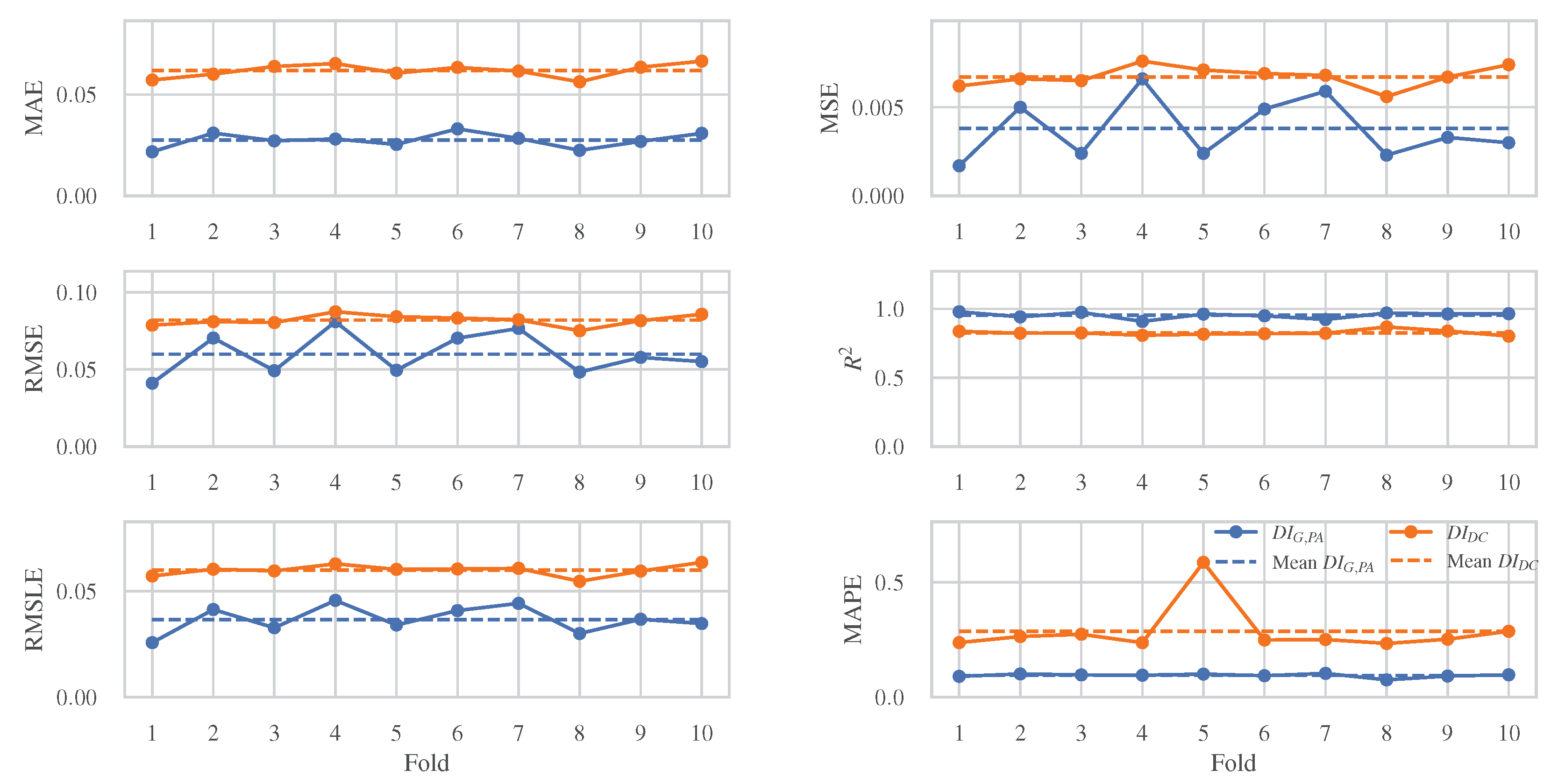
5.1. Comparative Performance Analysis of the Examined MLAs

The selection of the proper MLA in modelling the seismic demand prediction of the examined RC frame under single and multiple ground motion records is of outmost importance. This selection has to be made by taking into account the particularities of the current data, the EDA and restrictions of the examined algorithms. In order to obtain the most efficient algorithm, a thorough comparatively investigation among 10 different MLAs was performed. Their performance was assessed by conducting sensitivity and accuracy analysis regarding the estimated errors obtained by the provided data.

The ten examined MLAs are: the Adaboost regressor (ABR) [65], the Bayesian ridge (BR) [66], the decision tree regressor (DTR) [67], the extra trees regressor (ETR) [68], the gradient boosting regressor (GBR) [69], the K-nearest neighbors (KNN) [70,71], the light gradient boosting machine (LGBM) [72], the linear regressor (LR) [73], the multi-layer feed-forward neural network (MLNN) [74], and the random forest regressor (RFR) [75]. In this sense, an extensive and detailed comparison of 10 different MLAs on the two provided datasets was carried out. The MLAs are implemented using the Scikit-learn [76] and LightGBM [72] Python packages, while they are evaluated with Yellowbrick library [77,78]. It should be said that the following metrics [73] for the comparison and cost analysis of the correct regression errors were taken into account and are listed below:

• Mean absolute error (MAE) is a measure of errors between the estimated and the observed values, and it is given by the following expression:

  $$\mathrm{M}\mathrm{A}\mathrm{E}=\frac{1}{\mathrm{n}}\sum _{\mathrm{i}=1}^{\mathrm{n}}\mid {\widehat{\mathrm{y}}}_{\mathrm{i}}-{\mathrm{y}}_{\mathrm{i}}\mid$$

  (7)

  where ${\widehat{\mathrm{y}}}_{\mathrm{i}}$ is the predicted value, ${\mathrm{y}}_{\mathrm{i}}$ the real value of the ith observation and n is the total number of observations;
• Mean square error (MSE):

  $$\mathrm{M}\mathrm{S}\mathrm{E}=\frac{1}{\mathrm{n}}\sum _{\mathrm{i}=1}^{\mathrm{n}}{({\widehat{\mathrm{y}}}_{\mathrm{i}}-{\mathrm{y}}_{\mathrm{i}})}^2$$

  (8)
• Root-mean-squared error (RMSE) calculates the average error between the estimated values and the observed values:

  $$\mathrm{R}\mathrm{M}\mathrm{S}\mathrm{E}=\sqrt{\frac{1}{\mathrm{n}}\sum _{\mathrm{i}=1}^{\mathrm{n}}{({\widehat{\mathrm{y}}}_{\mathrm{i}}-{\mathrm{y}}_{\mathrm{i}})}^2}$$

  (9)
• The coefficient of determination, ${\mathrm{R}}^2$, expresses the variation in the dependent variable that is predictable from the independent variables:

  $${\mathrm{R}}^2=1-\frac{{\sum }_{\mathrm{i}=1}^{\mathrm{n}}{({\mathrm{y}}_{\mathrm{i}}-{\widehat{\mathrm{y}}}_{\mathrm{i}})}^2}{{\sum }_{\mathrm{i}=1}^{\mathrm{n}}{({\mathrm{y}}_{\mathrm{i}}-{\overline{\mathrm{y}}}_{\mathrm{i}})}^2}$$

  (10)

  where $\overline{\mathrm{y}}$ is the average of the observed values;
• Root-mean-squared-log-error (RMSLE) is an extension of MSE that is used mainly when the predicted values display high deviation:

  $$\mathrm{R}\mathrm{M}\mathrm{S}\mathrm{L}\mathrm{E}=\sqrt{\frac{1}{\mathrm{n}}\sum _{\mathrm{i}=1}^{\mathrm{n}}{(log({\widehat{\mathrm{y}}}_{\mathrm{i}}+1)-log({\mathrm{y}}_{\mathrm{i}}+1))}^2}$$

  (11)
• Mean absolute percentage error (MAPE) calculates the accuracy, as a ratio, and is defined by the following formulation:

  $$\mathrm{M}\mathrm{A}\mathrm{P}\mathrm{E}=\frac{1}{\mathrm{n}}\sum _{\mathrm{i}=1}^{\mathrm{n}}\left|\frac{{\mathrm{y}}_{\mathrm{i}}-{\widehat{\mathrm{y}}}_{\mathrm{i}}}{{\mathrm{y}}_{\mathrm{i}}}\right|$$

  (12)

In order to thoroughly assess the ML methods, 30 percent of the total dataset was withheld and was employed as a test set for the final assessment. In the remaining part, we trained and evaluated all of the examined algorithms using the K-fold cross-validation strategy [76]. During this method, the above part is divided in K subsets. Each randomly defined subset consists of different observations. One subset is used as the cross-validation subset, while the K-1 others are merged and used as the training set. This process is performed K times using different sets as the validation set and the K-1 rest of them as the training set. The performance of the MLA is evaluated for each case and on average. By this, the performance of the method in relation to the prediction error is determined. Specifically, the statistical properties, the bias and the variance of the regression prediction error are recorded and analyzed using a 10-fold cross-validation procedure. A decomposition of the variability of the 10-fold cross-validation sample is performed, taking into account its variability sources.

In Figure 8, the metrics of each MLA for both damage indices are presented. It can be seen that considering $\mathrm{D}{\mathrm{I}}_{\mathrm{G},\mathrm{P}\mathrm{A}}$, higher performance of the ML modelling is obtained. Specifically, the algorithm with the best prediction capability is the extra trees regressor. This method is based on decision trees and randomizes decision trees for random sub-samples in order to minimize over-fitting. In particular, given a data sample $\mathbf{X}={\mathbf{x}}_1,\cdots ,{\mathbf{x}}_{\mathrm{n}}$ and the respected values $\mathbf{y}={\mathrm{y}}_1,\cdots ,{\mathrm{y}}_{\mathrm{n}}$, a random sample is chosen repeatedly without substitution from the learning ensemble in order to estimate the target values using decision trees. The extra trees algorithm performs like random forest, as multiple trees are generated and the nodes are separated using randomly chosen subsets of features. However, there are two main differences: the sampling is carried out without replacement, which means that there is no bootstrap, and the nodes are separated randomly among a random subset of features that are chosen for every node. The aforementioned randomness is based on the random separations of the total sample. Thus, low variance is achieved. Another important feature is that the predictions are calculated by multiple decision trees, and as such, there is high prediction accuracy for new data. Moreover, the algorithm reduces the risk of over-fitting due to the randomness that is introduced in the model.

Considering the $\mathrm{D}{\mathrm{I}}_{\mathrm{D}\mathrm{C}}$, the algorithm with the higher prediction capacity is the gradient boosting regressor. The boosted trees algorithms are a combination of boosting and decision trees. Boosting is a meta-algorithm for reducing bias in supervised learning. In the case of boosting [79], predictive regressors are used in order to develop weighted trees. The features of the regression trees and the boosting algorithms are combined to produce boosting trees. The gradient boosting method produces a prediction model comprised of a set of weak prediction, usually decision tree, models. It builds the model gradually and generalizes it by optimizing a loss function. In other words, at each iteration, a new weak regressor is trained and the previous ones are extended in order to increase the accuracy of the model.

Based on the above observation, these algorithms could provide a generalized model that could be capable of reliably predicting the final damage of the examined RC frame for given new values, different from training ones, of the established damage and seismic shock IMs.

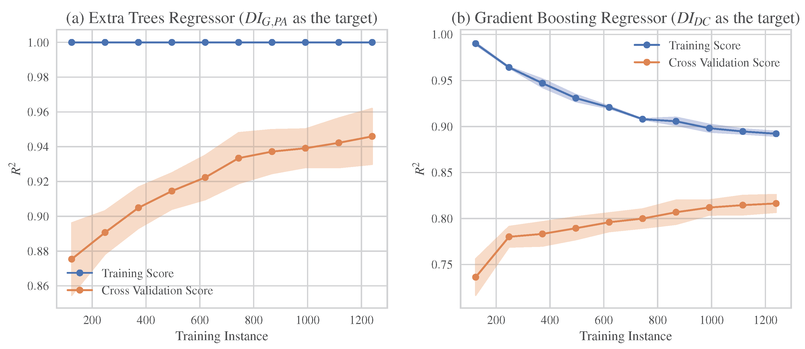
5.2. Evaluation of the MLAs with the Higher Prediction Ability

In this section, we provide a more detailed description about the performance of the MLAs with the higher prediction ability during the 10-fold procedure. In Figure 9, the error metrics are depicted comparatively for the qualified MLA of each damage index. In general, the extra trees regressor algorithm exhibits higher performance than the gradient boosting regressor algorithm considering the $\mathrm{D}{\mathrm{I}}_{\mathrm{G},\mathrm{P}\mathrm{A}}$ and $\mathrm{D}{\mathrm{I}}_{\mathrm{D}\mathrm{C}}$ structural damage indexes, respectively. Considering $\mathrm{D}{\mathrm{I}}_{\mathrm{G},\mathrm{P}\mathrm{A}}$, a generally smooth shift of the error is observed that expresses the probability of a given number of events occurring over a fixed period of time, taking into account the observations that occur at a known average constant rate and are independent of their appearance. There is only one case of significant error fluctuation which describes repetitive non-periodic alterations that could not be predicted by this algorithm. Regarding the $\mathrm{D}{\mathrm{I}}_{\mathrm{D}\mathrm{C}}$, it is observed that there is higher dispersion of the error, which normalizes in the later folds. This fact translates the randomness of the samples into some folds, which are independent of the time period of their occurrence. The normalization and stabilization of the error after the initial fluctuations describes some possible repetitive non-periodic changes which are satisfactorily predicted by the specific algorithm. By this fact, the model can calculate reliable output values for inputs that are new and different from those with which it is trained.

The 10-fold procedure is implemented iteratively in a progressively increasing subset in order to produce the learning curves. In both cross-validation and training sets, the average and the range of ${\mathrm{R}}^2$ are calculated for each iteration. A major control procedure of the adjustment and the response of the algorithms is based on the learning curve, which depicts the learning performance as a function of the gained experience. It is a widely used tool that assesses the training and the validation data after each update of the measured error performance. Via this method, problems such as under- or over-fitting of the model, and the adequacy of the training or the validation data, could emerge. In Figure 10, the learning curves of the distinctive MLA for each dataset are depicted. Specifically, Figure 10a illustrates the learning curves of the extra trees regressor algorithm when the structural damage is assessed in terms of $\mathrm{D}{\mathrm{I}}_{\mathrm{G},\mathrm{P}\mathrm{A}}$, while Figure 10b presents the learning curves of the gradient boosting regressor considering structural damage in terms of $\mathrm{D}{\mathrm{I}}_{\mathrm{D}\mathrm{C}}$.

It is obvious that the training curve of Figure 10a improves as the experience of the model increases without any trends of over-fitting. That fact could be identified by small alterations similarly presented in both training and cross-validation curves. The prediction ability of the model is highlighted due to the high performance beginning at the starting point of the procedure with a score over 0.87. An increasing trend is depicted with a rather narrow confidence interval, a fact that reflects the quality of the model. Moreover, there is no loss of the training, and as such, the distance between training and the validation curve reduces in relation to the experience. This distance is referred to as the “generalization gap” and defines the quality of the model. It is obvious that smaller gaps between the two curves implies higher accuracy of the model.

From the training and the validation curves of Figure 10b, it could be easily observed that the algorithm fits quite well. Specifically, there are no trends of under- or over-fitting. The sufficient fit is noticed due to that fact that the training score is higher than the cross-validation score, while the generalization gap reduces in relation to the experience and tends to a constant value. Moreover, based on the aforementioned curves, the quality of the considered data is assessed. Particularly, the total data set is representative to gain a solution, as the training data provide adequate information to train the problem in relation to the data that is used to validate it. It can be remarked that sufficient samples are provided in order to lead to generalization. Moreover, the training curve seems to improve as the experience of the model increases. Moreover, there are no cases of validation loss lower than the training loss, a fact that indicates that the model can predict easier values of the validation data set compared to the training one.

Finally, in order to further analyze the introduced errors and determine their influence on the prediction ability of the examined models, the residual plots are presented in Figure 11. These scatter plots show the vertical deviations with respect to the regression line. These deviations, referred to as residuals, are obtained by subtracting the observed responses from the predicted responses. In Figure 11a, the residuals of the extra tree regressor algorithm is predicted. The vertical deviations in relation to the regression line are quite limited both in training (${\mathrm{R}}^2$ = 1.0) and test (${\mathrm{R}}^2$ = 0.950) data. The residuals, which are obviously very limited and demonstrate minimal dispersion, can be considered cases of small population samples that do not follow a statistically central trend. Thus, these values are not related to the position of the center of the distribution, and their mean value does not approach the actual value. As a result, the random error increases as the sample size increases. The model holds high percentages of accuracy, as the aforementioned samples are few enough, while the level of error is independent of the observation occurrence. In conclusion, the model understands the structure of residuals and manages to reduce the generalization error, while its predictive ability exponentially increases without the requirement of special interventions in the hyperparameters of the model. Additionally, Figure 11b presents the residuals of the gradient boosting regressor algorithm for training (${\mathrm{R}}^2$ = 0.893) and validation (${\mathrm{R}}^2=0.833$). The predicted response is calculated by the gradient boosting regressor, since all the unknown parameters of the model have been calculated from the NLTHA results data. Careful examination of the residuals allows us to determine whether the adopted model is appropriate and the assumptions are reasonable. In our case, the residuals can be considered as variables that compose general errors independently distributed with an average of 0.0. That fact implies that the model mistakenly predicts the response in a random way, i.e., the model predicts values higher or lower than the real values with equal probability. In addition, the error is independent of the time or the magnitude of the observations, or even of the adjustment factors involved in making the prediction. In conclusion, the residuals from these assumptions mean that the errors contain a structure that is not taken into account in the model due to the inability to limit the error by generalizing the way of parameterizing the variation of its predictive capability. The identification of this structure, in theory, could lead to an enhanced model by adding representative terms. However, this consideration will lead to a model that will accumulate significant bias that would not lead to generalized solutions.

To this end, the structural damage prediction of an RC frame under single and multiple ground motion records is more efficient to be modeled adopting $\mathrm{D}{\mathrm{I}}_{\mathrm{G},\mathrm{P}\mathrm{A}}$. Due to the nature of the examined problem, it is evident that $\mathrm{D}{\mathrm{I}}_{\mathrm{G},\mathrm{P}\mathrm{A}}$ can assess both the initially incurred damage as well as the damage accumulation due to the successive ground motion records.

The comparative thorough analysis demonstrates the high performance of the extra trees regressor. The ability of this algorithm can be explained due to its parametric nature, where it summarizes the data with a constant size set of parameters regardless of the number of the training instances. This fact leads to a learning system that achieves noteworthy results in relation to the competing systems. Another important observation is that the method produces accurate results without repetitive problems of indefinite cause because all the intermediate partitions in the examined data set are handled very efficiently. In addition, one of the main advantages gained from the results is the high reliability resulting from the ${\mathrm{R}}^2$ values combined with the very low error rate. That fact arises as a result of receiving data without boostrapping, which allows the maintenance of more relevant data for the forthcoming predictions. Similarly, in the case of small population samples that do not follow the statistically central trend, the algorithm managed to achieve low variance, so that the sample data are close to the projections of the target function. This observation parallels the sensitivity of the model’s correlative hyperparameters related with the data, which offers better predictability and stability as the overall behavior of the model is less noisy, while the overall risk of a particularly poor solution that may arise by undersampling is reduced. The above consideration is also supported by the dispersion of the expected error, which is concentrated close to the average error value. This fact rigidly states the reliability of the configured model trained over a vast number of initial structural damage and ground motion records in order to predict the final damage of the examined RC frame. Moreover, it can predict the seismic damage even in case of an initially undamaged structure (zero initial damage).

5.3. Web-Application Development

In this end, the authors decided to utilize the described methodology in a user-friendly web-application (Appendix B) that incorporates the distinguished ML models, trained over the total dataset, in order to deliver the results of this study via an interactive tool. After uploading an acceleration record file in PEER or ESM format, the IMs and the response spectra are calculated. The final structural damage is calculated considering as input features the IMs and the initial damage. The initial damage, which expresses the damage state before the current seismic excitation, can be set through a slide bar. By adjusting the initial damage, the final damage is recalculated in real-time. Thus, several scenarios can be reproduced considering either an undamaged structure subjected to a seismic excitation that could be considered as a main shock or an already damaged structure by a potential previous shock subjected to an aftershock. The application is deployed using Streamlit [80] Python framework.

6. Discussion and Conclusions

In the present study, we proposed a ML approach of the structural damage prediction after a single or multiple seismic events on an RC frame in terms of $\mathrm{D}{\mathrm{I}}_{\mathrm{G},\mathrm{P}\mathrm{A}}$ and $\mathrm{D}{\mathrm{I}}_{\mathrm{D}\mathrm{C}}$ damage indices using as input features the IMs of the second shock and the established damage after the first one. The ability of ten MLAs to model the problem of structural damage prediction of an RC frame under single or multiple ground motions was thoroughly investigated. For this purpose, multiple error metrics were adopted in order to assess the predictive capacity of the examined MLAs. Then, it took place thorough comparison between the now known MLAs. Moreover, the generalization of the most efficient algorithms was evaluated. The investigation relied entirely on evaluative methods of sensitivity analysis, variability and error analysis.

The comparative study indicates that the structural damage under single and multiple seismic shocks can be efficiently described in terms of $\mathrm{D}{\mathrm{I}}_{\mathrm{G},\mathrm{P}\mathrm{A}}$. Moreover, adopting the extra trees regressor, a higher prediction performance is gained. This algorithm facilitates the learning of specialized functions for extracting useful representations in complex learning dependencies and utilizes random decision trees to learn without causing uncertainty issues. Moreover, overfitting is avoided, while the algorithm utilizes significantly reduced computing training costs and time, producing improved training stability, high generalization performance and remarkable determination accuracy. In addition, the algorithm leads to much better predictive results and high generalization ability with reduced bias and variance. Therefore, a robust forecasting model capable of responding to the highly complex problem of structural damage prediction is deduced. It should also be emphasized that this methodology deals with the noisy scattered residuals points with great accuracy. Based on the results, this algorithm provides a generalized model that predicts the final damage of the examined RC frame given the initial damage and the seismic excitation characteristics.

Conclusively, as an outcome of this research, the authors developed a user-friendly web application that incorporates the results of this study. Future work should focus on examining an expanded dataset that incorporates a wide range of structural features such as design code, height level, elevation and plan regularity in order to generate a universal model of structural predictions under single and multiple shocks.

References

1. Papadopoulos, G.A.; Agalos, A.; Karavias, A.; Triantafyllou, I.; Parcharidis, I.; Lekkas, E. Seismic and Geodetic Imaging (DInSAR) Investigation of the March 2021 Strong Earthquake Sequence in Thessaly, Central Greece. Geosciences 2021, 11, 311. [Google Scholar] [CrossRef]
2. Goda, K.; Taylor, C.A. Effects of aftershocks on peak ductility demand due to strong ground motion records from shallow crustal earthquakes. Earthq. Eng. Struct. Dyn. 2012, 41, 2311–2330. [Google Scholar] [CrossRef]
3. Iervolino, I.; Giorgio, M.; Chioccarelli, E. Closed-form aftershock reliability of damage-cumulating elastic-perfectly-plastic systems. Earthq. Eng. Struct. Dyn. 2014, 43, 613–625. [Google Scholar] [CrossRef]
4. Yu, X.H.; Li, S.; Lu, D.G.; Tao, J. Collapse capacity of inelastic single-degree-of-freedom systems subjected to mainshock-aftershock earthquake sequences. J. Earthq. Eng. 2020, 24, 803–826. [Google Scholar] [CrossRef]
5. Ghosh, J.; Padgett, J.E.; Sánchez Silva, M. Seismic damage accumulation in highway bridges in earthquake-prone regions. Earthq. Spectra. 2015, 31, 115–135. [Google Scholar] [CrossRef] [Green Version]
6. Ji, D.; Wen, W.; Zhai, C.; Katsanos, E.I. Maximum inelastic displacement of mainshock-damaged structures under succeeding aftershock. Soil Dyn. Earthq. Eng. 2020, 136, 106248. [Google Scholar] [CrossRef]
7. Amadio, C.; Fragiacomo, M.; Rajgelj, S. The effects of repeated earthquake ground motions on the non-linear response of SDOF systems. Earthq. Eng. Struct. Dyn. 2003, 32, 291–308. [Google Scholar] [CrossRef]
8. Hatzigeorgiou, G.D.; Beskos, D.E. Inelastic displacement ratios for SDOF structures subjected to repeated earthquakes. Eng. Struct. 2009, 31, 2744–2755. [Google Scholar] [CrossRef]
9. Hatzigeorgiou, G.D.; Liolios, A.A. Nonlinear behaviour of RC frames under repeated strong ground motions. Soil Dyn. Earthq. Eng. 2010, 30, 1010–1025. [Google Scholar] [CrossRef]
10. Hatzivassiliou, M.; Hatzigeorgiou, G.D. Seismic sequence effects on three-dimensional reinforced concrete buildings. Soil Dyn. Earthq. Eng. 2015, 72, 77–88. [Google Scholar] [CrossRef]
11. Hosseinpour, F.; Abdelnaby, A. Effect of different aspects of multiple earthquakes on the nonlinear behavior of RC structures. Soil Dyn. Earthq. Eng. 2017, 92, 706–725. [Google Scholar] [CrossRef]
12. Kavvadias, I.E.; Rovithis, P.Z.; Vasiliadis, L.K.; Elenas, A. Effect of the aftershock intensity characteristics on the seismic response of RC frame buildings. In Proceedings of the 16th European Conference on Earthquake Engineering, Thessaloniki, Greece, 18–21 June 2018. [Google Scholar]
13. Zhou, Z.; Yu, X.; Lu, D. Identifying Optimal Intensity Measures for Predicting Damage Potential of Mainshock–Aftershock Sequences. Appl. Sci. 2020, 10, 6795. [Google Scholar] [CrossRef]
14. Yu, X.; Zhou, Z.; Du, W.; Lu, D. Development of fragility surfaces for reinforced concrete buildings under mainshock-aftershock sequences. Earthq. Eng. Struct. Dyn. 2021, 50, 3981–4000. [Google Scholar] [CrossRef]
15. Jeon, J.S.; DesRoches, R.; Lowes, L.N.; Brilakis, I. Framework of aftershock fragility assessment—Case studies: Older California reinforced concrete building frames. Earthq. Eng. Struct. Dyn. 2015, 44, 2617–2636. [Google Scholar] [CrossRef]
16. Hosseinpour, F.; Abdelnaby, A. Fragility curves for RC frames under multiple earthquakes. Soil Dyn. Earthq. Eng. 2017, 98, 222–234. [Google Scholar] [CrossRef]
17. Abdelnaby, A.E. Fragility curves for RC frames subjected to Tohoku mainshock-aftershocks sequences. J. Earthq. Eng. 2018, 22, 902–920. [Google Scholar] [CrossRef]
18. Sun, H.; Burton, H.V.; Huang, H. Machine Learning Applications for Building Structural Design and Performance Assessment: State-of-the-Art Review. J. Build. Eng. 2020, 33, 101816. [Google Scholar] [CrossRef]
19. Xie, Y.; Ebad Sichani, M.; Padgett, J.E.; DesRoches, R. The promise of implementing machine learning in earthquake engineering: A state-of-the-art review. Earthq. Spectra 2020, 36, 1769–1801. [Google Scholar] [CrossRef]
20. Harirchian, E.; Hosseini, S.E.A.; Jadhav, K.; Kumari, V.; Rasulzade, S.; Işık, E.; Wasif, M.; Lahmer, T. A Review on Application of Soft Computing Techniques for the Rapid Visual Safety Evaluation and Damage Classification of Existing Buildings. J. Build. Eng. 2021, 43, 102536. [Google Scholar] [CrossRef]
21. De Lautour, O.R.; Omenzetter, P. Prediction of seismic-induced structural damage using artificial neural networks. Eng. Struct. 2009, 31, 600–606. [Google Scholar] [CrossRef] [Green Version]
22. Alvanitopoulos, P.; Andreadis, I.; Elenas, A. Neuro–fuzzy techniques for the classification of earthquake damages in buildings. Measurement 2010, 43, 797–809. [Google Scholar] [CrossRef]
23. Morfidis, K.; Kostinakis, K. Seismic parameters’ combinations for the optimum prediction of the damage state of R/C buildings using neural networks. Adv. Eng. Softw. 2017, 106, 1–16. [Google Scholar] [CrossRef]
24. Kostinakis, K.; Morfidis, K. Application of Artificial Neural Networks for the Assessment of the Seismic Damage of Buildings with Irregular Infills’ Distribution. In Seismic Behaviour and Design of Irregular and Complex Civil Structures III; Springer: Berlin/Heidelberg, Germany, 2020; pp. 291–306. [Google Scholar] [CrossRef]
25. González, J.; Yu, W.; Telesca, L. Earthquake Magnitude Prediction Using Recurrent Neural Networks. Proceedings 2019, 24, 22. [Google Scholar]
26. Mangalathu, S.; Burton, H.V. Deep learning-based classification of earthquake-impacted buildings using textual damage descriptions. Int. J. Disaster Risk Reduct. 2019, 36, 101111. [Google Scholar] [CrossRef]
27. Zhang, R.; Chen, Z.; Chen, S.; Zheng, J.; Büyüköztürk, O.; Sun, H. Deep long short-term memory networks for nonlinear structural seismic response prediction. Comput. Struct. 2019, 220, 55–68. [Google Scholar] [CrossRef]
28. Li, J.; He, Z.; Zhao, X. A data-driven building’s seismic response estimation method using a deep convolutional neural network. IEEE Access 2021, 9, 50061–50077. [Google Scholar] [CrossRef]
29. Oh, B.K.; Park, Y.; Park, H.S. Seismic response prediction method for building structures using convolutional neural network. Struct. Control Health Monit. 2020, 27, e2519. [Google Scholar] [CrossRef]
30. Thaler, D.; Stoffel, M.; Markert, B.; Bamer, F. Machine-learning-enhanced tail end prediction of structural response statistics in earthquake engineering. Earthq. Eng. Struct. Dyn. 2021, 50, 2098–2114. [Google Scholar] [CrossRef]
31. Vrochidou, E.; Bizergianidou, V.; Andreadis, I.; Elenas, A. Assessment and Localization of Structural Damage in r/c Structures through Intelligent Seismic Signal Processing. Appl. Artif. Intell. 2021, 35, 670–695. [Google Scholar] [CrossRef]
32. Lazaridis, P.C.; Kavvadias, I.E.; Demertzis, K.; Iliadis, L.; Papaleonidas, A.; Vasiliadis, L.K.; Elenas, A. Structural Damage Prediction Under Seismic Sequence Using Neural Networks. In Proceedings of the 8th ECCOMAS Thematic Conference on Computational Methods in Structural Dynamics and Earthquake Engineering, Athens, Greece, 28–30 June 2021. [Google Scholar] [CrossRef]
33. Li, Y.; Song, R.; Van De Lindt, J.W. Collapse fragility of steel structures subjected to earthquake mainshock-aftershock sequences. J. Struct. Eng. 2014, 140, 04014095. [Google Scholar] [CrossRef]
34. Luzi, L.; Lanzano, G.; Felicetta, C.; D’Amico, M.; Russo, E.; Sgobba, S.; Pacor, F.; ORFEUS Working Group 5. Engineering Strong Motion Database (ESM) (Version 2.0); Istituto Nazionale di Geofisica e Vulcanologia (INGV): Rome, Italy, 2020. [CrossRef]
35. Ancheta, T.D.; Darragh, R.B.; Stewart, J.P.; Seyhan, E.; Silva, W.J.; Chiou, B.S.; Wooddell, K.E.; Graves, R.W.; Kottke, A.R.; Boore, D.M.; et al. Peer NGA-West2 Database; Technical Report; Pacific Earthquake Engineering Research Center: Berkeley, CA, USA, 2013. [Google Scholar]
36. Valles, R.; Reinhorn, A.M.; Kunnath, S.K.; Li, C.; Madan, A. IDARC2D Version 4.0: A Computer Program for the Inelastic Damage Analysis of Buildings; Technical Report; US National Center for Earthquake Engineering Research (NCEER); University at Buffalo 212 Ketter Hall Buffalo: Buffalo, NY, USA, 1996. [Google Scholar]
37. Park, Y.J.; Reinhorn, A.M.; Kunnath, S.K. IDARC: Inelastic Damage Analysis of Reinforced Concrete Frame–Shear–Wall Structures; National Center for Earthquake Engineering Research: Buffalo, NY, USA, 1987. [Google Scholar]
38. CEN. EN 1992-1-1 Eurocode 2: Design of Concrete Structures—Part 1-1: General Rules and Rules for Buildings; European Committee for Standardization: Brussels, Belgium, 2005. [Google Scholar]
39. Eaton, J.W. GNU Octave and reproducible research. J. Process Control. 2012, 22, 1433–1438. [Google Scholar] [CrossRef]
40. Eaton, J.W.; Bateman, D.; Hauberg, S.; Wehbring, R. GNU Octave Version 6.1.0 Manual: A High-Level Interactive Language for Numerical Computations. 2020. Available online: https://octave.org/doc/octave-6.1.0.pdf (accessed on 11 March 2022).
41. Kramer, S.L. Geotechnical Earthquake Engineering; Prentice Hall: Upper Saddle River, NJ, USA, 1996. [Google Scholar]
42. Arias, A. A Measure of Earthquake Intensity. Seismic Design for Nuclear Power Plants; Massachusetts Institute of Technology: Cambridge, MA, USA, 1970. [Google Scholar]
43. EPRI. Criterion for Determining Exceedance of the Operating Basis Earthquake; Rapport NP-5930 2848-16; Electric Power Research Institute USA: Washington, DC, USA, 1988. [Google Scholar]
44. Araya, R.; Saragoni, G.R. Earthquake accelerogram destructiveness potential factor. In Proceedings of the 8th World Conference on Earthquake Engineeringq, San Francisco, CA, USA, 21–28 July 1985; Volume 11, pp. 835–843. [Google Scholar]
45. Trifunac, M.D.; Brady, A.G. A study on the duration of strong earthquake ground motion. Bull. Seismol. Soc. Am. 1975, 65, 581–626. [Google Scholar]
46. Reinoso, E.; Ordaz, M.; Guerrero, R. Influence of strong ground-motion duration in seismic design of structures. In Proceedings of the 12th World Conference on Earthquake Engineering, Auckland, New Zealand, 30 January–4 February 2000; Volume 1151. [Google Scholar]
47. Husid, R. Características de terremotos. Análisis general. Rev. IDIEM 1969, 8, ág-21. [Google Scholar]
48. Bolt, B.A. Duration of strong ground motion. In Proceedings of the 5th World Conference on Earthquake Engineering, lRome, Italy, 25–29 June 1973; Volume 292, pp. 25–29. [Google Scholar]
49. Fajfar, P.; Vidic, T.; Fischinger, M. A measure of earthquake motion capacity to damage medium-period structures. Soil Dyn. Earthq. Eng. 1990, 9, 236–242. [Google Scholar] [CrossRef]
50. Riddell, R.; Garcia, J.E. Hysteretic energy spectrum and damage control. Earthq. Eng. Struct. Dyn. 2001, 30, 1791–1816. [Google Scholar] [CrossRef]
51. Housner, G.W. Spectrum intensities of strong-motion earthquakes. In Proceedings of the Symposium on Earthquake and Blast Effects on Structures, Los Angeles, CA, USA, 25–29 June 1952. [Google Scholar]
52. Masi, A.; Vona, M.; Mucciarelli, M. Selection of Natural and Synthetic Accelerograms for Seismic Vulnerability Studies on Reinforced Concrete Frames. J. Struct. Eng. 2011, 137, 367–378. [Google Scholar] [CrossRef]
53. Lazaridis, P.C.; Kavvadias, I.E.; Vasiliadis, L.K. Correlation between Seismic Parameters and Damage Indices of Reinforced Concrete Structures. In Proceedings of the 4th Panhellenic Conference on Earthquake Engineering and Engineering Seismology, Athens, Greece, 5–7 September 2019. [Google Scholar]
54. Papazafeiropoulos, G.; Plevris, V. OpenSeismoMatlab: A new open-source software for strong ground motion data processing. Heliyon 2018, 4, e00784. [Google Scholar] [CrossRef] [Green Version]
55. Rossum, G. Python Reference Manual; National Research Institute for Mathematics and Computer Science, Netherlands Organisation for Scientific Research, Amsterdam Science Park: Amsterdam, The Netherlands, 1995. [Google Scholar]
56. DiPasquale, E.; Çakmak, A. Detection of seismic structural damage using parameter-based global damage indices. Probabilistic Eng. Mech. 1990, 5, 60–65. [Google Scholar] [CrossRef]
57. Park, Y.J.; Ang, A.H.S. Mechanistic seismic damage model for reinforced concrete. J. Struct. Eng. 1985, 111, 722–739. [Google Scholar] [CrossRef]
58. Kunnath, S.K.; Reinhorn, A.M.; Lobo, R. IDARC Version 3.0: A Program for the Inelastic Damage Analysis of Reinforced Concrete Structures; Technical Report; US National Center for Earthquake Engineering Research (NCEER), University at Buffalo 212 Ketter Hall Buffalo: Buffalo, NY, USA, 1992. [Google Scholar]
59. Park, Y.J.; Ang, A.H.; Wen, Y.K. Damage-limiting aseismic design of buildings. Earthq. Spectra 1987, 3, 1–26. [Google Scholar] [CrossRef]
60. Katsanos, E.; Sextos, A. Inelastic spectra to predict period elongation of structures under earthquake loading. Earthq. Eng. Struct. Dyn. 2015, 44, 1765–1782. [Google Scholar] [CrossRef]
61. Cook, R.D. Detection of influential observation in linear regression. Technometrics 1977, 19, 15–18. [Google Scholar] [CrossRef]
62. Cook, R.D. Influential observations in linear regression. J. Am. Stat. Assoc. 1979, 74, 169–174. [Google Scholar] [CrossRef]
63. Gibbons, J.D.; Chakraborti, S. Nonparametric Statistical Inference; CRC Press: Boca Raton, FL, USA, 2010. [Google Scholar] [CrossRef]
64. Wetschoreck, F.; Krabel, T.; Krishnamurthy, S. 8080labs/Ppscore: Zenodo Release. 2020. Available online: https://zenodo.org/record/4091345#.Yk0mjTURVPY (accessed on 17 December 2021).
65. Drucker, H. Improving regressors using boosting techniques. In Proceedings of the Fourteenth International Conference on Machine Learning, Nashville, TN, USA, 8–12 July 1997; Volume 97, pp. 107–115. [Google Scholar]
66. Tipping, M.E. Sparse Bayesian learning and the relevance vector machine. J. Mach. Learn. Res. 2001, 1, 211–244. [Google Scholar]
67. Breiman, L.; Friedman, J.H.; Olshen, R.A.; Stone, C.J. Classification and Regression Trees; Routledge: London, UK, 2017. [Google Scholar] [CrossRef]
68. Geurts, P.; Ernst, D.; Wehenkel, L. Extremely randomized trees. Mach. Learn. 2006, 63, 3–42. [Google Scholar] [CrossRef] [Green Version]
69. Friedman, J.H. Greedy function approximation: A gradient boosting machine. Ann. Stat. 2001, 29, 1189–1232. [Google Scholar] [CrossRef]
70. Fix, E.; Hodges, J.L. Discriminatory analysis. Nonparametric discrimination: Consistency properties. Int. Stat. Rev./Rev. Int. Stat. 1989, 57, 238–247. [Google Scholar] [CrossRef]
71. Altman, N.S. An introduction to kernel and nearest-neighbor nonparametric regression. Am. Stat. 1992, 46, 175–185. [Google Scholar] [CrossRef] [Green Version]
72. Ke, G.; Meng, Q.; Finley, T.; Wang, T.; Chen, W.; Ma, W.; Ye, Q.; Liu, T.Y. LightGBM: A Highly Efficient Gradient Boosting Decision Tree. In Advances in Neural Information Processing Systems; Guyon, I., Luxburg, U.V., Bengio, S., Wallach, H., Fergus, R., Vishwanathan, S., Garnett, R., Eds.; Curran Associates, Inc.: Red Hook, NY, USA, 2017; Volume 30. [Google Scholar]
73. Glantz, S.A.; Slinker, B.K. Primer of Applied Regression & Analysis of Variance; McGraw-Hill, Inc.: New York, NY, USA, 2001. [Google Scholar]
74. Minsky, M.; Papert, S.A. Perceptrons: An Introduction to Computational Geometry; MIT Press: Cambridge, MA, USA, 2017. [Google Scholar]
75. Breiman, L. Random forests. Mach. Learn. 2001, 45, 5–32. [Google Scholar] [CrossRef] [Green Version]
76. Pedregosa, F.; Varoquaux, G.; Gramfort, A.; Michel, V.; Thirion, B.; Grisel, O.; Blondel, M.; Prettenhofer, P.; Weiss, R.; Dubourg, V.; et al. Scikit-learn: Machine Learning in Python. J. Mach. Learn. Res. 2011, 12, 2825–2830. [Google Scholar]
77. Bengfort, B.; Bilbro, R. Yellowbrick: Visualizing the Scikit-Learn Model Selection Process. J. Open Source Softw. 2019, 4, 1075. [Google Scholar] [CrossRef]
78. Bengfort, B.; Bilbro, R.; Johnson, P.; Billet, P.; Roman, P.; Deziel, P.; McIntyre, K.; Gray, L.; Ojeda, A.; Schmierer, E.; et al. Yellowbrick v1.3. 2021. Available online: https://zenodo.org/record/4525724#.Yk0p5DURVPY (accessed on 10 January 2022).
79. Friedman, J.H. Stochastic gradient boosting. Comput. Stat. Data Anal. 2002, 38, 367–378. [Google Scholar] [CrossRef]
80. Teixeira, T.; Treuille, A.; Conkling, T.; Kantuni, H.; McGrady, K.; Jonathan, R.; Rosso, E.; Zwitch, R.; Donato, V.; Chen, A.; et al. Streamlit. 0.69. 0. Github. 2020. Available online: https://github.com/streamlit/streamlit (accessed on 7 February 2022).
Figure 1. Representative ground motion signal of successive seismic events.
Applsci 12 03845 g001
Figure 2. The examined Reinforced Concrete frame.
Applsci 12 03845 g002
Figure 3. Violin and box plots of the IMs.
Applsci 12 03845 g003
Figure 4. Violin and box plots of the damage indices.
Applsci 12 03845 g004
Figure 5. Cook’s distance of each data point for (a) the D I G , P A dataset and (b) the D I D C dataset.
Applsci 12 03845 g005
Figure 6. Heatmap of Pearson’s correlation coefficient for every pair of the examined variables including input features and targets.
Applsci 12 03845 g006
Figure 7. Heatmap of Predictive Power Score (PPS) for every pair of the examined variables including input features and targets.
Applsci 12 03845 g007
Figure 8. Peformace metrics of the examined MLAs.
Applsci 12 03845 g008
Figure 9. Evolution of performance metrics during 10-fold cross-validation for ETR and GBR algorithms in case of D I G , P A and D I D C damage indices, respectively.
Applsci 12 03845 g009
Figure 10. Learning curves of the MLAs with the best predictive capacity for (a) the prediction of D I G , P A and (b) the prediction of D I D C .
Applsci 12 03845 g010
Figure 11. Residuals of the MLAs with the best predictive capacity for (a) the prediction of D I G , P A and (b) the prediction of D I D C .
Applsci 12 03845 g011