GNSS Signal Distortion Estimation: A Comparative Analysis of L5 Signal from GPS II and GPS III

Abstract

The nonlinear navigation payload transmission channel introduces errors at a system level, resulting in a distortion of the received signal and affecting differential positioning users. This work models the transmission channel of the navigation payload and uses the joint estimation algorithm to calculate the digital distortion and analog channel response of the transmission channel from the received signal. On the above basis, the algorithm and model are verified by GPS-L5 measured data, and the channel characteristics of GPS II and GPS III are deeply analyzed. The results show that the existing GPS IIF satellites have a digital distortion, which is negligible in GPS III satellites. Regarding the analog channel response, GPS III has better amplitude and group delay consistency than GPS II. Lastly, the ranging bias caused by the transmission channel of the navigation payload is provided to the user for reference, and GPS III is improved by approximately 0.02 m compared with GPS II. This study provides support for adjusting the satellite signal pre-distortion and enriches subsequent GNSS signal quality assessment work; it can also be used as a reference for differential positioning users.

1. Introduction

The navigation signal is the sole link between a satellite and a user, and its quality is particularly important to the user [1]. With the rapid development of global satellite systems (GNSSs), more and more wideband GNSS signals have been designed to meet diverse precise and robustness positioning, navigation, and timing (PNT) services for users [1]. However, even normally operating satellites in orbit will produce a slight signal distortion from the navigation payload transmission channel. The nonlinear effect of a high-power amplifier (HPA) has the greatest influence on signal distortion; it causes the signal quality of the GNSSs to not meet the official interface control document (ICD) requirements [2,3,4]. Considering the limited frequency resources, the diversity services, and the challenges of the satellite’s payload size, weight, and imperfect analog components, new-generation GNSS signals employ constant envelope multiplexing (CEM) techniques to multiplex signals. The multiplexed signal has a constant envelope, and the advantage of CEM signal is that multiple signal components can share the transmission link from the modulator to the antenna in the satellite transmitter. Furthermore, the CEM signal allows the HPA to operate at its full saturation to maximize amplification efficiency without any distortion. However, due to the bandwidth limitations of D/A and pre-HPA harmonic filtering, the CEM signals are inevitably destroyed by the band-limiting filter before the HPA. Hence, its amplitude to-amplitude (AM–AM) and amplitude-to-phase (AM–PM) features can produce different gain and phase shift due to the non-CEM signals when the HPA works in full-saturation mode. Several studies on the HPA nonlinear effects in the GNSS field have been reported in recent years [5,6,7,8,9]. Li presented phase-lock loop (PLL) tracking jitter caused by HPA nonlinear effects and demonstrated the PLL tracking jitter performance under different signal systems, different filter bandwidths, and different power amplifiers models through numerical simulations [5]. Chen et al. observed that HPA leads to out-of-band regeneration of the signal spectrum, asymmetry of the correlation curve, and related power loss [6]. Taking the correlation loss, code loop zero-crossing point bias, and carrier tracking error as the evaluation index, Yu evaluated the HPA nonlinear on different GNSSs signals [7]. Liu et al., analyzed the influence of different HPA group delay orders on signal ranging deviation through theoretical modeling and concluded that nonlinear distortions are mainly affected by the second-order group delay [8]. Rebeyrol et al. analyzed the influence of different component nonlinearities of navigation payloads on the signal [9]. As shown in the aforementioned studies, the distortion issues induced by the HPA nonlinearity in space can have serious impacts on the quality of GNSS nominal signals, which inevitably degrades the GNSS ranging performance. Most importantly, the signal distortion introduced by the transmission channel of the navigation payload varies with satellites, which is particularly disadvantageous for differential positioning [10]. In addition, some related studies have shown that the nonlinearity of the navigation payload transmission channel is a complex combination of multiple distortions, rather than a simple linear superposition [11]. The evaluation of the navigation signal quality can detect the abnormality of the signal in time, and it is an important means to judge the normal operation of the satellite in orbit. The received signal is often polluted by various transmission channel distortions. However, the current quality assessment and monitoring of navigation signals mainly focus on the state of the “received signal”, rather than the cause of signal distortion; in other words, the characteristics of the transmission channel have not been studied adequately. The navigation signal is an intuitive reflection of the characteristics of the transmission channel. Hence, the transmission channel characteristics of the navigation payload are calculated through the “received signal”, which can not only support the signal quality monitoring and evaluation of GNSSs but also provide a reference for differential positioning users. Moreover, it is a basis for the adjustment of signal pre-distortion at the satellite. Thus, in-depth research must be conducted on the characteristics of the navigation payload transmission channel according to the signal quality assessment.

There have been some studies on the modeling of signal distortion in the transmission channel. A class of signal distortion models proposed by the International Civil Aviation Organization (ICAO) is widely used in signal deformation. These models include digital distortion (Threat Model A, TMA), analog distortion (Threat Model B, TMB), and hybrid distortion (Threat Model C, TMC). The signal distortion caused by digital equipment is usually modeled with TMA, that caused by analog equipment is usually modeled with TMB, and that caused by the interaction of the two is usually modeled with TMC [12]. However, related studies have shown that the second-order model in TMB is obviously not accurate enough for modeling the analog distortion of wideband modulated signals [10]. Thus, some scholars used high-order finite impulse response (FIR) filters to replace the TMB model. Yan modeled the navigation load transmission channel as a linear FIR filter through simulation and estimated the transmission channel characteristics using the least square method [13]. Yan-Hong modeled the transmission channel as an FIR filter and obtained the impulse response of the FIR filter through the cumulative inversion of the correlation domain [11]. Kang-Li modeled the BDS-2 transmission channel as a TMB model and used the least square method to obtain the transmission channel characteristics [14]. The signal distortion in the transmission channel has previously been modeled. However, only analog devices were considered, and digital devices were neglected. In addition, the applicability of wideband modulated signals remains to be studied. Therefore, there is still potential for research accurately estimating the transmission channel characteristics from the received signal.

In the continuous monitoring of the GPS signal, we found that the GPS III signal was significantly improved compared with the GPS II signal, especially in the L5 frequency band. This study conducts a detailed analysis based on the L5 measured signal. The remainder of this paper is briefly structured as follows: Section 2 details the navigation payload transmission channel model and joint estimation method. Section 3 verifies the model and algorithm of this paper according to the measured data of the GPS-L5 signal, as well as analyzes and discusses the GPS signal evaluation results. The paper is summarized in Section 5.

2. Models and Methods

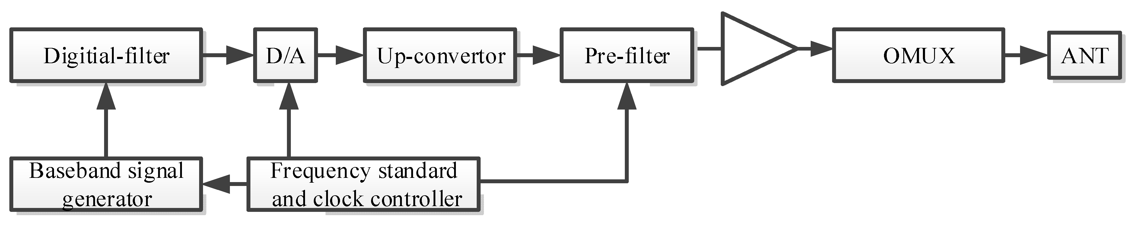
2.1. Navigation Payload Model

As shown in Figure 1, the navigation signal generating unit completes the modulation of the spreading code, subcarrier, and data message to obtain an ideal infinite bandwidth constant envelope baseband signal. Next, the harmonics and mirror signal interference are filtered out for digital-to-analog conversion. Afterward, the out-of-band spurious and harmonic interference are filtered and then upconverted to the broadcast frequency. Through HPA amplification, it enters the multiplexer for signal multiplexing. Finally, it is broadcast by the antenna.

As shown in Figure 1, the navigation payload transmission channel is mainly composed of digital and analog components, and each component has different effects on the signal quality [9,10,11,12,13,14,15]. The baseband signal generation and digital filtering usually introduce small linear distortion. D/A conversion and up-conversion are usually modeled as linear distortions because of the same source as baseband signal frequency synthesis [15]. Pre-band-limit filtering destroys the constant envelope characteristics of the signal, resulting in severe nonlinear distortion after HPA [15]. After output filtering and multiplexing, this becomes even worse. The navigation signal is an intuitive reflection of the characteristics of the transmission channel. Comparing the influence of different units on the signal, as shown in Figure 2, this work models the navigation payload signal distortion in equivalently two parts: digital distortion and analog distortion [10]. In this work, the influence before HPA is uniformly classified as digital distortion, whereby it is considered that digital devices only bring a time delay and do not affect signal waveform distortion. Hence, the digital distortion is represented using the classic TMA model, and the analog distortion acts on the digital distortion totally. The analog distortion is equivalently modeled as an N-order FIR filter due to the limited-band pre-filter of HPA. The amplitude and group delay are used to characterize the filter characteristics. The specific mathematical derivation is provided below.

The ideal multiplexed signal is

$$s(t)={\displaystyle \sum _{n=1}^N{A}_n}{\mathrm{e}}^{j{\theta }_n}{s}_n(t)+IM(t),$$

(1)

where $s_n(t)$ is the ideal single-branch binary signal, $A_n$ is the amplitude, ${\theta }_n$ is the phase, and $IM(t)$ is the intermodulation term. It is defined that the digital distortions between each branch are independent and band-unlimited, and the multiplexed signal can be rewritten as

$$x(t)={\displaystyle \sum _{n=1}^N{A}_n}{\mathrm{e}}^{j{\theta }_n}{s}^{△}{}_n(t)+IM(t),$$

(2)

where $\Delta =\eta T_c$ is the digital distortion, $\eta \in (-1,1)$, and $T_c$ is the spreading code rate. In other words, the digital distortion will not exceed one chip.

Analog distortion is introduced on the basis of digital distortion. In this work, the analog distortion is modeled as an N-order linear FIR filter; hence, the signal is the convolution of the input signal and the analog impulse response.

$$y(t)=x(t)\otimes h(t),$$

(3)

where $h(t)$ is the impulse response of the filter, and $\otimes$ represents the convolution calculation.

Assuming that all branches can be completely separated, after analog distortion, the single branch signal is

$${\tilde{s}}_n(t)=s^{△}{}_n(t)\otimes h(t).$$

(4)

Correspondingly, the correlation with the local ideal signal is

$$\begin{array}{l}{\widehat{R}}_n(\tau )=\frac{1}{T_p}{\int }_{T_p}{\tilde{s}}_n(t)s_n^{*}(t-\tau )dt\\ ={\tilde{s}}_n(\tau )\otimes s_n^{*}(\tau )\otimes h(\tau )=R_n(\tau )\otimes h(\tau ),\end{array}$$

(5)

where $T_p$ indicates the period (or code epoch duration) of the signal components, $R_n(\tau )$ represents the autocorrelation function of the $n\mathrm{th}$ branch, and $*$ is a conjugate matrix.

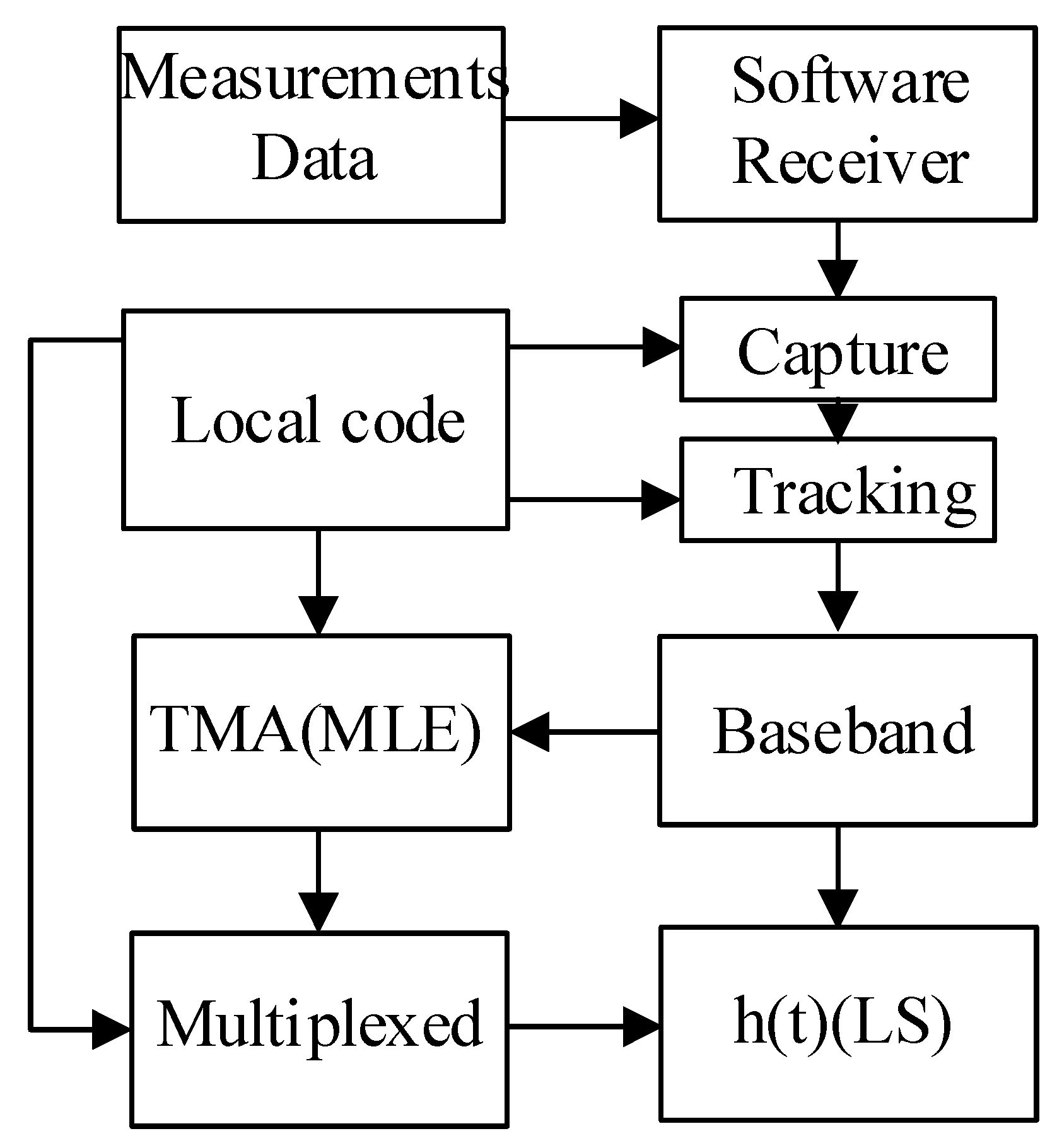
2.2. Joint Estimation Algorithm

The continuous baseband signal is obtained after preprocessing by the software receiver. Accumulating and averaging continuous baseband signals can effectively reduce noise interference [14]. The baseband signal $y$ after processing is recorded as

$$y={\left[y_1,y_2,\dots ,y_p\right]}^T,$$

(6)

$$h={\left[h_1,h_2,\dots ,h_m\right]}^T,$$

(7)

where $p$ is the sampling point, $h$ is the analog impulse response matrix, and $m$ is the order of the filter. The digital distortion of the single-branch signal is

$$\eta ={\left[{\eta }_1,{\eta }_2,\dots ,{\eta }_N\right]}^{\mathrm{T}}{\eta }_n\in (-1,1),$$

(8)

where

$N$ indicates the number of branches, and $\eta$ is the digital distortion matrix. Thus, the $n\mathrm{th}$ signal is

$$x_{{\eta }_n}={[x_{{\eta }_n}(1),x_{{\eta }_n}(2),\dots ,x_{{\eta }_n}(p)]}^T.$$

(9)

$X({\eta }_n)$ can be denoted as the $n\mathrm{th}$ branch signal convolution matrix.

$$X({\eta }_n)={\left[\begin{array}{cccc}{x}_{{\eta }_n}(1)& x_{{\eta }_n}(p)& \dots & x_{{\eta }_n}(p-m+2)\\ x_{{\eta }_n}(2)& x_{{\eta }_n}(1)& \dots & x_{{\eta }_n}(m+1)\\ \dots & \dots & \dots & \dots \\ x_{{\eta }_n}(p)& x_{{\eta }_n}(p-1)& \dots & x_{{\eta }_n}(p-m+1)\end{array}\right]}^T.$$

(10)

The navigation payload transmission channel characteristic can be transformed into a maximum likelihood estimation (MLE) joint estimate for the digital distortions and analog impulse response [10].

$$(\tilde{\eta },\tilde{h})=\underset{\eta ,h}{\arg \max }\left\{\Vert y-X(\eta )h{\Vert }_2^2\right\},$$

(11)

where $X(\eta )$ indicates the multiplexed signal convolution matrix, and $\tilde{\eta }$ indicates the digital distortion estimation matrix.

Furthermore, the $n\mathrm{th}$ branch digital distortion ${\tilde{\eta }}_n$ is an analytical equation describing the measurement signal and the input convolution matrix.

$${\tilde{\eta }}_n=\underset{{\eta }_n}{\arg \max }\{y^{\mathrm{H}}X({\eta }_n){(X{({\eta }_n)}^{\mathrm{H}}X({\eta }_n))}^{-1}X{({\eta }_n)}^{\mathrm{H}}y\}.$$

(12)

Different input signal matrices can be obtained by traversing ${\tilde{\eta }}_n$; the maximum value calculated by Equation (12) is the optimal ${\tilde{\eta }}_n$ under the maximum likelihood probability. The optimal ${\tilde{\eta }}_n$ of each branch can be calculated using the above method, and a new multiplexed signal can be synthesize. At this time, the new multiplexed signal matrix $X(\eta )$ contains digital distortion. Thus, an estimate of the simulated analog impulse response can be easily obtained from the least squares (LS) method.

$$\tilde{h}={(X{(\eta )}^{\mathrm{H}}X(\eta ))}^{-1}X{(\eta )}^{\mathrm{H}}y,$$

(13)

where $\mathrm{H}$ represents transpose, and $\tilde{h}$ is the analog impulse response estimation matrix.

So far, the digital distortion and analog impulse responses of the navigation payload transmission channel have been estimated, with no overly complicated calculation. The algorithm structure corresponding to the above theoretical derivation is shown in Figure 3.

Firstly, the software receiver is used to preprocess the large antenna measurement data to obtain the initial baseband signal. The MLE is then used to obtain the digital distortion for each branch. Next, a new multiplexed signal is synthesized using the digital distortion of each branch. Finally, the impulse response of the analog channel is obtained using the LS method. In the whole process, the software receiver part can use different classical algorithms according to the requirements.

3. Results Analysis

3.1. Measurements with NTSC’s High-Gain Antenna

The NTSC of the Chinese Academy of Sciences operates a GNSS space signal quality assessment system with a 40 m large-diameter antenna as the core. The antenna L-band gain is greater than 50 dBi, the beam width is about 0.3°, and the tracking accuracy of the antenna is about 0.015° [16]. The signal received by the large-diameter antenna is transmitted to the computer room through the optical fiber [16]. The ground receiving station is also equipped with an accurate channel calibration subsystem to minimize the impact on signal quality. The parameters of the system can be found in [17]. The signal received by the large-diameter high-gain antenna is considered to be unaffected by multipath interference, and the software receiver can accurately estimate and eliminate the Doppler effects. The classical parallel frequency search method and bump-jump technique are used for code-phase and carrier frequency tracking [18]. Meanwhile, the following conditions are assumed to hold:

• The in-phase and quadrature (I/Q) branch is completely separated, and the related outputs are irrelevant;
• The mixed effect of signal distortion and external noise will not lead to loss of lock, and the tracking jitter is negligible;
• In a short time, the influence of the spatial transport layer is ignored in a small area.

Under the above assumptions, the actual received signal is considered to be very close to the navigation payload transmitted signal.

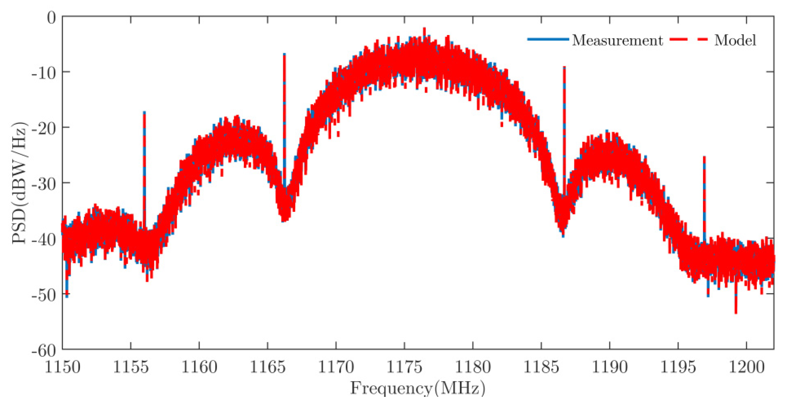
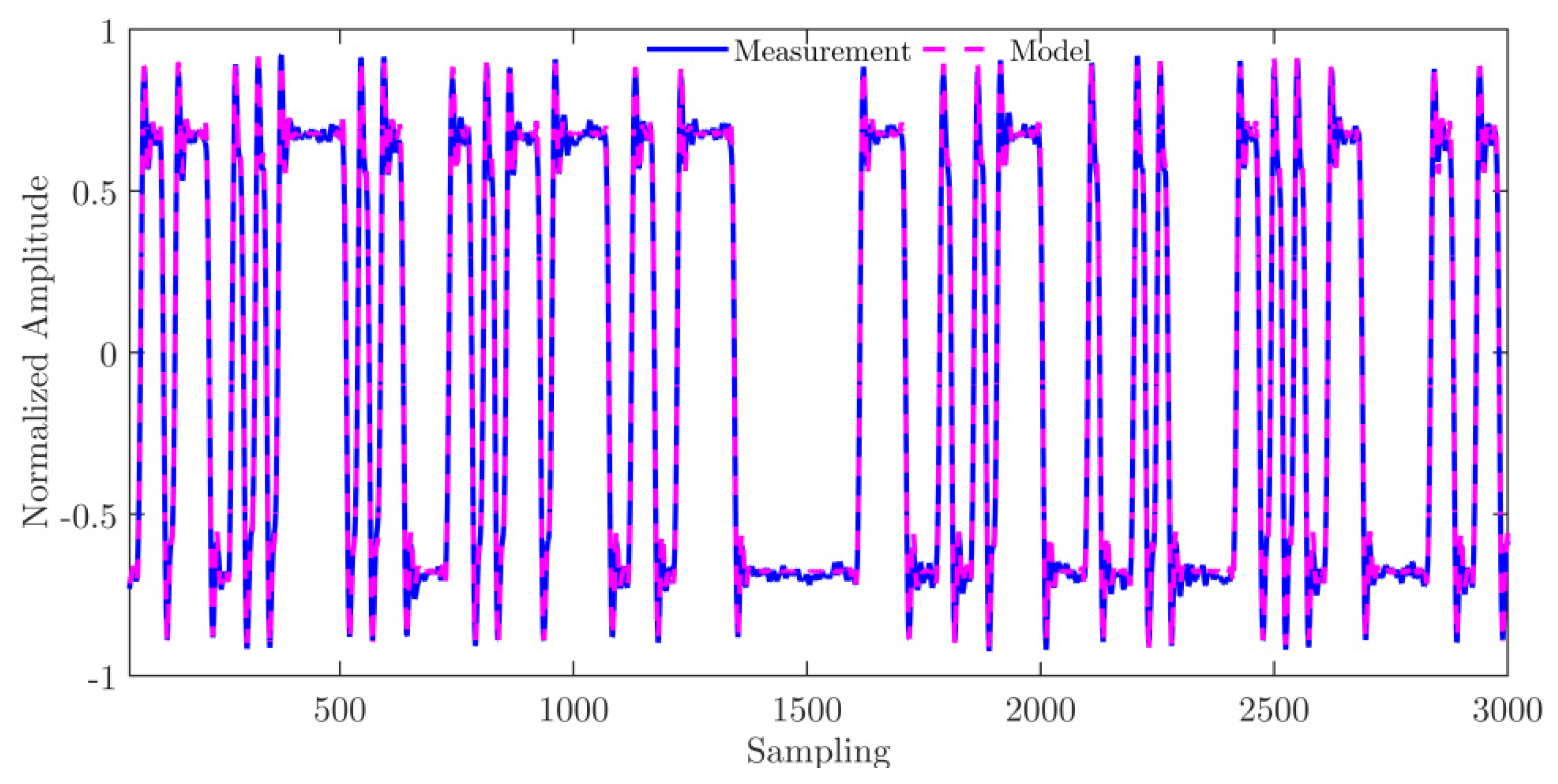
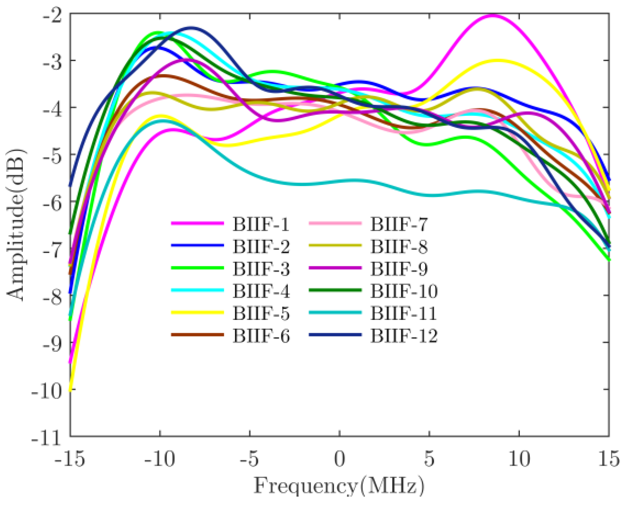
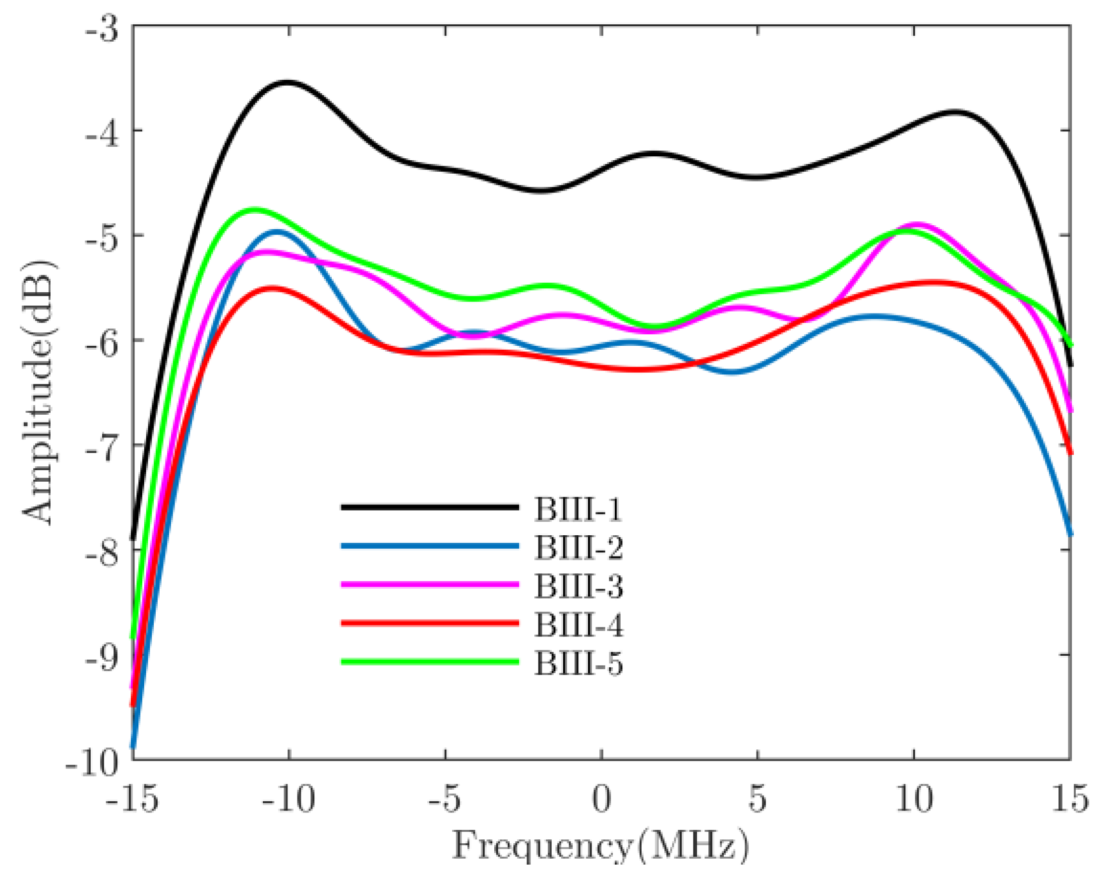
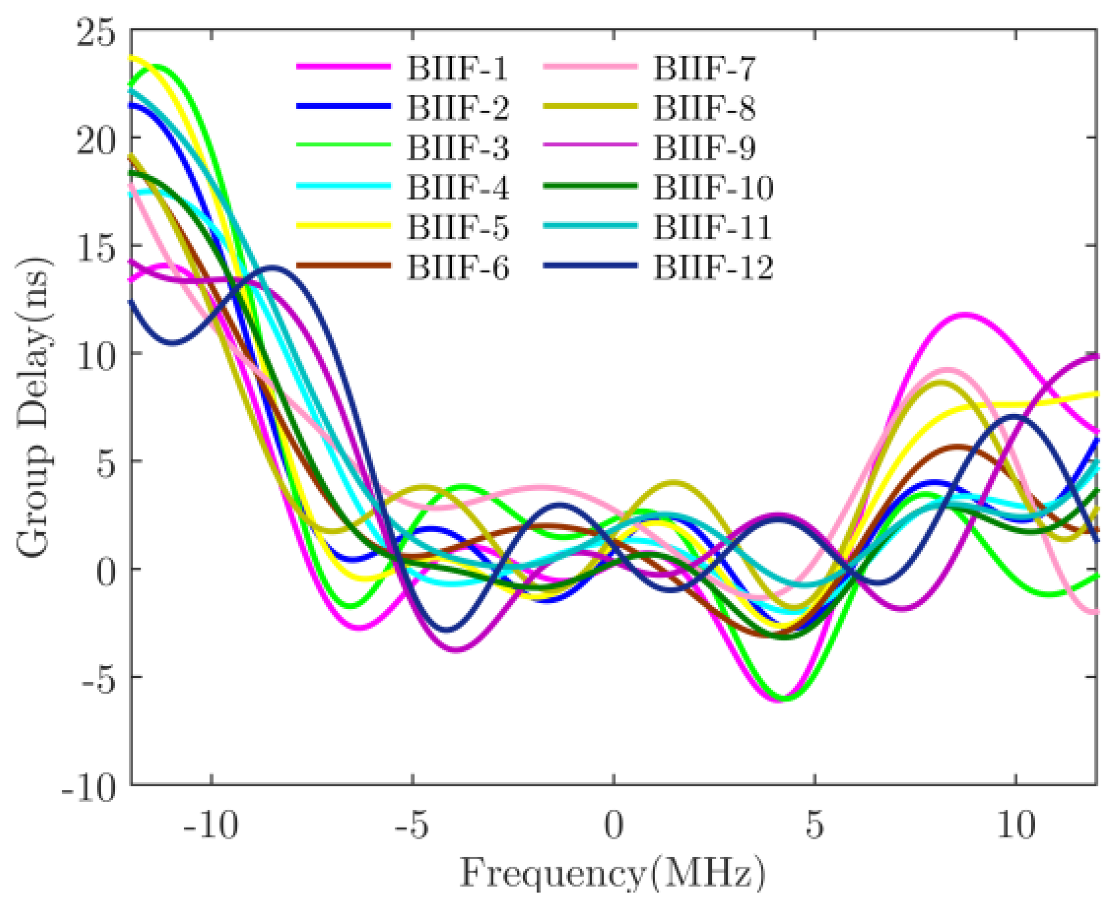
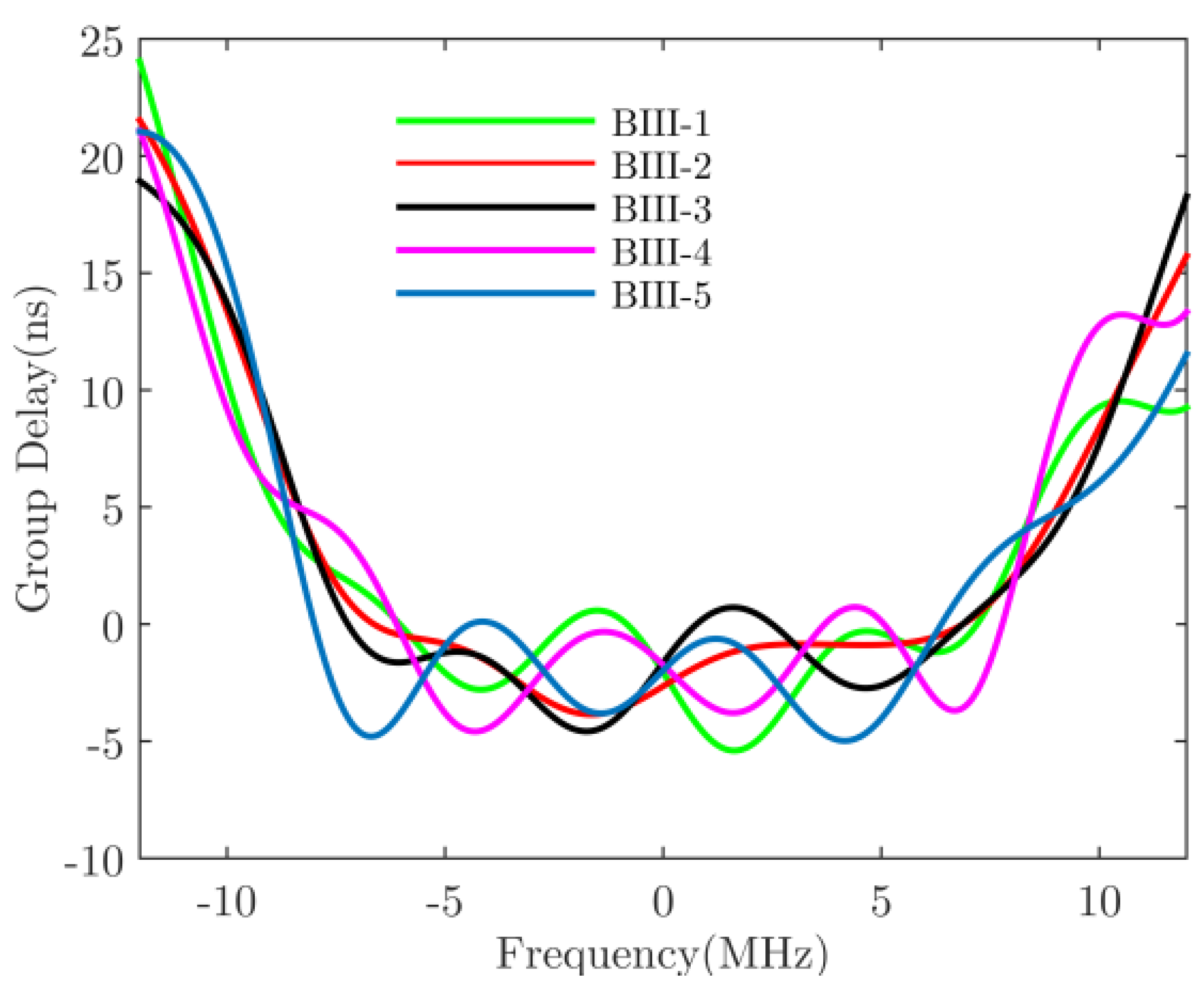
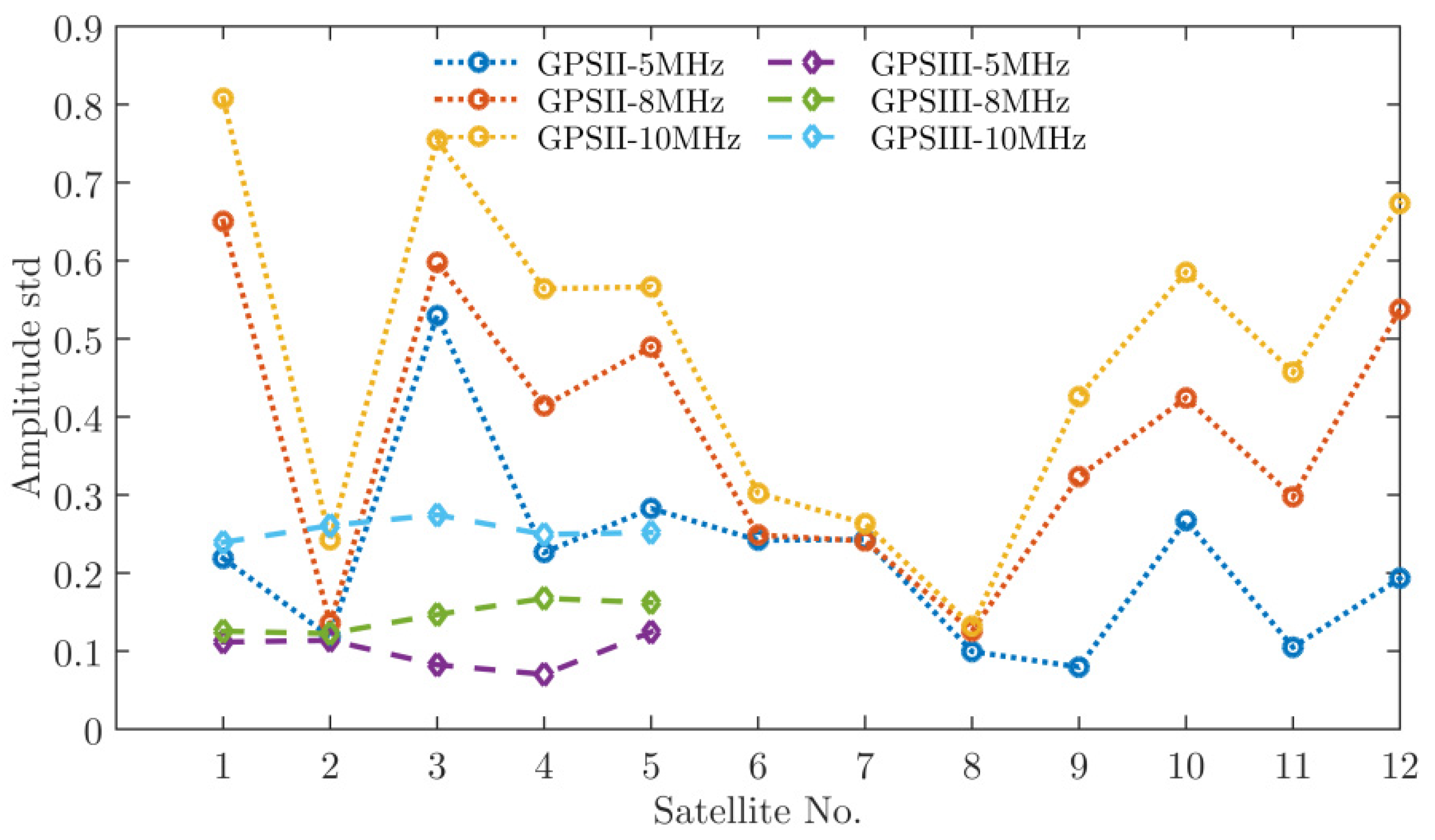
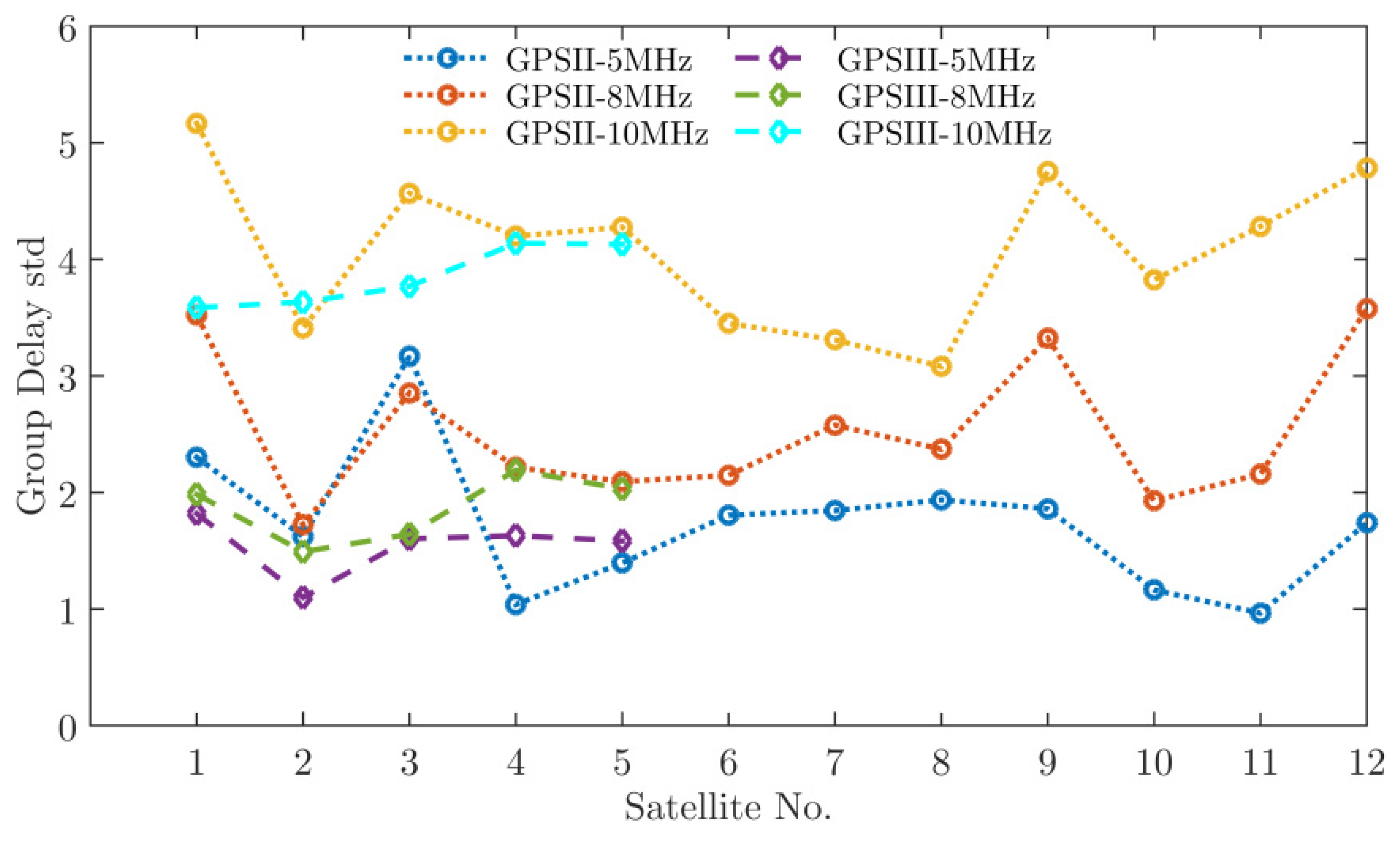
3.2. Signal Analysis

This section first verifies the feasibility and accuracy of the model and algorithm from the time-domain waveform and the power spectrum density (PSD). On this basis, the digital and analog impulse responses of GPS II and GPS III signals are estimated and analyzed in detail. Finally, the ranging error reference of the signal under the estimated navigation payload transmission channel is given to the user receivers.

Measurements of all GPS BIIF and GPS III satellites were performed with NTSC’s 40 m high-gain antenna at the ground station of Hao-ping, to serve as data for analysis of signal distortion. The signal sampling rate was set to 250 MHz, and the accumulated average was 100 code periods. To verify the accuracy of the model and estimation algorithm, this study first compares the differences between the measured data and model calculations from power spectra and time-domain waveforms.

BIIF-5 and BIII-2 are considered as examples of GPS II and GPS III, respectively. Figure 4, Figure 5, Figure 6 and Figure 7 compare the measured signal and model estimation results from the time and frequency domains, respectively. Regardless of it being a GPS II or a GPS III signal, the figure indicates that the power spectrum and the time-domain waveform estimated by the model are completely consistent with the measured signal. The above results directly demonstrate the effectiveness and accuracy of the models and algorithms in this work. A significant carrier leakage due to digital distortion can be observed at integer multiples of the power spectrum in Figure 5, which was present in all BIIF satellites. However, referring to Figure 7, this phenomenon was absent in GPS III satellites. From the power spectrum, it is evident that the digital distortion of the GPS III satellite transmission channel was significantly improved. The digital distortion was further calculated according to the joint estimation method.

Table 1. Navigation payload transmission channel digital distortion.

Satellite	BIIF-1	BIIF-2	BIIF-3	BIIF-4	BIIF-5	BIIF-6	BIIF-7	BIIF-8	BIIF-9	BIIF-10	BIIF-11	BIIF-12	GPS III-1	GPS III-2	GPS III-3	GPS III-4	GPS III-5
Data (%)	−3.2	−2.1	−3.0	−2.0	−3.0	−3.0	−2.0	−2.0	−1.0	−2.0	−1.0	−2.0	0.0	0.0	0.0	0.0	0.0
Pilot (%)	−1.1	−2.0	−2.0	−2.0	−5.0	−6.0	−5.0	−4.0	−2.0	−1.0	−4.0	−3.0	0.0	0.0	0.0	0.0	0.0

summarizes the L5 digital distortion for the latest data from all launched GPS IIF and GPS III satellites.

It can be seen from Table 1 that all BIIF satellites had different degrees of digital distortion. The BIIF-1 satellite had the highest digital distortion of the L5 data signal, reaching 3.2% chips; BIIF-9 and BIIF-11 satellites had the lowest at 1% chips. For the L5 pilot signal, digital distortion in the BIIF-6 satellite was the highest, reaching 6% chips, whereas that in the BIIF-10 satellite was the smallest, at 1% chips. In addition, the BIIF-1, BIIF-3, and BIIF-5–12 satellites had inconsistent digital distortions of data and the pilot signal, with a maximum difference of 3% chips. Data and pilot inconsistencies indicate an imbalance in the quadrature modulation I/Q branch. Although the digital distortion of GPS II was small and tolerable, GPS III had negligible digital distortion compared with GPS II, consistent with the PSD. After the digital distortion was calculated accurately, the satellite analog impulse response could be estimated. Figure 8, Figure 9, Figure 10 and Figure 11 show the amplitude and group delay characteristics of the navigation payload analog channel.

Ideally, the analog channel amplitude and group delay should be constants within the main lobe bandwidth. However, there were different degrees of jitter in the group delay and amplitude affected by the analog device. It can be seen from the figure that, in terms of amplitude and group delay characteristics, the consistency of the analog channel in GPS III satellites was better than that in GPS II satellites. To further analyze the details, the standard deviations of the amplitude and group delay within different bandwidths were considered.

It can be seen from Figure 12 that, under different bandwidths, the amplitude standard deviations of BIII were better than those of BIIF. In the 5 MHz bandwidth, the amplitude standard deviations of BIII satellites were approximately 0.1, whereas those of the BIIF satellites fluctuated between 0.1 and 0.55. In the 8 MHz bandwidth, the amplitude standard deviation of the BIII satellite was in the interval 0.13–0.16, whereas, for BIIF, the interval was 0.13–0.65 under the same conditions. In the 10 MHz bandwidth, the amplitude standard deviations of BIII were approximately 0.25, whereas, for BIIF satellites, they fluctuated between 0.13 and 0.80. Similarly, Figure 13 describes the standard deviations of group delay in different bandwidths.

As indicated by Figure 13, unlike the amplitude characteristics, the standard deviations of the group delay presented a more complex characteristic. In the 5 MHz bandwidth, the group delay standard deviations of the BIII satellites were in the interval 1.0–1.8, whereas, for BIIF satellites, they fluctuated between 0.9 and 2.3. In the 8 MHz bandwidth, the group delay standard deviations of the BIII satellite were in the interval 1.4–2.2, whereas, for BIIF, they ranged between 1.7 and 3.5. In the 10 MHz bandwidth, the amplitude standard deviations of the BIII and BIIF satellites were in the intervals 3.5–4.2 and 3.0–5.4, respectively. According to the above analysis of the amplitude and group delay, it is evident that the analog channel was more strongly affected by the group delay. Additionally, the navigation payload transmission channel performance of the GPS III system L5 signal was improved, as compared with that of GPS II, regardless of the amplitude or the group delay characteristics.

The S-curve bias (SCB) is an index for evaluating the ranging bias of navigation signals [11]. Ideally, the navigation payload transmission channel SCB should be 0. However, the navigation payload transmission channel was affected by various digital and analog devices, which inevitably introduced ranging errors. In addition, the ranging deviations in satellites were different due to the analog devices used, and this error could not be deducted by differentiation. According to the above estimated digital and analog distortions, this study provides a ranging error reference for user receivers. For subsequent analyses, the receiver unilateral bandwidth setting range was 6–12 MHz, the correlator interval was within 0.5 chips, and the absolute maximum value of SCB was considered, as shown in

Table 2. Maximum SCB range.

Satellite	BIIF-1	BIIF-2	BIIF-3	BIIF-4	BIIF-5	BIIF-6	BIIF-7	BIIF-8	BIIF-9	BIIF-10	BIIF-11	BIIF-12	GPS III-1	GPS III-2	GPS III-3	GPS III-4	GPS III-5
Data (m)	0.032	0.032	0.034	0.032	0.032	0.027	0.031	0.028	0.031	0.031	0.032	0.031	0.016	0.013	0.010	0.011	0.009
Pilot (m)	0.032	0.030	0.030	0.032	0.031	0.030	0.031	0.032	0.031	0.032	0.031	0.031	0.019	0.010	0.014	0.012	0.010

. Figure 14 and Figure 15 show the SCBs for BIIF and GPS BIII for different user receiver settings, respectively.

Table 2 shows the statistical results of SCB for all satellites. As shown in the table, the SCB of the GPS II signal fluctuated in the range 0.027–0.034 m. By contrast, the SCB of the GPS III signal was concentrated at 0.01 m, indicating that the ranging bias was improved by approximately 0.02 m. Therefore, the user positioning accuracy can be effectively improved by estimating the transmission channel of the navigation payload and providing the user with the resulting ranging deviation.

4. Discussion

The first GPS III satellite was launched in December 2018, and five satellites have been launched so far. As the third important stage of GPS modernization, the GPS III signal has significantly improved. According to the performance of each component of the navigation payload transmission channel, unlike previous estimations of the channel, digital distortion was considered in signal distortion modeling in this paper. The accuracy of the signal distortion model and estimation method was verified on the basis of the measurement data of a large-aperture antenna, and the GPS II and GPS III L5 transmission channels and the resulting ranging biases were compared for the first time. However, the following aspects still need to be further explored in follow-up research: the consistency of I/Q branch modulation methods of the GPS L5 signal; signals of different modulation methods, such as the GPS L1 signal.

5. Conclusions

Through the long-term monitoring and evaluation of GPS signals, it was observed that GPS III signals improved significantly as compared to GPS II signals. This work established a signal distortion model according to the characteristics of the navigation load components. Furthermore, all GPS satellite digital distortions and analog impulse responses were estimated simultaneously using the joint estimation method. The analysis revealed that, compared with those of GPS II, the digital distortions of GPS III were negligible. With regard to the analog impulse response, GPS III satellites exhibited better amplitude and group delay consistency than GPS II. Lastly, the ranging bias caused by the navigation payload channel improved by approximately 0.02 m in GPS III satellites, as compared with that of GPS II satellites.

References

1. He, C.Y.; Guo, J.; Lu, X.C. A new evil waveform evaluating method for new BDS navigation signals. GPS Solut. 2018, 22, 37–50. [Google Scholar] [CrossRef]
2. BeiDou Navigation Satellite System Signal in Space Interface Control Document, Open Service Signal B1I (Version 3.0). China Satellite Navigation Office, February 2019. Available online: http://www.beidou.gov.cn (accessed on 21 August 2020).
3. European GNSS (Galileo). Open Service Signal in Space Interface Control Document; European Union and European Space Agency: Paris, France, November 2015; Issue 1.2; Available online: https://galileognss.eu (accessed on 18 August 2020).
4. GPS Global Positioning System Directorate Systems Engineering and Integration. IS-GPS-200J NAVSTAR GPS Space-Segment/Navigation User Segment Interfaces. 22 May 2018. Available online: https://www.gps.gov (accessed on 6 April 2022).
5. Li, C.H.; Liu, Y.X.; Mo, W.H.; Ou, G. Analysis of the impact of satellite’s high power amplifier on the performance of navigation signals carrier tracking. J. Natl. Univ. Def. Technol. 2013, 35, 81–84. [Google Scholar]
6. Chen, Y.B.; Kou, Y.H.; Zhang, Z.W. Analog distortion of wideband signal in satellite navigation payload. In Proceedings of the China Satellite Navigation Conference (CSNC), Guangzhou, China, 15–19 May 2012; pp. 89–100. [Google Scholar]
7. Yu, X.L.; Kou, Y.H. Simulation of analog distortion of dual-frequency multiplexing signal generated by navigation satellite. J. Beijing Univ. Aeronaut. Astronaut. 2018, 44, 1048–1055. [Google Scholar]
8. Liu, Y.Q.; Chen, L.; Yang, Y.; Pan, H.; Ran, Y.H. Theoretical evaluation of group delay on pseudo range bias. GPS Solut. 2019, 23, 69–71. [Google Scholar] [CrossRef]
9. Rebeyrol, E.; Macabiau, C.; Julien., O.; Issler., J.L. Signal distortions at GNSS payload level. In Proceedings of the International Technical Meeting of the Satellite Division of The Institute of Navigation (ION GNSS 2006), Fort Worth, TX, USA, 26–29 September 2006; pp. 1595–1605. [Google Scholar]
10. Thoelert, S.; Vergara, M.; Sgammini, M.; Enneking, C.; Antreich, F.; Meurer, M.; Brocard, D.; Rodrigues, C. Characterization of Nominal Signal Distortions and Impact on Receiver Performance for GPS (IIF) L5 and Galileo (IOV) E1/E5a Signals. In Proceedings of the 27th ION National Technical Meeting, Tampa, FL, USA, 9–12 September 2014. [Google Scholar]
11. Kou, Y.; Wu, H. Model and implementation of pseudo-range bias free linear channel. GPS Solut. 2021, 25, 53. [Google Scholar] [CrossRef]
12. Phelts, R.E.; Akos, D. Effects of signal deformations on modernized gnss signals. J. Glob. Position. Syst. 2006, 5, 2–10. [Google Scholar] [CrossRef] [Green Version]
13. Yan, T.; Wang, Y.; Qu, B.; Liu, X. Analysis Methods of Linear Distortion Characteristics for GNSS Signals. In Proceedings of the China Satellite Navigation Conference (CSNC) 2018, Harbin, China, 23–25 May 2018; pp. 183–195. [Google Scholar]
14. Kang, L.; Lu, X.; Wang, X.; He, C.; Rao, Y. Navigation Signal Chip Domain Assessment on Beidou Navigation System. J. Electron. Inf. Technol. 2018, 40, 1002–1006. [Google Scholar] [CrossRef]
15. Wang, Y.; Yan, T.; Wang, G.; Bian, L.; Meng, Y. Analysis of Interaction between Navigation Payload and Constant Envelope Design of Navigation Signal. In Proceedings of the China Satellite Navigation Conference (CSNC) 2019, Beijing, China, 25–28 May 2019; pp. 421–431. [Google Scholar]
16. Shi, H.H.; Wang, M.; Rao, Y.; Lu, X.; Wang, X. Researches on Pro-retirement Signal Quality of BeiDou Navigation Satellite System GEO-3 Satellite B1 Signal. J. Electron. Inf. Technol. 2020, 42, 1573–1580. [Google Scholar] [CrossRef]
17. Lu, X.; He, C.; Wang, X. Design of GNSS Monitoring and Assessment System and Assessment of GNSS Signal-in-Space. J. Time Freq. 2016, 39, 225–246. [Google Scholar] [CrossRef]
18. Kaplan, E.D.; Hegarty, C.J. Understanding GPS Principles and Applications, 3rd ed.; Artech House: Norwood, MA, USA, 2018. [Google Scholar]
Figure 1. Navigation payload transmission channel model.
Applsci 12 03791 g001
Figure 2. Signal distortion model on navigation payload.
Applsci 12 03791 g002
Figure 3. Joint estimation algorithm block.
Applsci 12 03791 g003
Figure 4. BIIF-5 L5-Cd time-domain waveform.
Applsci 12 03791 g004
Figure 5. BIIF-5 L5 PSD.
Applsci 12 03791 g005
Figure 6. BIII-2 L5-Cd time-domain waveform.
Applsci 12 03791 g006
Figure 7. BIII-2 L5 PSD.
Applsci 12 03791 g007
Figure 8. BIIF-5 amplitude characteristic.
Applsci 12 03791 g008
Figure 9. BIII-2 amplitude characteristic.
Applsci 12 03791 g009
Figure 10. BIIF-5 group delay characteristic.
Applsci 12 03791 g010
Figure 11. BIII-2 group delay characteristic.
Applsci 12 03791 g011
Figure 12. Standard deviations of amplitude under different bandwidths.
Applsci 12 03791 g012
Figure 13. Standard deviations of group delay under different bandwidths.
Applsci 12 03791 g013
Figure 14. BIIF-5 L5-Cd SCB.
Applsci 12 03791 g014
Figure 15. BIII-2 L5-Cd SCB.
Applsci 12 03791 g015