Abstract
Deep neural network models have been developed in different fields, bringing many advances in several tasks. However, they have also started to be incorporated into tasks with critical risks. That worries researchers who have been interested in studying possible attacks on these models, discovering a long list of threats from which every model should be defended. The weight modification attack is presented and discussed among researchers, who have presented several versions and analyses about such a threat. It focuses on detecting multiple vulnerable weights to modify, misclassifying the desired input data. Therefore, analysis of the different approaches to this attack helps understand how to defend against such a vulnerability. This work presents a new version of the weight modification attack. Our approach is based on three processes: input data clusterization, weight selection, and modification of the weights. Data clusterization allows a directed attack to a selected class. Weight selection uses the gradient given by the input data to identify the most-vulnerable parameters. The modifications are incorporated in each step via limited noise. Finally, this paper shows how this new version of fault injection attack is capable of misclassifying the desired cluster completely, converting the 100% accuracy of the targeted cluster to 0–2.7% accuracy, while the rest of the data continues being well-classified. Therefore, it demonstrates that this attack is a real threat to neural networks.
1. Introduction
Nowadays, computational power has allowed the development of new architectures in the growing field of deep learning. In some tasks, they can outperform human beings in their remits, and hence, these networks are being implemented in more and more fields with a direct impact on the lives of human beings [1,2]. In addition, models used in some fields such as healthcare or autonomous vehicles have to make critical decisions affecting human lives. These models can be compromised, putting lives at risk. For these two reasons, in recent years, research has been carried out on how a model can be attacked and defended to make neural networks more secure and reliable.
Several state-of-the-art attacks on neural networks have been proposed [3,4,5]. A machine learning system (Figure 1) can be separated into several elements: training data, input data, model, and prediction (output). The attacks found in the literature can be grouped into these elements according to their focus.
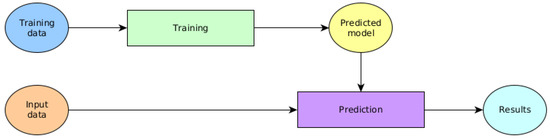
Figure 1.
Schematic representation of a machine learning system.
- Training data attacks: Attacks that threaten the training data are those that exploit the modification of this data to attack the target model. Thus, the attacker causes a malfunction modifying its proper behavior. Among the attacks focused on this module are the poisoning attack [6,7] and the obfuscation attack [8].
- Input data module: Attacks to the input data are implemented to somehow affect the predicted output of the model. The attacker studies samples to corrupt the behavior of the target model. In this category, we would find the widely known adversarial attack. Moreover, this element contains other attacks, such as the overstimulation attack [9], the evasion attack [10], the impersonation attack [11], and the feature deletion attack [12].
- Prediction attacks: Predictions can also provide valuable information about the inner structure of the model to the adversary. The model shows different behaviors depending on the input received, which can reveal sensitive or private information contained in the model. Therefore, in this module, we can find privacy attacks such as the inversion attack [13], the inference attack [14], and the Ateniese attack [15].
- Model element: Other attacks focus on attacking the model directly. These attacks can modify parameter values, model structures or model functions. Attacks directed against this module are those related to obtaining parameters and hyperparameters, such as the equation-solving attack [16] and hyperparameter stealing [17]. However, in many cases it is also possible to attack model parameters by directly modifying their values. This is the case of the fault injection attack described by Liu et al. [18].
In the evasion attack [10], the adversary directly modifies the input sample to obtain a misclassified instance. However, that modification tends to be passed over due to the input weights of the target model, bypassing the malicious data. In this case, the manipulation converts the target data into misclassified data without modifying it. There are a lot of adversarial attacks affecting the input of a model, but in actual deployments, it can be easier for a potential intruder to change the model’s available inputs. Therefore, in this sense, an attack that modifies the model parameters is more general than an evasion attack because the evasion attack obtains a single malicious sample, while the described attack converts complete subsets of target input data into misclassified data. However, parameter manipulation can also change the prediction of the data that the attacker does not want to change. Therefore, an exhaustive analysis of the selection of the weights to be manipulated is necessary.
In this work, a new approach to the fault injection attack is presented. This version incorporates three steps to attack the targeted model, making the manipulation more efficient.
- Identifying input data clusters: Similar input data generates similar model behaviors given by the activation of the model’s neurons. Therefore, they could share influential weights, which would not be applicable for the other data. Thus, modification of these parameters will affect the targeted cluster.
- Selection of the most-influential weights: This step chooses some weights to be modified. For this selection, a metric is necessary; some types of adversarial attacks target the gradient of the input data according to the prediction. Thus, the idea is based on introducing a constant adversarial example in the model for a concrete input data subset.
- Modification of the selected weights: Incorporation of noise in the chosen weights is essential to manipulate the prediction of the targeted model. Noise can be added or subtracted according to the computed gradient, modifying the behavior differently. This decision allows the attacker to focus on varying weights.
This new version allows more precise manipulation and without misclassifying the non-targeted input data. This attack was tested with a model formed by the convolutional neural network VGG16 and a dense classifier, which deals with a binary classification problem.
The rest of the paper is divided as follows: Section 2 presents the literature related to the analyzed attack. Section 3 details the attack generation, highlighting the principal steps to carry out the attack. Section 4 describes the experiments detailing the dataset and the model used for them. The results are given in Section 5, and Section 6 lists the lessons learned and future work.
2. Background
Model parameter modification attack was introduced first by Liu et al. [18] and named fault injection attack. They proposed two attack strategies: one by only modifying the bias values of the model, single-bias attack (SBA), and the other, gradient descent attack (GDA), that pursued maintaining model accuracy by mitigating the impact of other input patterns and centering modified weights in a specific layer. In SBA, the proposed bias modification is independent of the input value, i.e., it only depends on the sensitivity of the bias to the selected class. That allows applying the attack in real-time without analyzing the input data characteristics. The GDA attack is centered on modifying a single input data prediction. Furthermore, the level of modification of the weights is uniquely dependent on the number of neurons in the selected layer, as they directly use the gradient descent algorithm to modify them at once.
Zhao et al. [19] detailed the theoretical problem formulation and applied it to fully connected neural networks, modifying the bias and weight parameters. Their results showed that it is possible to attack the models by this strategy while controlling the damage to model accuracy. Their novel solution allows attacking multiple images with a unique attack. Moreover, it uses the ADMM framework for dividing the global problem into more minor local issues. However, the particular similarities between the selected images are not analyzed to guide the optimization problem directly, centering the modification on the most influential parameters.
Rankin et al. [20] demonstrated how to achieve targeted adversarial attacks by modifying the weights by flipping the smallest possible number of bits of weight values. They propose an iterative process, where in each iteration, a single weight-bit is selected and flipped. For its selection, an intra-layer bit search is first applied in each iteration, selecting the most vulnerable weight-bit in each layer using gradient values. Then, a cross-layer search is pursued from the selected subset of bits, identifying the layer with maximum loss due to bit-flip. The winner-layer weight-bit is the only bit chosen to be flipped in the iteration.
The sensitivity of the model to this attack was also studied. On the one hand, Tsai et al. [21] described the generalization of the weight perturbation sensitivity for feed-forward neural networks and described the robustness of the models to this attack category. From their perspective, the sensitivity of the weight is related to the pairwise class margin function against weight perturbation. On the other hand, Weng et al. [22] specifically studied the robustness of the model in response to model weight perturbations attacks. For that purpose, for each weight value, they define regions near the specific value where the model can maintain accuracy. Taking into account the sizes of these regions, a model robustness measure can be defined against this type of attack.
Finally, new defenses are emerging to avoid fault injection attacks. Wang et al. [23] propose a defense against this type of attack, increasing the robustness of the model using a novel randomization scheme called hierarchical random switching (HRS). This defense contains multiple channels in the model with different weight values that a controller switches, making this type of attack unfeasible. The advantage of this defense compared to ensemble defenses that use multiple networks is that HRS only requires a single base network architecture to launch the defense.
The references detailed above are related to the presented version of the fault injection attack, but comparison with the actual proposal is complicated since they share a unique step in attack generation. Furthermore, some of the cited background strategies are not even formulated as attacks. With this in mind, the most-similar reference is [18], which presents an attack strategy that searches for the most-sensitive parameters through use of the gradient. However, the gradient they use is over the weights and not over the input features, as the version proposed in this paper is. Moreover, ref. [18] does not use the clusterization step to optimize the attack; rather, it selects a sample subset randomly. In [19,20], they present attack versions which focus on the whole targeted model, and they use neither the gradient nor clusterization. Finally, refs. [22,23] describe strategies related to the search of vulnerability parameters, similar to our version, but they are not presented as an attack. On the one hand, ref. [22] details a possible method of clusterization of the input data, focusing on the model’s prediction, while our strategy focuses on the input features for that objective. On the other hand, ref. [23] presents a methodology to detect the vulnerable weights by injecting noise in the target model instead of using the gradient as the weight metric.
3. Methodology
This work aims to implement a weight modification attack with an optimized search of the most-influential parameters for attacking the desired samples (Figure 2). The main idea of the attack is to modify a minimal quantity of weights from the target model to obtain misclassification of the targeted input data. Concretely, this approach attacks a particular layer of the targeted model. Take into account that the targeted layer’s input features will be considered as the input data, and the input layer will be the neurons that introduce the input data to the target layer.
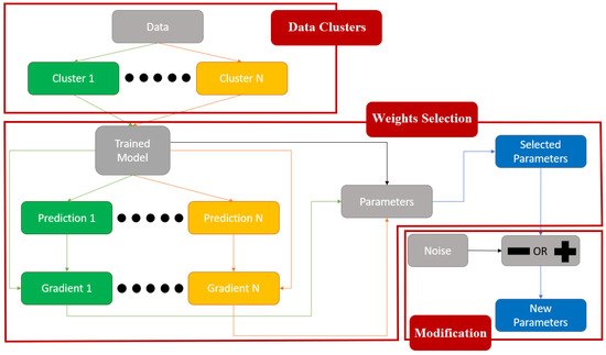
Figure 2.
The process followed by the attack we developed and implemented in this work.
Note that if only a few parameters are manipulated, the attack is less likely to be detected and will be more efficient. Moreover, there are other variables to qualify the threat developed, such as quantification of the modification (noise) added to the weight and the model’s decrease in accuracy.
In the rest of this section, the steps to generate the general fault injection attack are detailed.
3.1. Identifying Input Data Clusters
With the intuition that the model should act equally for similar data, first, a cluster analysis is performed on input data. The attacker focuses on the similarity analysis between the selected subset of the input data where he/she is attacking. In this paper, the model’s behavior refers to activations when specific input is injected into the model, taking into account the connections between neurons. From this point of view, depending on the input sample, the model behaves differently because the neuron activations are different in each case. For this reason, when two input samples are similar, it is expected that the model should behave similarly, activating the same subset of neurons. The activation value of a neuron depends on its inputs and its weights. By studying the similarities between activation values of different input data and cluster divisions found in the analyzed data, it is possible to detect the most influential neurons in the classification of the selected subset. With this information, the attacker should be able to choose specific weights of the model towards which to direct the attack. Thus, by manipulating those particular parameters, the attacker can misclassify the selected cluster of images while leaving the others classified correctly.
In supervised machine learning, the input data is labeled with different classes, and the target model learns to classify them by detecting the patterns associated with each input sample. The model’s objective is to learn to group the data into classes, i.e., it modifies its weights to classify the detected patterns correctly. That may mean that some weights are specialized to classify particular patterns, concretely tying some specific items to a class. The first possible clusters the attacker would consider are the model classes themselves. If there is some way to detect the most influential weights based on the class selected to be misclassified, the attacker could modify those to carry out the attack.
However, misclassification can be more specialized, since within the same class, the model can contain different behaviors, and the influential neurons of those behaviors mix. Therefore, a study of clusters (similar instances) in the data can considerably specialize the attack, as the effectiveness of the attack depends on misclassifying the desired set without altering the prediction of the others. Therefore, by reducing the amount of influential weights, the attack area is smaller and more distinct, making the attack less detectable. These clusters of input data can be obtained by various similarity measures, such as Euclidean distance [24], Hamming distance [25], mean square error [26], maximum signal-to-noise ratio [27], and structural similarity [28].
3.2. Selection of the Most-Influential Weights
The main challenge of selecting the weights to be modified is that they can also affect the prediction of other input sets (different from the selected ones), making the model attack evident. Therefore, optimizing the chosen modifications in the parameters is necessary to carry out this attack efficiently.
There are several ways to perform this selection, such as centering the search to a specific layer [18] or by analyzing the sensibility of the weights in the model [21]. In this work, following the evasion attack approach, parameters are chosen by how the gradient of the input data influences predictions. This gradient indicates how important a feature of the input data is, i.e., it can be considered a metric to select the position of the most-relevant data of the input layer (input neuron). In this regard, it should be noted that each input neuron is usually assigned more than one weight by the next layer. Therefore, once the input neurons have been chosen, the attacker must set the upper limit quantity indicating the maximum number of weights to be selected for pursuing the attack. Moreover, a metric is necessary to select this quantity from the assigned parameters. In this work, this subset of parameters is generated according to the absolute values of the weights, taking the highest ones.
In summary, this approach starts by detecting the most-relevant input neurons of the input layer through the gradient. Among the weights assigned to those features, the ones with the highest absolute values are defined as the most influential ones. This subset is used for generating the attack.
3.3. Modification of the Selected Weights
Once the critical parameters are selected, noise is added to obtain the desired misclassification. That modification is incorporated step-by-step to observe the effect of such manipulation on the chosen weights. Moreover, adding less noise in several steps makes the attack more optimized since the manipulated weights will be more similar to the original ones, i.e., the attack will be less perceptible. The magnitude of the noise added in each step is defined by the parameter , and the number of steps is indicated by the parameter s. Therefore, the upper limit of the difference between the original weight value and the modified one is .
As mentioned above, the gradient indicates the impact each input feature has on the prediction of the target neural network. In the training phase of a neural network, its weight gradients are calculated. Those values are subtracted from the previous value of the parameters, causing model learning. In other words, the subtraction of the gradient generates model learning while the addition would imply a step backwards in the learning (i.e., the model would unlearn). Therefore, when a value of the same sign of the gradient is subtracted from the weight, it makes that weight gain more important in the prediction, while addition would make that parameter lose strength.
With this in mind, assuming that the attacker wants to misclassify one of the clusters, they can follow two different strategies. On the one hand, one can weaken the impact of the most-influential weights of the target cluster by adding the multiplication of the selected noise by the sign of the corresponding gradients. With previous modifications, the attacker would make those weights have a lower impact on the prediction, achieving misclassification of the cluster. On the other hand, the second strategy strengthens the most-influential parameters associated with the rest of the clusters. This is accomplished by subtracting the multiplication of the noise by the sign of the corresponding gradients. In this way, these weights would gain impact in the prediction, transferring data from the target cluster to the other clusters.
The second approach could lead to worse results because it can modify some weights without control. For example, assuming a dataset A containing three different clusters, , where is the selected weights assigned to , and is the targeted cluster to misclassify. Then, the second method would modify and , strengthening those weights and converting elements from to or . However, items from could convert to and vice versa since strengthening of and affects to and , respectively. That would not happen with the first method because it is more focused on , reducing the impact of , which directly affects .
4. Experiment
In this work, the proposed new version of the weight modification attack was implemented to the targeted model, a classifier of cancerous and non-cancerous breast tissues. The model is composed of a convolutional part and a dense part; the convolutional block is in charge of extracting features from the input data, whereas the dense part classifies those data using the computed features. In this experiment, the goal is to misclassify a targeted cluster by modifying the weights of the first layer of the dense block.
First, this section describes the dataset used for the analysis. Next, the model selected to be attacked is detailed. Then, the experiment is described, detailing how the attack is managed. Finally, configuration parameters of the experiment are shown.
4.1. Dataset
The Breast Histopathology Images dataset has been used for this experiment. Breast cancer is the most common form of cancer in women, and invasive ductal carcinoma (IDC) is the most common form of breast cancer. The dataset consists of 277,524 patches of size 50 × 50 of breast tissues with 198,738 IDC negative and 78,786 IDC positive [29,30]. Moreover, those images are labeled by zero (IDC negative) if the tissue does not have cancer and one (IDC positive) if cancer is present. This dataset (https://www.kaggle.com/paultimothymooney/breast-histopathology-images, accessed on 5 April 2022) is open-access, and it contains 2 GB of images.
For the experiment, the dataset is divided into two subsets: training data (70%) and test (30%) data, as is usual in this type of study [31,32]. A stratified train–test split is used to preserve proportions of classes from the original dataset. The training dataset is used to train the model detailed in Section 4.2, while the test data is used to measure the obtained results of the experiment.
4.2. Model
The analyzed model is a convolutional neural network. It is built by the convolutional block of the VGG16 neural network and a multi-layer perceptron (MLP) model. In total, the complete model contains 21 layers (Table 1), and the first 18 layers (VGG16 part) are pre-trained using the ImageNet dataset. The completed model was trained with the dataset presented in Section 4.1, thus it learned to classify the breast tissue images.

Table 1.
Target model structure.
4.3. Weight Modification
In this work, the attack exploits the dense part of the detailed model; specifically, the first fully connected layer is the target of the weight modification attack. Briefly, we start by searching different image clusters from the breast cancer image dataset presented in Section 4.1. For each clustering, the attack described in Section 3 is applied and the results are discussed in Section 5.
Once the model is trained, 2000 well-classified images (1000 per class) are selected randomly from the test data. The misclassified images are discarded from the test data since the internal behavior of the model is different or abnormal in those cases. This selected subset of images is separated by classes, generating two initial clusters. Next, the feature vectors of the images are obtained through the convolutional network (Figure 3). In this case, the first layer of the dense part is considered the targeted layer. The output of the convolutional block is a feature vector, where the output values of the convolutional layers from the vector are assigned to an input neuron of the dense block. Therefore, if the most-influential features in the prediction are known, the input neurons with the highest impact are detected. With this in mind, the influence of the densest input neurons is studied through the computed feature vectors.
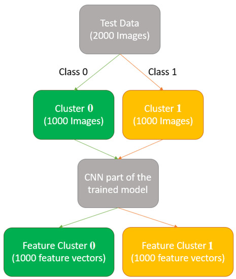
Figure 3.
The process of cluster and feature obtention.
The gradient is used as a metric of prediction impact to obtain the most-influential, densest input neurons. Once all gradients are calculated, two sets of the same size of gradient vectors are obtained (Figure 4). Note that a gradient vector of the same dimension is obtained for each feature vector. Each group contains various important values of the input neurons. Specifically, one value is assigned to a neuron for each gradient vector in the gradient set. Since a single value per feature is desired, the mean of the absolute value of all gradients associated with an input neuron is selected as a representative value indicating the impact level of the feature. Therefore, a single gradient vector is computed from each gradient set. The values of these vectors indicate the importance of the input features in predicting the selected cluster. Both clusters can share some highly influential features, but modifying the corresponding weights could also misclassify unwanted input data. Therefore, when choosing meaningful attributes for generating the attack on the specified cluster, it is essential to discard the features shared with the rest of the clusters (Figure 5).
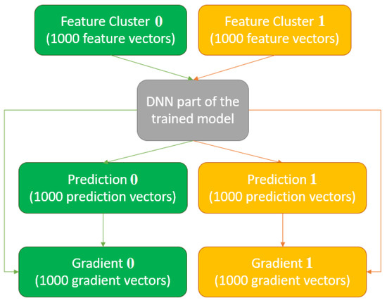
Figure 4.
The process to obtain the gradient per cluster.
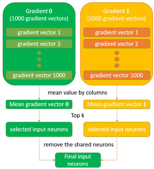
Figure 5.
The process to select the input neurons with highest impact on the prediction.
In the model used for the experiment, the input layer interacts with 131,072 (512 × 256) weights, where 256 are associated with each input neuron. So once the most-influential neurons are selected, note that 256 specific weights could be modified for each one. Therefore, the highest values in each row were selected, obtaining the final weights to be manipulated. In other words, influential weights are chosen for each defined cluster. However, the shared influential weights (the parameters that appear as influential in more than one cluster) are removed, maintaining influential weights associated with the cluster i.
With the influential weights selected for each defined cluster, an attempt is made to misclassify each image from the selected cluster. Both strategies described in Section 3 are used, i.e., adding noise to the parameters associated with the cluster to be misclassified and subtracting noise from the weights associated with the clusters that we do not want to manipulate. Each of these methods obtains different results for each class, which are presented and discussed in Section 5.
4.4. Experiment Parameters
The experiment depends on the configuration of the following parameters that allow varying numbers of modified weights, the targeted cluster, and the strategy used:
- k:= the upper limit of the number of modified weights.
- := the cluster n to be misclassified, where .
- := the method used to incorporate the noise, where . Note that, indicates the summation method and indicate the subtraction method.
- := magnitude of the noise added in each step.
- s:= number of steps used to generate the attack.
Moreover, these parameters define a configuration , where the attack is implemented with k modified weights, indicates the method used, with the target cluster using magnitude noise and s number of steps. For each configuration, the accuracy of each cluster defined in the input data is shown in Section 5. Suppose that is the attacked model and are the original labels of the elements in a certain cluster , then
is the result of the for the configuration . Defining C as the cluster with the complete input data, suppose is the set of defined clusters of the input data, and the configuration is used to generate the attack, then
is the main result of the analysis of the configuration. Observe that it is in the interval . Note that, when the result decreases, increases, and vice-versa if the result increases. Moreover, if the decreases, decreases, and vice-versa. Therefore, a high value means that the attack is misclassifying mostly the target cluster, and a low value means that the attack is misclassifying mostly the rest of the defined clusters. In other words, the objective of the attacker is to achieve as high a value of as possible.
5. Results and Discussion
In this work, with the goal of avoiding an excessive number of options, the parameters and s are fixed at and 500, respectively. Therefore,
As mentioned in Section 4, in this case, the classes are taken as clusters. That is why the investigation is divided into two main analyses, and , where refers to the cluster of class 0 and refers to the cluster of class 1.
The experiment begins by analyzing . Table 2 shows the results from varying k and . Concerning k, all integers between (26, 14,400) are tested, but the results shown in the table are selected according to the highest values of and . The five highest results of each are shown.
Table 2.
The best results obtained in the analysis .
Therefore, Table 2 shows that in both strategies, and , the accuracy of is successfully reduced. However, the summation method achieves better results by misclassifying and keeping the accuracy of unmutated. Moreover, was monitored (Figure 6) during the noise incorporation process. Figure 6 shows how evolved when noise was added to the weights. It can be noticed how the initial modification has a high impact, while as more noise is added, there is less impact on the accuracy. It even reaches the point where new noise no longer impacts the predictions.
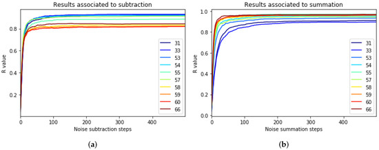
Figure 6.
Monitoring of (a) and (b) during the noise addition process.
In the case of analyzing , Table 3 shows the best results obtained from and for different values of k. The top five were selected from each one according to .
Table 3.
This table shows the best results obtained in the analysis .
Table 3 shows that the attack manages to successfully reduce the accuracy of in both strategies, and . However, in this case, the subtraction method achieves better results by misclassifying while keeping the accuracy of unchanged. Moreover, was monitored (Figure 7) during the noise incorporation process. Figure 7 shows how evolved when the noise was being added to the weights. It can be noticed how the initial modification has a high impact, while as more noise is added, it has less impact on accuracy. It even reaches the point where new noise no longer impacts the predictions.
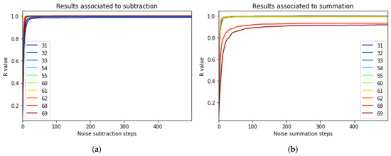
Figure 7.
The monitoring of (a) and (b) during the noise addition process.
Comparing both and , the results are similar. However, in , performs the best, while in , has the best results. Moreover, there exists a small gap between the results of and . Thus, the attack is more successful when misclassifying . This may be because the model classifies class 0 images better than class 1 images. Such knowledge could help the attacker decide what cluster to attack.
Deeper Clusterization
Once the previous attacks are analyzed, other clusters are searched in the already defined clusters and in order to develop a more guided and precise attack. Supposing , the goal is to find and misclassify a new subcluster while the others, and , are well-classified. Notice that,
and
The first method to detect is by visualization implemented through the PCA algorithm [33], which may help us find possible subclusters inside and . The proposed visualization is applied to the complete set of data to check if clusters and are distinguishable (Figure 8). The color of the visualization represents the mean distance of specific input data to the other samples. For visualization generation, the Hamming and the Euclidean distances are tested in the plots.
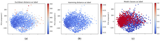
Figure 8.
The projection of the feature vectors generated by the PCA algorithm: (a) colors the dots using Euclidean distance, while (b) colors the dots by Hamming distance. In addition, (c) shows how the elements of each class are distributed, where the blue ones are labeled by zero and the red ones are labeled by one.
Figure 8a with the Euclidean distance shows possible separation between two cluster that may coincide with the Figure 8c, where the color is labeled by model classes. Meanwhile, if the Hamming distance is used (Figure 8b), no differentiated subsets are found. For this reason, the visualization based on Euclidean distance is implemented to try to find subclusters in each (Figure 9).
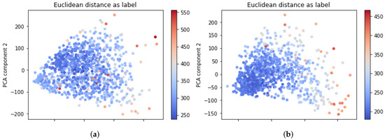
Figure 9.
The projection of the feature vectors generated by the PCA algorithm: (a) represents the elements from and (b) represents the elements from .
Plots in Figure 9 show possible subclusters in and , respectively. If darker samples are grouped in a concrete zone, this could be interpreted as desired subclusters. Thus, two algorithms based on Euclidean distance are implemented to isolate those possible subsets: K-means [34] and DBSCAN [35]. However, neither K-means nor DBSCAN can separate those possible subclusters successfully. Every generated did not have any particular influential weight compared to . In other words, the values obtained in and with n in were less than , i.e., the attacks were not successfully pursued, requiring further research and a more complex approach.
6. Conclusions and Future Work
This work presents a new version of the weight modification attack. Moreover, it was proven that it successfully attacks the clusters formed by the model’s classes. Both classes of images are misclassified, reducing their accuracy considerably. Notably, cluster one, which began with 100% accuracy, ended with 0% accuracy, while cluster zero maintained 100% accuracy. In the same way, attacking cluster zero, initial accuracy was successfully reduced to 2.7% while maintaining the other cluster’s accuracy at 100%. Therefore, this investigation presents a successful new version of the fault injection attack, showing a possible threat that a deep learning model can contain.
This paper presents the proof-of-concept in a model with two classes with a specific dataset. However, the presented attack could be implemented for a model with more classes or with other datasets. In the same way, it may be good to misclassify smaller subclusters to increase the focus of the attack, but this must be demonstrated in future work. These cluster-detection methods can continue to be investigated and analyzed to determine if the identified clusters can specialize the attack. Moreover, other strategies to define clusters can be presented and studied. For example, another method to detect those clusters could be via the model’s behavior, focusing on activation of the neurons.
The experiments in this paper only analyzed the sensitivity of the parameter k. Future work to be considered includes analyzing the effects of modifying the rest of the attack configuration parameters. Furthermore, in the presented version, the attacker manually selects the layer used for the attack without further information about the vulnerability of the parameters in that layer. An initial cross-layer analysis could be formulated to optimize the success of the attack and guide the attacker to optimize layer selection.
Author Contributions
X.E.-B. and A.G.-L. designed and implemented the experimental testbed and algorithm. R.O.-U. and I.M. supervised the experimental design and managed the project. R.O.-U. and I.M. reviewed the new approach of this research. X.E.-B. performed the experimental phase. All authors contributed to the writing and reviewing of the present manuscript. All authors read and agreed to the published version of the manuscript.
Funding
This research has been partially funded by European Union’s Horizon 2020 research and innovation programme project SPARTA and by the Basque Government under ELKARTEK project (LANTEGI4.0 KK-2020/00072).
Institutional Review Board Statement
Not applicable.
Informed Consent Statement
Not applicable.
Data Availability Statement
Not applicable.
Conflicts of Interest
The authors declare no conflict of interest.
References
- Finlayson, S.G.; Bowers, J.D.; Ito, J.; Zittrain, J.L.; Beam, A.L.; Kohane, I.S. Adversarial attacks on medical machine learning. Science 2019, 363, 1287–1289. [Google Scholar] [CrossRef] [PubMed]
- Sharma, P.; Austin, D.; Liu, H. Attacks on machine learning: Adversarial examples in connected and autonomous vehicles. In Proceedings of the 2019 IEEE International Symposium on Technologies for Homeland Security (HST), Woburn, MA, USA, 5–6 November 2019; pp. 1–7. [Google Scholar]
- Akhtar, N.; Mian, A. Threat of adversarial attacks on deep learning in computer vision: A survey. IEEE Access 2018, 6, 14410–14430. [Google Scholar] [CrossRef]
- Deng, Y.; Zhang, T.; Lou, G.; Zheng, X.; Jin, J.; Han, Q.L. Deep learning-based autonomous driving systems: A survey of attacks and defenses. IEEE Trans. Ind. Inform. 2021, 17, 7897–7912. [Google Scholar] [CrossRef]
- Chakraborty, A.; Alam, M.; Dey, V.; Chattopadhyay, A.; Mukhopadhyay, D. A survey on adversarial attacks and defences. CAAI Trans. Intell. Technol. 2021, 6, 25–45. [Google Scholar] [CrossRef]
- Mozaffari-Kermani, M.; Sur-Kolay, S.; Raghunathan, A.; Jha, N.K. Systematic poisoning attacks on and defenses for machine learning in healthcare. IEEE J. Biomed. Health Inform. 2014, 19, 1893–1905. [Google Scholar] [CrossRef] [PubMed]
- Yang, C.; Wu, Q.; Li, H.; Chen, Y. Generative poisoning attack method against neural networks. arXiv 2017, arXiv:1703.01340. [Google Scholar]
- Biggio, B.; Pillai, I.; Rota Bulò, S.; Ariu, D.; Pelillo, M.; Roli, F. Is data clustering in adversarial settings secure? In Proceedings of the 2013 ACM Workshop on Artificial Intelligence and Security, Berlin, Germany, 4 November 2013; pp. 87–98. [Google Scholar]
- Corona, I.; Giacinto, G.; Roli, F. Adversarial attacks against intrusion detection systems: Taxonomy, solutions and open issues. Inf. Sci. 2013, 239, 201–225. [Google Scholar] [CrossRef]
- Jiang, W.; Li, H.; Liu, S.; Luo, X.; Lu, R. Poisoning and evasion attacks against deep learning algorithms in autonomous vehicles. IEEE Trans. Veh. Technol. 2020, 69, 4439–4449. [Google Scholar] [CrossRef]
- Lee, S.J.; Yoo, P.D.; Asyhari, A.T.; Jhi, Y.; Chermak, L.; Yeun, C.Y.; Taha, K. IMPACT: Impersonation attack detection via edge computing using deep autoencoder and feature abstraction. IEEE Access 2020, 8, 65520–65529. [Google Scholar] [CrossRef]
- Globerson, A.; Roweis, S. Nightmare at test time: Robust learning by feature deletion. In Proceedings of the 23rd International Conference on Machine Learning, Pittsburgh, PA, USA, 25–29 June 2006; pp. 353–360. [Google Scholar]
- Fredrikson, M.; Jha, S.; Ristenpart, T. Model inversion attacks that exploit confidence information and basic countermeasures. In Proceedings of the 22nd ACM SIGSAC Conference on Computer and Communications Security, Denver, CO, USA, 12–16 October 2015; pp. 1322–1333. [Google Scholar]
- Shokri, R.; Stronati, M.; Song, C.; Shmatikov, V. Membership inference attacks against machine learning models. In Proceedings of the 2017 IEEE Symposium on Security and Privacy (SP), San Jose, CA, USA, 22–24 May 2017; pp. 3–18. [Google Scholar]
- Ateniese, G.; Mancini, L.V.; Spognardi, A.; Villani, A.; Vitali, D.; Felici, G. Hacking smart machines with smarter ones: How to extract meaningful data from machine learning classifiers. Int. J. Secur. Netw. 2015, 10, 137–150. [Google Scholar] [CrossRef]
- Nguyen, T.N. Attacking Machine Learning models as part of a cyber kill chain. arXiv 2017, arXiv:1705.00564. [Google Scholar]
- Wang, B.; Gong, N.Z. Stealing hyperparameters in machine learning. In Proceedings of the 2018 IEEE Symposium on Security and Privacy (SP), Francisco, CA, USA, 21–23 May 2018; pp. 36–52. [Google Scholar]
- Liu, Y.; Wei, L.; Luo, B.; Xu, Q. Fault injection attack on deep neural network. In Proceedings of the 2017 IEEE/ACM International Conference on Computer-Aided Design (ICCAD), Irvine, CA, USA, 13–16 November 2017; pp. 131–138. [Google Scholar] [CrossRef]
- Zhao, P.; Wang, S.; Gongye, C.; Wang, Y.; Fei, Y.; Lin, X. Fault sneaking attack: A stealthy framework for misleading deep neural networks. In Proceedings of the 2019 56th ACM/IEEE Design Automation Conference (DAC), Las Vegas, NV, USA, 2–6 June 2019; pp. 1–6. [Google Scholar]
- Rakin, A.S.; He, Z.; Li, J.; Yao, F.; Chakrabarti, C.; Fan, D. T-bfa: Targeted bit-flip adversarial weight attack. IEEE Trans. Pattern Anal. Mach. Intell. 2021. [Google Scholar] [CrossRef] [PubMed]
- Tsai, Y.L.; Hsu, C.Y.; Yu, C.M.; Chen, P.Y. Formalizing Generalization and Adversarial Robustness of Neural Networks to Weight Perturbations. In Proceedings of the NeurIPS Thirty-Fifth Annual Conference on Neural Information Processing Systems, Virtual, 6–14 December 2021; Volume 34. [Google Scholar]
- Weng, T.W.; Zhao, P.; Liu, S.; Chen, P.Y.; Lin, X.; Daniel, L. Towards certificated model robustness against weight perturbations. In Proceedings of the AAAI Conference on Artificial Intelligence, New York, NY, USA, 7–12 February 2020; Volume 34, pp. 6356–6363. [Google Scholar]
- Wang, X.; Wang, S.; Chen, P.Y.; Wang, Y.; Kulis, B.; Lin, X.; Chin, S. Protecting Neural Networks with Hierarchical Random Switching: Towards Better Robustness-Accuracy Trade-off for Stochastic Defenses. In Proceedings of the Twenty-Eighth International Joint Conference on Artificial Intelligence (IJCAI-19), Macao, China, 10–16 August 2019; pp. 6013–6019. [Google Scholar] [CrossRef] [Green Version]
- Singh, A.; Yadav, A.; Rana, A. K-means with Three different Distance Metrics. Int. J. Comput. Appl. 2013, 67, 13–17. [Google Scholar] [CrossRef]
- Norouzi, M.; Fleet, D.J.; Salakhutdinov, R.R. Hamming distance metric learning. In Proceedings of the NeurIPS Twenty-Sixth Annual Conference on Neural Information Processing Systems, Lake Tahoe, NV, USA, 3–6 December 2012; Volume 25. [Google Scholar]
- Judd, D.; McKinley, P.K.; Jain, A.K. Large-scale parallel data clustering. IEEE Trans. Pattern Anal. Mach. Intell. 1998, 20, 871–876. [Google Scholar] [CrossRef] [Green Version]
- Abramovich, Y.I. A controlled method for adaptive optimization of filters using the criterion of maximum signal-to-noise ratio. Radio Eng. Electron. Phys. 1981, 26, 87–95. [Google Scholar]
- Gentner, D.; Markman, A.B. Defining structural similarity. J. Cogn. Sci. 2006, 6, 1–20. [Google Scholar]
- Cruz-Roa, A.; Basavanhally, A.; González, F.; Gilmore, H.; Feldman, M.; Ganesan, S.; Shih, N.; Tomaszewski, J.; Madabhushi, A. Automatic detection of invasive ductal carcinoma in whole slide images with convolutional neural networks. In Medical Imaging 2014: Digital Pathology; SPIE: Bellingham, WA, USA, 2014; Volume 9041, p. 904103. [Google Scholar]
- Janowczyk, A.; Madabhushi, A. Deep learning for digital pathology image analysis: A comprehensive tutorial with selected use cases. J. Pathol. Inform. 2016, 7, 29. [Google Scholar] [CrossRef] [PubMed]
- Reitermanova, Z. Data splitting. In Proceedings of the WDS 2010, Prague, Czech Republic, 1–4 June 2010; Volume 10, pp. 31–36. [Google Scholar]
- Krittanawong, C.; Johnson, K.W.; Rosenson, R.S.; Wang, Z.; Aydar, M.; Baber, U.; Min, J.K.; Tang, W.W.; Halperin, J.L.; Narayan, S.M. Deep learning for cardiovascular medicine: A practical primer. Eur. Heart J. 2019, 40, 2058–2073. [Google Scholar] [CrossRef] [PubMed]
- Ding, C.; He, X. Principal component analysis and effective k-means clustering. In Proceedings of the 2004 SIAM International Conference on Data Mining, Lake Buena Vista, FL, USA, 22–24 April 2004; pp. 497–501. [Google Scholar]
- Pham, D.T.; Dimov, S.S.; Nguyen, C.D. Selection of K in K-means clustering. Proc. Inst. Mech. Eng. Part C J. Mech. Eng. Sci. 2005, 219, 103–119. [Google Scholar] [CrossRef] [Green Version]
- Deng, D. DBSCAN clustering algorithm based on density. In Proceedings of the 2020 7th International Forum on Electrical Engineering and Automation (IFEEA), Hefei, China, 25–27 September 2020; pp. 949–953. [Google Scholar]
Publisher’s Note: MDPI stays neutral with regard to jurisdictional claims in published maps and institutional affiliations. |
© 2022 by the authors. Licensee MDPI, Basel, Switzerland. This article is an open access article distributed under the terms and conditions of the Creative Commons Attribution (CC BY) license (https://creativecommons.org/licenses/by/4.0/).