Unsupervised Driving Situation Detection in Latent Space for Autonomous Cars

Abstract

A policy determines the action that an autonomous car needs to take according to its current situation. For example, the car keeps itself on track or overtakes another car, among other policies. Some autonomous cars could need more than one policy to drive appropriately. In those systems, the behavior selector subsystem selects the policy that the car needs to follow. However, in the current literature, there is not a unified way to create these policies. In most cases, the amount and definition of the policies are hand-engineering using the information taken from observations and the knowledge of the engineers. That paradigm requires a lot of human effort. Additionally, there is human subjectivity due to the hand labeling. Furthermore, the experts could not agree about the number of existing situations and the boundaries between policies (the point at which one situation turns into another). To deal with the subjectivity of setting the number and definition of policies, we propose a novel approach that uses the “divide and conquer” paradigm. This method first, sets the number of required policies by clustering previous observations into situations, and second, it configures a regression-based policy for each situation. As a result, (i) the method can detect driving situations from raw data automatically using unsupervised algorithms, helping to avoid the hand-engineering made by an expert, and (ii) the method creates relatively small and efficient policies without human intervention using behavioral cloning. To validate the method, we have collected a custom dataset in simulation and we have conducted several experiments comparing the performance of our proposal versus two state-of-the-art end-to-end methods. Our results show that our method outperforms the end-to-end approaches in terms of a bigger R square metric (0.19 over the tested methods) and a lower mean squared error (0.48 below the tested methods).

1. Introduction

The development of autonomous cars is a topic of interest for many groups, among them being the scientific community and the automotive and technology industries [1]. Autonomous cars are characterized by their complexity and work in completely dynamic and changing environments; this is why the general system is subdivided into different subsystems in charge of solving particular tasks. Inside the general architecture of an autonomous car, there is a subsystem named the behavior selector [2], also known as the policy selector, which chooses the behavior that a car needs to follow from a set of predefined policies. Among the multiple tasks, this subsystem considers the current driving behavior and tries to avoid collisions with static and moving obstacles in the environment. The polices determine the actions that an autonomous car needs to take according to an observation of the car. Some examples of these polices are lane keeping, overtaking another car, changing lanes, intersection handling, and traffic light handling, among others. An autonomous car must deal with any context, and for this reason the detection of different driving situations is necessary. So, we can say that the policies are assigned according to the situation that the car is facing. In general, those driving situations cluster observations of the car that are similar. Some examples of these driving situations are when the car is facing a curve, when there are cars nearby, and when it is centered in the lane, among others.

According to our literature review, there is no unified way to create the policies that are used in the behavior selectors. In most cases, the policies are engineered by hand in two steps: First, the designers manually define a set of driving situations according to their expertise. Then, they define the policies that best suit each driving situation. The previous processes require a lot of effort. Additionally, there is a lot of subjectivity due to the manual labeling and because experts do not always agree on the number of situations and the decision boundaries between situations (the point at which one situation turns into another).

For example, in the case of Buehler et al. [3] and Jo et al. [4] all the states or driving situations are hand-engineered, and in total, 13 possible situations are considered for selecting different policies, such as forward driving, lane keeping, obstacle avoidance, U-turning, intersection handling, and stopping, among others. One problem is the difficulty of modeling complex scenarios because non-controlled environments are considerably more complicated than what the cars face in the competitions such as the Urban Challenge; in consequence, a method to select an appropriate number of situations is necessary, and it is also necessary to define each driving policy. In the work of Galceran et al. [5], a behavior-selection approach is proposed that models the car behavior as well as the nearby cars’ potential intentions as a discrete set of policies. They used a set of hand-engineering policies to in-lane and intersection driving situations. The idea of assuming finite sets of policies to speed up planning has appeared previously [6,7,8]. Similarly, they propose designing a set of policies that are readily available at planning time. The idea of dividing behaviors into policies appears to be a good solution to accelerate the planning and execution of the behavior selector. Now, thanks to the advantages of Deep Learning techniques [9,10], in recent years, a large variety of Behavioral Cloning Techniques imitate how a human pilot can drive [11,12,13,14]; however, it is necessary to label the data. In some cases, such as in end-to-end systems, the actions are the labels, and in some other intermediate systems, the driving situations are the needed labels [15] or can have intermediate detections of objects in the scenes [16,17]. However, the task of labeling the data is hand-engineered, and the subjectivity probably affects the performance of the system.

In this paper, we propose a method for estimating the amount of policies and their automatic creation. For this purpose, we developed an unsupervised method that clusters the latent space representation of the observations into driving situations. Then, we assign a driving policy to each situation. A latent space, also known as latent feature space or embedding space, is a representation of compressed data. The latent space helps to learn the features of data and simplifies data representations for the purpose of finding patterns. We use a neural network autoencoder to obtain the latent space representation. The encoding part is in charge of extracting all the main features from the input image. With respect to the policies, we propose to generate them as a behavioral cloning but using only the data that correspond to its cluster.

As a result, our method can detect driving situations from raw data automatically, helping to avoid the hand-engineering process performed by an expert. From these driving situations, the method also creates policies without human intervention using behavioral cloning. In our experiments, we found that this method overcomes a global driving policy in terms of determination score for several simulation scenarios. Finally, our proposed method can be implemented in a behavior selector for autonomous cars, as shown in Figure 1.

The rest of the paper is presented as follows. Section 2 describes the “divide and conquer” methodology, as well as a review of recent approaches. Section 3 details the preliminaries, where we address the problem and a general overview of the solution. In Section 4, we describe in detail the methodology of the presented work. Section 5 tests the methodology and compares the obtained results between a global driving policy and individual driving policies partitions. Finally, Section 6 presents our conclusions.

2. Related Work

In approaches such as the one presented by Okumura et al. [18] from the Toyota Research Institute, they only consider roundabout situations; in the work of Mihaly et al. [19], they only consider intersections scenarios. In these works, only one type of driving situation is considered, roundabouts or intersections. It works properly only for a reduced scenario, but it is necessary to have more policies to scale to all the different driving situations that a car faces while it is in use. In other methodologies, as presented by Aeberhard et al. [20], the authors try to reduce the complexity of the model dividing the driving task into a finite set of lateral and longitudinal driving situations (guidance states). They first, evaluate the driving situation and then produce a driving request which outputs a series of discrete events to evaluate by the Deterministic Automaton. Although there have been major improvements, all aspects of the automated driving system, including perception, localization, decision-making, and path planning algorithms, still need to be further developed to bridge the gap between robotics research and a customer-ready system. It is necessary to increase the number of driving situations to model under different scenarios. Other approaches, such as in the works of Thrun et al. [21] and Ulbrich et al. [22], apply POMDP to behavior selection in order to perform lane changes while driving in urban environments. They used a finite set of policies to speed up planning. In Brechtel et al. [8], their approach is used to deal with potentially hidden objects and observation uncertainties. All have in common that using a finite set of policies can speed up planning, which is a good idea to solve the general driving problem and demonstrate the importance of the number selection of policies. There are different approaches where the data are divided into specialized subsets in which there is a similitude trying to solve different problems applying the “divide and conquer” technique. This method is shown to be useful to accelerate the process of learning for some algorithms. For example, in the study of Zhou et al. [23], they propose an efficient “divide and conquer” model, which constrains the loss function of Maximum Mean Discrepancy (MMD) to a tight bound on the deviation between an empirical estimate and expected value of MMD and accelerates the training process. This approach contains a division step and a conquer step. In the division step, they learn the embedding of training images based on an autoencoder and partition the training images into adaptive subsets through K-means clustering based on the embedding. In the conquer step, sub-models are fed with subsets separately and trained synchronously. Experimental results show that with a fixed number of iterations, this approach can converge faster and achieve better performance compared with the standard MMD-GANs. In other computational research areas, such as in Reinforcement Learning, designing a good reward function is essential to problems such as robot planning, and it can be challenging. The reward needs to work across multiple different environments, and that often requires many iterations of tuning. In the approach of Ratner et al. [24], they introduce a “divide and conquer” model that enables the designer to specify a reward separately for each environment. They conduct user studies in an abstract grid world domain and in a motion-planning domain for a 7-DOF manipulator that measures user effort and solution quality. The solution demonstrates that this method is faster, easier to use, and produces a higher-quality solution than the typical method of designing a reward jointly across all environments. Wang et al. [25] propose a deep neural network model based on a semantic “divide and conquer” approach, they decompose a scene into semantic segments, such as object instances and background stuff classes, and they predict a scale and shift-invariant depth map for each semantic segment in canonical space. Semantic segments of the same category share the same depth decoder, so the global depth prediction task is decomposed into a series of category-specific ones, which are simpler to learn and easier to generalize to new scene types. Even Kim et al. [26] proposed a “divide and conquer” contour design methodology using a bioinspired design methodology for a multifunctional lever based on the morphological principle of the lever mechanism in the Salvia pratensis flower.

These kinds of solutions motivate us as a research group to ask us the following questions: How can we avoid subjectivity in the labeling of the data? How can we select an adequate number of policies from the dataset? Finally, how can we avoid the manual labeling of the data?

In the above-mentioned cases, the “divide and conquer” technique shows that there is a similitude with the idea of dividing the data into driving situations and trying to cluster similar data to accelerate the process of the learning of different policies according to driving situations. The idea of dividing the data into specialized subsets in an unsupervised manner could be a solution to avoid the subjectivity of a person labeling the data and avoids spending a lot of time making the hand-engineered labeling. It also speeds up the process of learning with the specialized subsets to train the individual policies.

3. Preliminaries

In this section, we provide the addressed problem and a general overview of the solution. First, we assume that the vehicle is a car-like robot whose state, $x\in X$, is defined as its position and velocity with respect to the body frame. In a formal way, the state is defined as follows:

$$x=[x,y,v_x,v_y]$$

(1)

where x and y define the body frame, $v_x$ is the speed of the car along the longitudinal axis of the car, and $v_y$ is the speed of the car along the transverse axis of the car.

An observation of the car, $z\in Z$, is the set of reading from the sensors. In particular, our car is capable of obtaining the following readings:

$$z=[Im,\theta ,\beta ,rpm,track]$$

(2)

where each element is described in

Table 1. Observation space of the car. These are the elements that can be read from the car’s sensors.

Elements	Observations	Range
$Im$	Image	${\mathrm{I}\mathrm{R}}^{224\times 224\times 3}$
$\theta$	The angle between car direction and the direction of track axis	$[-\pi ,\pi ]$
$\beta$	Gear	{−1, 0, …, 6}
$rpm$	Number of rotations per minute of the car engine	$\mathrm{I}\mathrm{R}$
$track$	Distance between the car and the track axis	$\mathrm{I}\mathrm{R}$

.

The car can change its state by applying an action, $a\in A$. In this work, the action is a vector of four elements:

$$a=[accel,break,clutch,gear,steering]$$

(3)

where each element is defined in

Table 2. Action space of the car. These are the elements that can be controlled in the car.

Elements	Actions of the Car	Range
$accel$	Accelerator pedal	[0, 1]
$break$	Break pedal	[0, 1]
$clutch$	Clutch pedal	[0, 1]
$gear$	Gear	{−1, 0, …, 6}
$steering$	Steering wheel angle	$[-\pi ,\pi ]$

.

Previous works solved the problem of autonomous driving [27,28] by defining a global policy, $\Pi$, which is a function that takes the image coming from the observations of the car and maps it directly to the action set, formally:

$$\Pi (z,x):Z\times X\to A$$

(4)

However, one problem of the global driving policy occurs when it is trained with a small amount of data of a single driving situation, because the driving policy cannot learn the appropriate responses and it might ignore what it has to do because of the reduced probability of this driving situation to happen.

Our hypothesis is that several specialized policies can be learned easier and can achieve better results.This is because the data are similar under the same context. So, instead of a global policy, in Equation (4), we propose to split it into several ones, i.e.:

$$\Pi \approx \{{\pi }_1,{\pi }_2,{\pi }_3,\dots {\pi }_n\}$$

(5)

where ${\pi }_n$ is the nth driving policy. So that, $\Pi$ can be approximated by smaller policies. Under this scheme, each small driving policy is applied to a particular situation.

The previous modeling leads us to the following research questions: How can we determine the amount of driving policies, n, so that they improve the global driving policy performance? How do we create those policies? To answer them, we are going to define driving situations, and for each one, we are going to assign it a driving policy.

Let us define the driving situations as partitions of car observations, which means that every set of similar observations can be considered as a situation of the car. Formally:

$$Z=\bigcup _{i=1}^n{s}_i$$

(6)

where $s_i$ are the situations and i = 1, 2, 3, …, n. Given that the situations are disjoint sets, then:

$$s_i\cap s_j=\varnothing ;i\ne j$$

(7)

Next, let us define the task of situation classification as a function that takes the observation and maps it to the set of situations:

$$f\left(z\right):Z\to S$$

(8)

where S is the set of situations.

We define the function $f\left(z_{im}\right)$ based on the car’s observation as follows:

$$f\left(z_{im}\right):{\mathrm{I}\mathrm{R}}^{224\times 224\times 3}\to S$$

(9)

Finally, we relate each situation to one policy. Therefore, we particularize the policies ${\pi }_i$ as functions; each function is different for each situation, and they use the observation of the car to map it to the actions, considering that there is only one driving policy for each driving situation. Namely:

$${\pi }_{i=s}(z,s):Z\times S\to A$$

(10)

4. Solution Proposed

In general, our method is carried out in two steps. The first step, driving situation selection, is performed offline. In it, we eliminate the subjectivity and reduce the labeling effort, finding a good manner to divide the set of observations into driving situations (S) using a clustering technique. Each driving situation is assigned to a unique driving policy, solving the problem of selecting a number of policies and situations. The second step is the driving policy creation. In this step, the policies are created as neural networks that estimate the desired control. These policies are open loop controllers that determine the appropriate action. After that, we can execute it online, namely, when the car is running. In that moment, we apply the learned situations and policies.

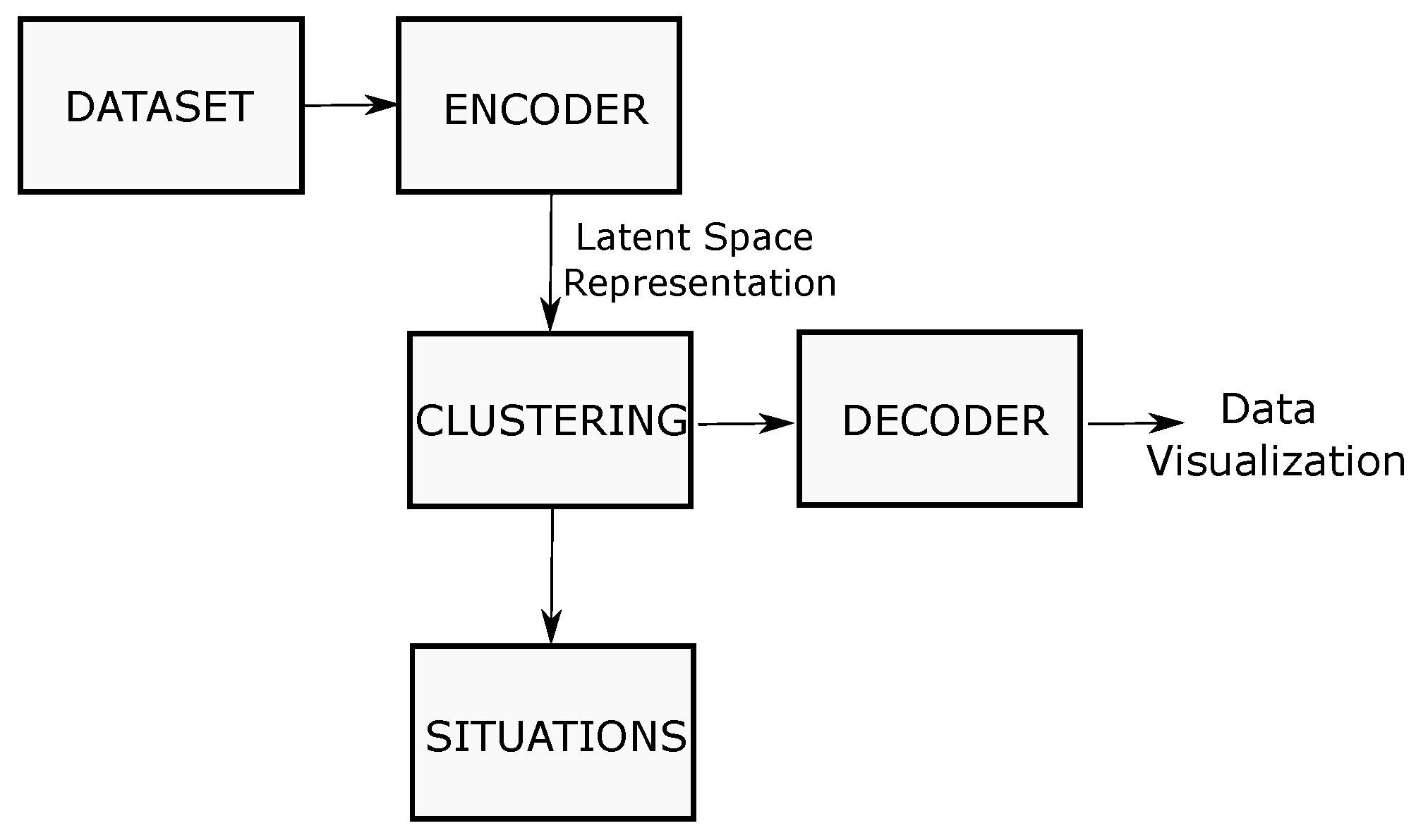
4.1. Driving Situations

This subsection introduces how we create and detect driving situations from observations of the car using a clustering technique to divide a training dataset. Our proposal is to cluster the observations into situations under an unsupervised approach. Unlike previous approaches, we perform the clustering in the latent space of the representations. Given that we are using an unsupervised approach, we require the images from the observations of a previously stored dataset. Next, we apply an encoder (${\Phi }_{\omega }$) to the observations in order to convert those runs into a latent space representation, namely:

$${\Phi }_{\omega }\left(z\right):Z\to L$$

(11)

where L is the latent space. This representation is made up of the main features extracted from the observations. Then, the latent space points are classified using a clustering algorithm. Figure 2 illustrates the clustering methodology. These clusters of similar points are what we call driving situations. In particular, we apply the K-means algorithm for clustering the inputs. The K-means tries to minimize the distance within clusters, i.e.:

$$arg\underset{s}{min}\sum _{i=1}^k\sum _{l\in {\Phi }_{\omega }\left(S_i\right)}{∥l-{\mu }_i∥}^2$$

(12)

where l is the latent space representation of an observation.

K-means requires as input the number of target clusters; however, in our problem, we want to automatically detect the number of situations. To address this issue, we perform an elbow [29] and silhouette analysis [30] to determine the number of clusters, k. According to the inflection point of the curve conformed between the number of clusters and the sum of the squared distance between the centroid and each cluster member, we select the adequate number of centroids as the number of driving situations detected. Once we have the corresponding number of driving situations, we take each centroid and make it go through a decoder that allows us to have a reconstructed image that can help us to have an understanding of what features were taken into account to make the clustering of each situation.

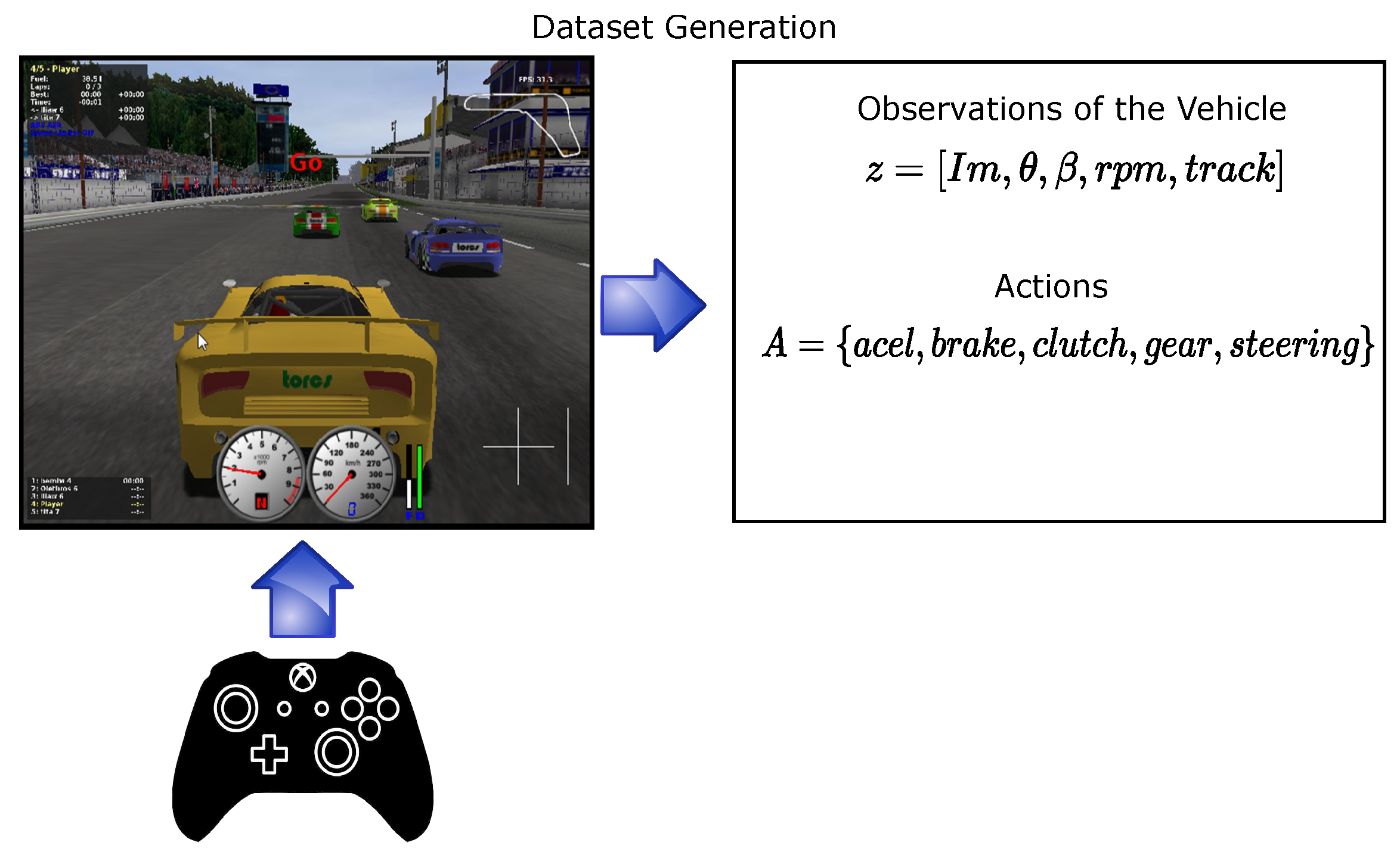
4.1.1. Dataset Collection

The data are generated by a human pilot performing the task of driving. These data were obtained from The Open Racing Car Simulator (TORCS) [31]. The scenarios included in the simulator are restricted to race tracks. In these scenarios, there are neither traffic lights, pedestrians, nor intersections. Simply, eight cars run on the track until three laps are completed. The computer-controlled cars try to overtake each other so that one of them wins. In the case of the human pilot, the objective is to maintain the car running in the lane and not necessarily to win the race. The simulator is open source and includes the dynamic and kinematic model of racing. This simulator is also compatible with ROS [32] m, which is an Operative System for robots and allows us to handle the software and hardware communication.

Formally, the dataset, E, is a collection of tuples conformed by the observations and their corresponding actions of the car:

$$E={\left\{{(z,a)}_t\right\}}_{t=0\dots T}$$

(13)

where T is the amount of tuples.

To create the dataset, the data from the simulator’s sensors was stored, as well as the control inputs (see Figure 3). A total of 14,540 examples were collected from 5 different tracks. Some examples of the scenarios are pictured in Figure 4.

4.1.2. Encoding

The detection of driving situations starts from the image coming from the observations of the car to an autoencoder, the important features of the input data are extracted, and its representation in the latent space is obtained.

We use an autoencoder, ${\Phi }_{\omega }$, based on VGG16 architecture before the flattening and dense layers to obtain the latent space representation of the images. The parameters of the architecture, $\omega$, were pre-trained with ImageNet. Once this is obtained, we conduct K-means on the latent space representation from the encoder to divide the training images into subsets, which we called driving situations (see Figure 5).

The latent space representation of the data helps us learn data characteristics and simplify data representations in order to find patterns with the K-means algorithm easily. In this representation all the features are packed, and all the points from similar data are closer in the space. The latent space representation helps us reduce the dimensionality of the input data and can eliminate non-relevant information. In

Table 3. Dimensionality Reduction of the Input Data.

Data	Size
Input image size	$224\times 224\times 3$
Latent space representation	$7\times 7\times 512$

, we can observe the dimensionality reduction of the input image. This can help us reduce computational consumption and helps avoid overfitting [33,34].

4.1.3. Clustering

The idea of clustering is to minimize the correlation between different clusters and retain more information of input data to accomplish the driving situation classification. Each subset of training images divided by K-means owns minimum distance in the latent space. The purpose of dividing training data is to reduce the loss of information and to improve the performance of each prediction output of the policies.

4.1.4. Defining the Number of Driving Situations

When the sum of the squared distance between the centroid and each cluster member (SSE) is plotted as a function of the number of clusters, notice that SSE decreases as K increases. As more centroids are added, the distance from each point to its closest centroid decreases. There is a good point where the SSE curve begins to bend, defined as the point of maximum curvature in the graph. To estimate this point, we are using the elbow method proposed by Satopaa et al. [29]. To corroborate that this number of clusters is efficient, we combine the elbow method with the silhouette coefficient method (SCM). The SCM is a popular method for measuring the clustering quality [35], which combines both cohesion and separation. The silhouette coefficient is independent from the number of clusters, k. We use both methods to obtain the number of situations. According to each driving situation, we assign a unique driving policy.

4.1.5. Decoder

We use the decoder to reconstruct the data from latent space and form $224\times 224$ pixel size images in RGB format. This helps us to have a reconstructed image of the centroids of each driving situation, and each image helps us try to understand the general driving situations from the dataset. The decoder was implemented as the encoder presented previously but in reverse order.

4.2. Driving Policy Creation

According to the different clusters that we obtain, we divide the representation of the observation into subsets that can be viewed as different driving situations. These subsets contain different relevant information from the input images, but the idea is that only the main features are in the latent space representation, and with this compressed representation, we can improve the training of individual policies. Afterward, each driving policy can learn from each cluster independently and efficiently. These individual policies are learned more quickly compared to a global driving policy, as in the case of the end-to-end systems.

For the training of each driving policy (individual and global), we propose a Deep Neural Network which tries to mimic the behavior of a human pilot using the behavioral cloning technique. The input to the Neural Network is a fixed size $7\times 7\times 512$ from the latent space representation. The representation is passed through a stack of two convolutional layers with kernel $3\times 3$. Then, the data are flattened and passed through a two-layer Fully Connected network. All hidden layers are equipped with the rectification non-linearity (ReLU), and finally, the output is a vector that contains the value of the actions to be performed by the autonomous car (See Figure 6).

The output of the neural network consists of a vector conformed by a tuple of five elements, corresponding to the actions that the car executes to drive. The vector is composed of the values of $[accelerator,brake,clutch,gear,steering]$.

5. Experiments

The first phase of the experiments consists of obtaining the number of situations automatically from our dataset, and the second phase consists of comparing the performance of a global driving policy versus small driving policies corresponding to each driving situation. We train our algorithm using TensorFlow and the KERAS Framework on a laptop with an i7-7700HQ CPU and an NVIDIA GeForce GTX 1070 GPU.

5.1. Data Clustering

We encode all the images using the proposed Neural Network Autoencoder in order to obtain the latent space representation from each image. Using this representation, the driving situations will be obtained using the K-means algorithm.

To select the number of driving situations, we first run the K-means algorithm to obtain between 2 and 39 clusters. We calculate the SSE between the centroid and each cluster member, and it is plotted as a function of the number of clusters (see Figure 7). This give us a general view of the behavior of the SSE and the average silhouette. After that, we focus the analysis in the range of 2 to 20 clusters. This is because, after 20 clusters, the silhouette coefficient diverges from the SSE (see Figure 8).

We use the elbow method to obtain the curve’s point of inflection and use it as the number of situations. Generally, a higher average silhouette coefficient indicates better clustering quality. In this view, the optimal clustering number of grid cells in the study area should be 2, at which the value of the average silhouette coefficient is highest. However, the SSE of this clustering solution ($k=2$) is too large. At $k=7$, the SSE is much lower; according to the elbow method, this is the best k. In addition, the value of the average silhouette coefficient at $k=7$ is also locally high. Therefore, we decided to use it as a number of driving situations detected. In this case, we obtain a total of seven driving situations.

Visualization of the Data Using t-SNE and the Decoder Output

To visualize the obtained data according to each driving situation, we use T-distributed Stochastic Neighbor Embedding (t-SNE). This algorithm allows us to transform high-dimensionality spatial representations as in the case of our latent space representation of the data and let us have a 2D representation, and each situation is colored accordingly, as shown in Figure 9. In general, we can see that most of the situations are clustered correctly in a 2D representation. Although some situations appear uncoupled, we assume that this may be due to the loss of information produced by the dimensional reduction of this plot.

The number of data division examples of our dataset by each driving situation is presented in

Table 4. Dataset division according to each driving situation.

Situation	Number of Examples
Situation 1	2863
Situation 2	3097
Situation 3	1918
Situation 4	1767
Situation 5	1279
Situation 6	1367
Situation 7	2250

. These data clustering results, according to the driving situations, cannot be compared in an objective manner until we use it to train the policies individually and compare the results against a global driving policy.

5.2. Global Driving Policy vs. Driving Situation Policies

The experiment consists of comparing the performance of dividing the problem into driving policies automatically versus a global driving policy, as in the case of end-to-end systems. To accomplish this, we use the complete dataset of 14,540 examples to make the global driving policy learn. The data are divided into 90 percent for training and 10 percent for validation, while, to obtain the automatic policies, the data will be divided as in the proposed methodology. Once both are trained, we will compare the obtained results using the R2 score metric.

First, a Neural Network was trained to have as input the representation in the latent space of the image of the car state, and as output the prediction of the vector of actions that should be applied in order to have a driving policy.

Individual Neural Networks were trained according to the driving situations, and the data were divided according to the clustering of driving situations presented previously. The input normalization is important in most learning algorithms. Since different features might have totally different scales, we use min–max normalization.

The architectures for the end-to-end system and for the individual situation policies are the same in order to compare the obtained results. In

Table 5. Hyperparameters.

Hyperparameter	Value
Input Size	$7\times 7\times 512$
Activation Function	ReLU
Optimizer	ADAM
Learning Rate	0.001
Loss Function	MSE
Epochs	100

, you can see the hyperparameters of the Neural Networks.

It is worth mentioning that no one has used our data for autonomous driving in the state-of-the-art literature. To compare our method with the state-of-the-art methods, we reproduce two different architectures and we train them with our data. The architectures PilotNet and AutoPilot are based on the paper presented by Nvidia [36]. The results are presented in

Table 6. Comparison of the proposed method versus end-to-end methods. The best results are remarked in bold font.

Driving Policy	${\mathit{R}}^2$ Score	MSE
End-to-end	0.33626	0.05766
PilotNet	−0.12808	0.05310
AutoPilot	0.22819	0.05117
Our Policy Division	0.53147	0.00897

. To train these methods, we use the following hyperparameters: activation function: ReLU; Optimizer: Adam; Loss Function: MSE; Epochs = 100; and learning rate = 0.001.

In order to compare the results of the control predictions of the neural networks, the coefficient of determination was used, which tells us how good a regression model is according to the proportion of variability explained by the fitted model [37]:

$$R^2=1-\frac{SSE}{SST}$$

(14)

where: $R^2$ is the coefficient of determination; $SSE$ is the error sum of squares:

$$SSE=\sum _{i=1}^n{(y_i-{\widehat{y}}_i)}^2;$$

(15)

$SST$ is the total corrected sum of squares:

$$SST=\sum _{i=1}^n{(y_i-{\overline{y}}_i)}^2.$$

(16)

Policies Training

Experimental results show that with a fixed number of iterations, this approach achieves better performance compared with an end-to-end system and can converge faster.

The calculated $R^2$ score corresponds to the mean of the five elements of the output vector, which means that every value of the output vector was compared with the ground truth value. Afterwards, the $R^2$ score is averaged to obtain a single value of this metric. In Figure 10, we can see an example of the behavior of the curve during the training of the neural network for a single driving policy.

In Table 6, we can see the result of the end-to-end system, and in

Table 7. Results Obtained From the Driving Situations Policies.

Policy	${\mathit{R}}^2$ Score	MSE
Policy 1	0.62678	0.00598
Policy 2	0.60072	0.00740
Policy 3	0.68023	0.00325
Policy 4	0.62420	0.00516
Policy 5	0.61522	0.00658
Policy 6	0.27024	0.01942
Policy 7	0.30292	0.01505

, we can see the results for each individual driving policy. The mean of $R^2$ Score of all the driving policies was $0.53147$, which is higher than the $0.3362$ obtained from the end-to-end system. For this reason, it is better to divide a global policy into small ones. The individual policies present a better $R^2$ score, which determines that it learns better. Our results show that our method outperforms the tested end-to-end approaches in terms of a bigger R square metric (0.19 over the tested method) and lower mean squared error (0.048 below the tested method).

6. Conclusions

This approach, which applies the “divide and conquer” technique, is more effective than an end-to-end system. This is proven by the $R^2$ score metric; in addition, this methodology helps to identify easily, in the case of a failure, in which policy the problem has occurred, helping us to know whether the reason is a lack of data for this policy so that we could complete the gathering of the data if necessary. Another improvement is that our method helps identify which driving situations are not equally sampled to try to give them priority during training, and it is helpful to divide the policies in an objective way by the K-means distance and not by subjective criteria. The learned policies are valid to apply to the roads where the dataset was obtained. Nevertheless, the method presented in this paper can serve as a step towards developing policies from raw data in other schemes that have the same properties.

In addition, we have found that estimating the situation with a single camera frame and sensor reading is a limited approach because the detected situation can vary rapidly between continuous frames. Therefore, in future work, we will include context and temporal information. Finally, this approach will be tested soon on a real platform.

References

1. Van, N.D.; Sualeh, M.; Kim, D.; Kim, G.W. A hierarchical control system for autonomous driving towards urban challenges. Appl. Sci. 2020, 10, 3543. [Google Scholar] [CrossRef]
2. Badue, C.; Guidolini, R.; Carneiro, R.V.; Azevedo, P.; Cardoso, V.B.; Forechi, A.; Jesus, L.; Berriel, R.; Paixao, T.M.; Mutz, F.; et al. Self-driving cars: A survey. Expert Syst. Appl. 2021, 165, 113816. [Google Scholar] [CrossRef]
3. Buehler, M.; Iagnemma, K.; Singh, S. The DARPA Urban Challenge: Autonomous Vehicles in City Traffic; Springer: Berlin/Heidelberg, Germany, 2009; Volume 56. [Google Scholar]
4. Jo, K.; Kim, J.; Kim, D.; Jang, C.; Sunwoo, M. Development of autonomous car—Part II: A case study on the implementation of an autonomous driving system based on distributed architecture. IEEE Trans. Ind. Electron. 2015, 62, 5119–5132. [Google Scholar] [CrossRef]
5. Galceran, E.; Cunningham, A.G.; Eustice, R.M.; Olson, E. Multipolicy decision-making for autonomous driving via changepoint-based behavior prediction: Theory and experiment. Auton. Robot. 2017, 41, 1367–1382. [Google Scholar] [CrossRef]
6. Somani, A.; Ye, N.; Hsu, D.; Lee, W.S. DESPOT: Online POMDP planning with regularization. Adv. Neural Inf. Process. Syst. 2013, 26, 1772–1780. [Google Scholar]
7. Bandyopadhyay, T.; Won, K.S.; Frazzoli, E.; Hsu, D.; Lee, W.S.; Rus, D. Intention-aware motion planning. In Algorithmic Foundations of Robotics X; Springer: Berlin/Heidelberg, Germany, 2013; pp. 475–491. [Google Scholar]
8. Brechtel, S.; Gindele, T.; Dillmann, R. Probabilistic decision-making under uncertainty for autonomous driving using continuous POMDPs. In Proceedings of the 17th international IEEE Conference on Intelligent Transportation Systems (ITSC), Qingdao, China, 8–11 October 2014; pp. 392–399. [Google Scholar]
9. LeCun, Y.; Bengio, Y.; Hinton, G. Deep learning. Nature 2015, 521, 436–444. [Google Scholar] [CrossRef] [PubMed]
10. Goodfellow, I.; Bengio, Y.; Courville, A. Deep Learning; MIT Press: Cambridge, MA, USA, 2016. [Google Scholar]
11. Rodríguez-Hernandez, E.; Vasquez-Gomez, J.I.; Herrera-Lozada, J.C. Flying through gates using a behavioral cloning approach. In Proceedings of the 2019 International Conference on Unmanned Aircraft Systems (ICUAS), Atlanta, GA, USA, 11–14 June 2019; pp. 1353–1358. [Google Scholar]
12. Farag, W.; Saleh, Z. Behavior cloning for autonomous driving using convolutional neural networks. In Proceedings of the 2018 International Conference on Innovation and Intelligence for Informatics, Computing, and Technologies (3ICT), Sakhier, Bahrain, 18–20 November 2018; pp. 1–7. [Google Scholar]
13. Ly, A.O.; Akhloufi, M. Learning to drive by imitation: An overview of deep behavior cloning methods. IEEE Trans. Intell. Veh. 2020, 6, 195–209. [Google Scholar] [CrossRef]
14. Sharma, S.; Tewolde, G.; Kwon, J. Behavioral cloning for lateral motion control of autonomous vehicles using deep learning. In Proceedings of the 2018 IEEE International Conference on Electro/Information Technology (EIT), Rochester, MI, USA, 3–5 May 2018; pp. 0228–0233. [Google Scholar]
15. Chen, C.; Seff, A.; Kornhauser, A.; Xiao, J. Deepdriving: Learning affordance for direct perception in autonomous driving. In Proceedings of the IEEE International Conference on Computer Vision, Santiago, Chile, 7–13 December 2015; pp. 2722–2730. [Google Scholar]
16. Roy, A.M.; Bose, R.; Bhaduri, J. A fast accurate fine-grain object detection model based on YOLOv4 deep neural network. Neural Comput. Appl. 2022, 34, 3895–3921. [Google Scholar] [CrossRef]
17. Roy, A.M.; Bhaduri, J. Real-time growth stage detection model for high degree of occultation using DenseNet-fused YOLOv4. Comput. Electron. Agric. 2022, 193, 106694. [Google Scholar] [CrossRef]
18. Okumura, B.; James, M.R.; Kanzawa, Y.; Derry, M.; Sakai, K.; Nishi, T.; Prokhorov, D. Challenges in perception and decision making for intelligent automotive vehicles: A case study. IEEE Trans. Intell. Veh. 2016, 1, 20–32. [Google Scholar] [CrossRef]
19. Mihály, A.; Farkas, Z.; Gáspár, P. Multicriteria Autonomous Vehicle Control at Non-Signalized Intersections. Appl. Sci. 2020, 10, 7161. [Google Scholar] [CrossRef]
20. Aeberhard, M.; Rauch, S.; Bahram, M.; Tanzmeister, G.; Thomas, J.; Pilat, Y.; Homm, F.; Huber, W.; Kaempchen, N. Experience, results and lessons learned from automated driving on Germany’s highways. IEEE Intell. Transp. Syst. Mag. 2015, 7, 42–57. [Google Scholar] [CrossRef]
21. Burgard, W.; Fox, D.; Thrun, S. Probabilistic Robotics; MIT Press: Cambridge, MA, USA, 2005; Volume 1. [Google Scholar]
22. Ulbrich, S.; Maurer, M. Probabilistic online POMDP decision making for lane changes in fully automated driving. In Proceedings of the 16th International IEEE Conference on Intelligent Transportation Systems (ITSC 2013), The Hague, The Netherlands, 6–9 October 2013; pp. 2063–2067. [Google Scholar]
23. Zhou, Z.; Zhong, Y.; Liu, X.; Li, Q.; Han, S. DC-MMD-GAN: A New Maximum Mean Discrepancy Generative Adversarial Network Using Divide and Conquer. Appl. Sci. 2020, 10, 6405. [Google Scholar] [CrossRef]
24. Ratner, E.; Hadfield-Menell, D.; Dragan, A.D. Simplifying reward design through divide-and-conquer. arXiv 2018, arXiv:1806.02501. [Google Scholar]
25. Wang, L.; Zhang, J.; Wang, O.; Lin, Z.; Lu, H. Sdc-depth: Semantic divide-and-conquer network for monocular depth estimation. In Proceedings of the IEEE/CVF Conference on Computer Vision and Pattern Recognition, Seattle, WA, USA, 13–19 June 2020; pp. 541–550. [Google Scholar]
26. Kim, J.; Moon, J.; Ryu, J.; Lee, G. Bioinspired Divide-and-Conquer Design Methodology for a Multifunctional Contour of a Curved Lever. Appl. Sci. 2021, 11, 6015. [Google Scholar] [CrossRef]
27. Singh, S.; Jaakkola, T.; Littman, M.L.; Szepesvári, C. Convergence results for single-step on-policy reinforcement-learning algorithms. Mach. Learn. 2000, 38, 287–308. [Google Scholar] [CrossRef] [Green Version]
28. Munos, R.; Stepleton, T.; Harutyunyan, A.; Bellemare, M.G. Safe and efficient off-policy reinforcement learning. arXiv 2016, arXiv:1606.02647. [Google Scholar]
29. Satopaa, V.; Albrecht, J.; Irwin, D.; Raghavan, B. Finding a “kneedle” in a haystack: Detecting knee points in system behavior. In Proceedings of the 2011 31st International Conference on Distributed Computing Systems Workshops, Minneapolis, MN, USA, 20–24 June 2011; pp. 166–171. [Google Scholar]
30. Rousseeuw, P.J. Silhouettes: A graphical aid to the interpretation and validation of cluster analysis. J. Comput. Appl. Math. 1987, 20, 53–65. [Google Scholar] [CrossRef] [Green Version]
31. Wymann, B.; Espié, E.; Guionneau, C.; Dimitrakakis, C.; Coulom, R.; Sumner, A. Torcs, the Open Racing Car Simulator. Software. 2000. Available online: http://torcs.sourceforge.net (accessed on 4 February 2022).
32. Koubâa, A. Robot Operating System (ROS); Springer: Berlin/Heidelberg, Germany, 2017; Volume 1. [Google Scholar]
33. Xie, P.; Deng, Y.; Zhou, Y.; Kumar, A.; Yu, Y.; Zou, J.; Xing, E.P. Learning latent space models with angular constraints. In Proceedings of the International Conference on Machine Learning, PMLR, Sunday, August, 6–11 August 2017; pp. 3799–3810. [Google Scholar]
34. Yaguchi, Y.; Shiratani, F.; Iwaki, H. Mixfeat: Mix feature in latent space learns discriminative space. In Proceedings of the International Conference on Learning Representations, New Orleans, LA, USA, 6–9 May 2019. [Google Scholar]
35. Shi, W.; Zeng, W. Genetic k-means clustering approach for mapping human vulnerability to chemical hazards in the industrialized city: A case study of Shanghai, China. Int. J. Environ. Res. Public Health 2013, 10, 2578–2595. [Google Scholar] [CrossRef]
36. Bojarski, M.; Del Testa, D.; Dworakowski, D.; Firner, B.; Flepp, B.; Goyal, P.; Jackel, L.D.; Monfort, M.; Muller, U.; Zhang, J.; et al. End to end learning for self-driving cars. arXiv 2016, arXiv:1604.07316. [Google Scholar]
37. Walpole, R.E.; Myers, R.H.; Myers, S.L.; Ye, K. Probability and Statistics for Engineers and Scientists; Macmillan: New York, NY, USA, 1993; Volume 5. [Google Scholar]
Figure 1. General overview of a behavior selector system that uses the created policies. First, an input image is converted into its latent space representation, and after that, a situation selector classifies these data into driving situations in which each one of them corresponds to a unique driving policy. Every driving policy outputs the necessary actions which correspond to the steering, accelerator, and brake values.
Applsci 12 03635 g001
Figure 2. Workflow of the unsupervised methodology to automatically classify the situations.
Applsci 12 03635 g002
Figure 3. Using TORCS simulator with ROS compatibility to obtain the data from a human pilot.
Applsci 12 03635 g003
Figure 4. Examples of traffic scenarios from the five different tracks contained in our dataset.
Applsci 12 03635 g004
Figure 5. The architecture of the network in charge of obtaining the latent space representation of the images. The size of the input image is 224 × 224 × 3 and it is reduced to 7 × 7 × 512 .
Applsci 12 03635 g005
Figure 6. The architecture of the policies is a convolutional neural network. The input to the Neural Network is a fixed size 7 × 7 × 512 from the latent space representation. The output is a vector composed of the values of [ a c c e l e r a t o r , b r a k e , c l u t c h , g e a r , a n d s t e e r i n g ] .
Applsci 12 03635 g006
Figure 7. Graph of the SSE and Coefficient Silhouette vs. Number of clusters. We observe that the average silhouette diverges from the SSE curve after 20 clusters.
Applsci 12 03635 g007
Figure 8. Graph of the SSE vs. Number of clusters. The point of inflection of the curve is at 7 according to the elbow method and in combination with the silhouette method.
Applsci 12 03635 g008
Figure 9. Two-dimensional representation of the embedding using t-SNE and color according to each situation. The number assigned to each color corresponds to the driving situation.
Applsci 12 03635 g009
Figure 10. Example of the training of a driving policy. We can appreciate that the training and test curve are decreasing and not diverging.
Applsci 12 03635 g010