Proposing a Method Reducing UGR Calculations for LED Luminaires with Diffusers in Indoor Applications

Featured Application

Proposing a method reducing UGR calculations for LED luminaires with diffuser (uniform luminous intensity distribution).

Abstract

This paper studies discomfort glare in indoor LED lighting systems and proposes a method reducing UGR calculations. There are several methods for expressing discomfort glare, among which the unified glare rating (UGR) method is one of the most popular. It is safe to indicate that the UGR method was introduced before LED lighting became popular in indoor applications. Thus, the UGR method is not versatile currently. In this paper, key limitations of the UGR method are discussed. A method for reducing UGR calculations based on UGR tables for both LED luminaires with diffusers (uniform luminous intensity distribution) and with lenses is proposed. The method is mathematically discussed and its applicability for luminaires is discussed. Also, the luminaires are put through a test and the results from the tests are presented and the feasibility of the method separately from mathematical proofs is examined. The proof and case studies both indicate that the method can be used accurately for luminaires with diffusers. They also illustrate that the accuracy of applying the proposed method to the LED luminaires with lenses is not satisfactory. Simulations are carried out using DIALux lighting design software.

1. Introduction

1.1. LEDs as Low-Energy Indoor Light Sources

In 2015, the International Energy Agency (IEA) reported that 14% of residential electrical energy consumption in Organisation for Economic Co-operation and Development (OECD) countries was related to lighting. For non-OECD countries, the consumption share is usually higher [1]. However, in 2021, the lighting share in building energy consumption became 5% and continues to decrease as a result of measures such as using LEDs instead of less energy-efficient bulbs [2] and electrification of heating systems [3]. The use of LEDs in lighting systems is the result of the energy performance of buildings directive (EPBD)’s nearly zero-energy concept for European countries, which other countries have also adopted [1]. Despite the mentioned decrease in energy consumption share, the absolute amount of energy consumption by lighting continues to increase [3]. This indicates the increasing use of lighting around the world.

During the last decades, various energy initiatives have been undertaken. The use of incandescent lamps is discouraged. Energy-efficient light sources such as light-emitting diodes (LED) and organic light-emitting diodes (OLED) have been introduced. The EU has published “Lighting the Future—Accelerating the deployment of Innovative Lighting Technologies”, proposing to apply policy innovations in Europe for the pervasive use of solid-state lighting products. The mentioned products will play a significant role in energy saving in the near future [1,4].

The efficacy of LEDs can reach 200 lm/W. Thus, these light sources are very attractive and are regarded as energy-efficient light sources [5]. However, LEDs are relatively small and compact light sources, which can deliver very high luminous intensity, resulting in significant discomfort glare. Dealing with these high intensities is an ongoing challenge faced by many manufacturers of luminaires.

Discomfort glare can be expressed numerically by the unified glare rating UGR, which was first adopted to lighting standards in 1995. Over the years, the UGR has been applied as a primary and common metric for quantifying discomfort glare [6,7].

This paper discusses challenges related to the use of the UGR evaluation method, especially in modern LED lighting systems, and proposes a novel method for reducing UGR calculations.

1.2. Glare Evaluation by UGR

UGR is a glare quantification tool which is based on contrast noticeable by an observer. Figure 1 shows an example of a space with highly contrasting LED luminaires.

For an indoor observer, the UGR formula is given as [8]:

$$UGR=8\log \left[\frac{0.25}{L_b}{\displaystyle \sum }_{i=1}^n\frac{L_i^2{\omega }_i}{p_i^2}\right]$$

(1)

where $L_b$ is the background luminance in cd/m², $L_i$ is the luminance of the luminaire in cd/m², ${\omega }_i$ is the solid angle of the luminaire in sr, $p_i$ is the Guth position index of the luminaire, and n is the number of luminaires in the observer’s field of view.

Assumptions and limitations of the UGR method:

• UGR cannot be applied for completely indirect lighting systems or luminous ceilings [8].
• UGR is not applicable for point sources [8,9].
• UGR cannot be computed for very thin beam patterns pointing straight down [4,7,9,10].
• It is assumed the room walls are uniformly illuminated [8].
• UGR is unreliable for luminaires with non-uniform luminous intensity distributions [9,11].

Alongside the mentioned limitations, discomfort glare evaluation is a challenging effort. Quek et al. said that the two categories of effects which lead to discomfort glare are saturation and contrast. UGR is only based on contrast effect. The performance of metrics using contrast effect is poor in brighter scenes. Quek et al. also stated that applicability of metrics using two or more effects simultaneously is limited by their dataset development scope [12]. Fotios and Kent argue that in experiments, biases can affect reliability and validity of data. They indicate that among four psychological procedures used for explicit quantitative measurement, adjustment and category are the most prevalent procedures in discomfort glare evaluation. The two mentioned procedures are subjected to biases such as stimulus range, anchor, and order effect biases [13]. Consequently, UGR as a metric which developed using adjustment procedure [14] is subjected to the mentioned biases. Pierson et al. suggested that there is possibility of the existence of some unknown psychological and physiological factors influencing discomfort glare perception. They also noted that the intensity of each influencing factor cannot be understood and explained accurately. Therefore, an exact correlation between discomfort glare as assessed by the metrics and as perceived by subjects cannot be expected. They also, based on previous research, reported that even age and culture have effects on discomfort glare [15]. Wienold et al. based on investigating 22 glare prediction metrics, stated that still there is not a reliable metric that considers all scenarios [16]. Słomiński obtained UGR for bare and diffuser-covered LED luminaires. UGR was calculated using both luminance measured by an image luminance measuring device (ILMD) and luminous intensity numbers in the luminaire IES file. The results showed for both luminaires that the UGRs calculated by the two methods have substantial differences. He recommended correct luminance distribution measurement according to human eye geometry and adding a factor to the UGR formula related to luminaire construction, particularly for luminaires with non-uniform luminance distribution on the whole surface [9].

According to limitations of the existing UGR method as pointed out above, alternatives such as the model based on receptive fields introduced in [17] are proposed. The model better interprets visual discomfort, especially in the case of luminaires with non-uniform luminous intensity distribution. However, the model still must be improved for indirect viewing angles and different background luminance levels. As mentioned previously, UGR is a widely accepted standard visual discomfort rating index, but according to limitations, researchers are working to enhance its applicability [10]. T. Porsch et al. [18] introduced software for automated UGR calculation using imaging luminance measuring devices (ILMDs). In [19], evaluations were made by comparing UGRs obtained with the original method. In this research, the luminaires with non-uniform luminous intensity distribution were divided into smaller subdivisions. The results showed that UGR was not robust for luminaires with non-uniform luminous intensity distribution glare evaluation. Therefore, it is necessary to perform further research to find a robust method for glare evaluation for both luminaires with uniform and non-uniform luminous intensity distribution. Scheir et al. [20] defined an improved UGR standard method which took into account pixels of a luminaire with luminance above a threshold as the luminating part. The other pixels were considered as background luminance. The method can better describe the glare felt by observers than the standard CIE-proposed UGR calculation method. In [21], UGR for conventional fluorescent luminaires was obtained by three methods using DIALux software, LMK software, and a Python-based software. UGR was calculated by the mentioned methods for the same spaces. The results’ similarity showed the applicability of UGR for luminaires with uniform luminous intensity distribution such as the fluorescent luminaires. Tyukhova et al. [22] used the UGR method for small sources to address glare produced by some types of LED sources via combining measurement and software analysis. Their study did not address LED luminaires with multiple light sources (LED matrix) or when several light sources were present in the field of view simultaneously. Sharma et al. [23] demonstrated the importance of light source positioning for controlling UGR. Additionally, they showed the correlation between UGR and observers’ visual discomfort perception by simultaneously using a qualitative method. Wolska and Sawicki suggested a procedure for using high dynamic range imaging (HDRI) techniques for UGR assessment by determining the best exposure time. Their method uses ILMD. Consequently, their proposed procedure requires the use of technical devices [6].

The mentioned studies showed that, despite limitations of the UGR method in some conditions as explained previously, research to improve UGR to cope with different scenarios and conditions, especially modern luminaires such as LEDs, is plentiful. Proposed methods for UGR calculation improvement did not address reducing the number of calculations for obtaining UGR.

The reduction and simplification of the calculations and models have received attention in science fields as can be seen in [24,25,26,27]. Due to the prevalence of UGR application, it is useful to devise methods for decreasing the number of UGR calculations.

The proposed tabular method makes it possible to decrease UGR calculations by using the UGR table and shows the UGR table’s applicability for points inside a room which the table was not originally designed for.

1.3. Paper Structure

In this paper, we investigate whether approaches and methods with fewer calculations can be proposed for UGR calculation for different LED luminaire types. In Section 2, the proposed tabular method for UGR calculation for LED luminaires is introduced. Then, the feasibility of the method is proved. Afterwards, the method is verified by comparing the method’s results with those obtained from the simulation. Finally, in Section 3, the UGR calculation method proposed in this paper and its validity are summarized and presented in brief, while future research areas in the field are suggested.

2. Tabular Method for Reducing UGR Calculations, for Every Point on the Room Midline

2.1. Introduction to the Method

UGR calculation for points inside an indoor space in lighting design is essential. Since, as stated in AS/NZS 1680, not only criteria such as minimum needed work-plane illuminance for a particular task should be met, but also UGR criterion observation for users’ visual comfort is mandatory [28]. By referring to Equation (1), it can be deduced that UGR calculation for a large number of luminaires in a room requires a high number of calculations. The reason is the number of summands in front of the sigma operator, which is equivalent to the number of luminaires. An approach that drastically reduces the calculation number can proportionally reduce the time and energy consumption for UGR calculation.

According to CIE 117-1995 [8], UGR tables are provided by luminaires’ manufacturers. This table is designed as a very useful and efficient tool for fast estimation and calculation of glare only at the midpoints of the room’s walls. A sample of a UGR table is illustrated in Table S1 in the Supplementary File. By finding the desired X and Y dimensions, the corresponding luminaire direction, and the surface’s reflection factor, the UGR can be obtained.

Where intended number exists in the table, it can be used directly, and in case of not existence, simple interpolation (extrapolation) using numbers in the UGR table can be used as a tool to estimate UGR. (All interpolations (extrapolations) used in this research are well-known linear (1D) [29] (for 2 known points) or bilinear (2D) [30] (for 4 known points) interpolations (extrapolations).)

Through theoretical and experimental investigations in this paper, it is proved that in addition to the points in the room for which the UGR table is designed, this table can be used for all points on the room’s midlines to obtain the UGR (Figure 2).

A method for using numbers in the UGR table for obtaining UGR on the room’s midlines is proposed. In the proposed method, by simply using numbers in the UGR table issued by luminaires’ manufacturer, we attempt to obtain UGR for every point on the room’s midlines. The proposed method is fast because, as mentioned previously, for a room with dimension $\mathrm{XH}\times \mathrm{YH}$, for the very first points of the observer’s movement path, the number of summands in front of the sigma operator in Equation (1) is $n=\mathrm{X}\times \mathrm{Y}$ (number of luminaires in front of the observer). However, in the proposed method, only one 2D interpolation or extrapolation between related adjacent numbers of the table is required.

2.2. Method Explanation

When an observer is located at a point with a certain distance from the walls, it is rational to have an estimation for UGR at that point. Reducing the number of calculations of Equation (1) for that point would be desirable for reducing UGR calculation time and energy.

A UGR table is a table as illustrated in Supplementary Table S1. As mentioned before, it is designed for obtaining UGR in the middle of each wall in a room. In the proposed method, when a point on a room midline is considered, for obtaining UGR for observer at that point, it is assumed that the space behind the observer is removed and UGR is obtained from the UGR table for a new room with space equal to the remaining space of the main room (The new room dimensions in the observer’s field of view are smaller, but in other directions, dimensions of the main and new rooms are equal) in front of the observer (Figure 3). If the exact corresponding dimensions do not exist in the table, the related UGR can be interpolated or extrapolated.

In this research, the Y direction is assumed to be the direction of the observer’s movement, and the X direction is assumed to be perpendicular to the direction of the observer’s movement.

As previously indicated, for a sample luminaire, the UGR table is illustrated in the Supplementary File as Table S1. If it is assumed the room has dimensions of 8 m × 8 m, then, based on a luminaire height of H = 2 m from the observers’ eye, the length and width dimensions of the room will be 4H × 4H. Reflection factors for the ceiling, walls, and floors are 70, 50, and 20, respectively. Viewing direction is at right angles to the lamp axis. Therefore, for the observer position at the wall midpoint, UGR will be 21.2; for the observer position in the center of the room with the same viewing direction, UGR will be 18.9. The latter number is obtained based on the proposed method and corresponds to a room with dimensions of 8 m × 4 m (4H × 2H), while in reality, the dimensions of the room have not been changed.

2.3. Mathematical and Practical Proof of Feasibility of the Method

As explained previously, in the proposed method, UGR table numbers or their 2D interpolation or extrapolation are used as the UGR for the observer’s position on the room’s midline. Therefore, it is assumed that UGR for an observer at any point on a room’s midline is equal to UGR for an observer in a room with size equal to the space in front of the first observer when the second observer is placed in the middle of one wall looking toward the opposite-side wall in a smaller room. For proving the validity of idea, it should be proved that UGRs obtained for both observers are adequately close to each other.

To start the proof, it is necessary to refer to Equation (1), the well-known CIE 117:1995 formula for UGR calculation [8]. The formula takes into account all but one of the variables which are directly related to the observer’s field of view. Therefore, except for one variable, all variables—$L_i$ as the luminance of the luminaire i, ${\omega }_i$ as the solid angle of the luminaire i, and $p_i$ as the Guth position index of the luminaire i—are directly related to the luminaires which are in the observer’s sight. The only parameter which considers the effect of luminaires out of the observer’s sight is L_b, the background luminance. Therefore, for two mentioned observers in two different rooms, it is enough to prove that the background luminances are close to each other such that when using them in Equation (1), the resulted UGRs are reasonably close to each other.

Consider two mentioned observers. One is in a room in a position which places some of the luminaires in front of them (in their field of view), and some of the luminaires behind them (Figure 4a). The other observer exists in a room containing only the luminaires which are in the first observer’s field of view. The nearest wall behind the second observer is at a distance of H/2 from the first row of the luminaires in front of them (Figure 4b). The arrangement of the luminaires is as the standard arrangement explained in CIE 117:1995 [8].

For UGR calculation in the two rooms illustrated in Figure 4a,b, Equation (1) can be stated as:

$$\begin{array}{l}UG{R}_{main room \left(for observer position\right)}\\ =8\log \left[\frac{0.25}{L_{b_a}}·\left(\frac{L_{1_a}^2{\omega }_{1_a}}{p_{1_a}^2}+\frac{L_{2_a}^2{\omega }_{2_a}}{p_{2_a}^2}+\frac{L_{3_a}^2{\omega }_{3_a}}{p_{3_a}^2}+\cdots \right)\right]\end{array}$$

(2)

$$\begin{array}{l}UG{R}_{\mathit{\text{corresponding smaller room}}\left(\mathit{\text{Observer is located in the middle of one wall}}\right)}\\ =8\log \left[\frac{0.25}{L_{b_b}}·\left(\frac{L_{1_b}^2{\omega }_{1_b}}{p_{1_b}^2}+\frac{L_{2_b}^2{\omega }_{2_b}}{p_{2_b}^2}+\frac{L_{3_b}^2{\omega }_{3_b}}{p_{3_b}^2}+\cdots \right)\right]\end{array}$$

(3)

where the parameters with indices a and b correspond to rooms a and b as illustrated in Figure 4a,b.

It should be proved that:

$$\begin{array}{c}UG{R}_{main room \left(for current observer\text{'}s position\right)}\\ =UG{R}_{corresponded smaller room\left(Observer is located in the middle of one wall\right)}\end{array}$$

(4)

Therefore, from Equations (2)–(4):

$$8\log \left[\frac{0.25}{L_{b_a}}·\left(\frac{L_{1_a}^2{\omega }_{1_a}}{p_{1_a}^2}+\frac{L_{2_a}^2{\omega }_{2_a}}{p_{2_a}^2}+\frac{L_{3_a}^2{\omega }_{3_a}}{p_{3_a}^2}+\cdots \right)\right]=8\text{log}\left[\frac{0.25}{L_{b_b}}·\left(\frac{L_{1_b}^2{\omega }_{1_b}}{p_{1_b}^2}+\frac{L_{2_b}^2{\omega }_{2_b}}{p_{2_b}^2}+\frac{L_{3_b}^2{\omega }_{3_b}}{p_{3_b}^2}+\cdots \right)\right]$$

(5)

Or:

$$\frac{0.25}{L_{b_a}}·\left(\frac{L_{1_a}^2{\omega }_{1_a}}{p_{1_a}^2}+\frac{L_{2_a}^2{\omega }_{2_a}}{p_{2_a}^2}+\frac{L_{3_a}^2{\omega }_{3_a}}{p_{3_a}^2}+\cdots \right)=\frac{0.25}{L_{b_b}}·\left(\frac{L_{1_b}^2{\omega }_{1_b}}{p_{1_b}^2}+\frac{L_{2_b}^2{\omega }_{2_b}}{p_{2_b}^2}+\frac{L_{3_b}^2{\omega }_{3_b}}{p_{3_b}^2}+\cdots \right)$$

(6)

As a result, by proving:

$$L_{i_a}=L_{i_b}$$

(7)

$$w_{i_a}=w_{i_b}$$

(8)

$$p_{i_a}=p_{i_b}$$

(9)

$$L_{b_a}=L_{b_b}$$

(10)

the equality in Equation (6) will be proved.

As can be deduced from Figure 4a,b, since there are same luminaires in both observers’ fields of view in the mentioned figures, Equations (7)–(9) are true.

However, L_b in Equation (1) is the only variable which is not related only to the luminaires in the observer’s field of view. Therefore, the aim is to prove that the values of L_b for both of the rooms and observers’ positions are reasonably close to each other. For this aim, the range of changes in background luminance will be obtained based on observers’ position changes; we also examine whether background luminance change can be ignored.

In this research, the CIE 190:2010 [31] method for L_b calculation will be used:

$$L_b=\frac{E_{WID}}{\pi }$$

(11)

where, E_WID is an indirect component of the illuminance on the wall produced by luminaires. In turn, E_WID is:

$$E_{WID}=\frac{F_{UWID}·N·{\mathsf{\Phi }}_0}{A_W}$$

(12)

where F_UWID is the indirect utilization factor for walls, N is the number of luminaires, A_W is the total area of walls (m²) (W stands for wall) between the reference plane and the luminaires’ installation plane, and Φ₀ equals 1000 lm (reference luminous flux) when the luminaire’s luminous intensity distribution is given in cd per 1000 lm. It should be noted that in case of giving luminous intensity distribution based on luminaire luminous flux, the luminous intensity distribution numbers should be divided by Φ_luminaire/1000 to change the luminous intensity unit to cd per 1000 lm, which makes the use of Equation (12) possible.

As the observer moves toward the opposite-side wall in the main (first) room, the size of the smaller (second) room corresponding to the observer’s position in the first room (In the second room, the observer’s distance from the opposite-side wall is the same as the first observer, but the nearest wall behind the second observer is exactly H/2 distance from the first row of the luminaires in front of them) changes as illustrated in Figure 4a,b, and the length of the second room in the first observer’s path decreases. Meanwhile, the number of luminaires in both observers’ fields of view decreases.

If there is a room with dimensions of XH × Y_LH (the main room) and an observer moves in Y direction, it can be said when the observer in the main room is in the position (Y₀ + ΔY)H (distance from opposite-side wall), and for H = 2 m, the number of luminaires effecting background luminance would be:

$$N=\mathrm{X}\times ({\mathrm{Y}}_{\mathrm{L}})$$

(13)

and the area of wall which reflects background luminance is:

$$A_W=8\left(\mathrm{X}+({\mathrm{Y}}_{\mathrm{L}})\right)$$

(14)

where Y₀ is the smallest distance of the observer from the opposite-side wall, ΔY is added to Y₀ for obtaining the Y corresponding to the observer’s position, and Y_L is the length of the main room (Y and X should be multiplied by H for obtaining dimensions in meters).

For the corresponding smaller room:

$$N=\mathrm{X}\times ({\mathrm{Y}}_0+∆\mathrm{Y})$$

(15)

and

$$A_W=8\left(\mathrm{X}+({\mathrm{Y}}_0+∆\mathrm{Y})\right)$$

(16)

By putting aside A_w, N, and Φ₀, the remaining part of Equation (12) is related to the indirect utilization factor of the walls, which is the next part of the formula to be considered.

Indirect utilization factor for walls is [31]:

$$F_{UWID}=F_{DF}{F}_{T,FW}+F_{DW}\left(F_{T,WW-1}\right)+F_{DC}{F}_{T,CW}$$

(17)

In Equation (17), distribution factors F_DF, F_DW, and F_DC are defined as [31]:

$$F_{DF}={\mathsf{\Phi }}_{ZL}/{\mathsf{\Phi }}_0$$

(18)

$$F_{DW}={\mathrm{R}}_{DLO}-F_{DF}$$

(19)

$$F_{DC}={\mathrm{R}}_{ULO}$$

(20)

F_DF and F_DW are derived from Φ_ZL, which is the sum of the cumulative CIE zonal fluxes multiplied by the geometric factor values for luminaires in the standard array. Geometric factors are related to the room’s dimensions. Therefore, they change in small rooms when the observer’s position changes. However, F_DC is derived from R_ULO, which is only related to the luminaire’s luminous intensity specifications. Then, it is independent of the observer’s position in the room. Based on changing parts of F_UWID as the observer’s position changes, its range of change will be investigated as follows.

Φ_ZL as an important part of F_UWID is expressed as:

$${\mathsf{\Phi }}_{ZL}={\mathsf{\Phi }}_{ZL1}{F}_{GL1}+{\mathsf{\Phi }}_{ZL2}{F}_{GL2}+{\mathsf{\Phi }}_{ZL3}{F}_{GL3}+{\mathsf{\Phi }}_{ZL4}{F}_{GL4}$$

(21)

Φ_ZL1, Φ_ZL2, Φ_ZL3, and Φ_ZL4 are only related to each luminaire’s luminous flux properties and are not related to the observer’s position or the room’s dimensions. Then, they are independent of the observer’s position in the room.

By rewriting F_UWID formula (Equation (17)) considering the change in the observer’s position:

$$\begin{array}{cc}{F}_{UWID}\left({\mathrm{Y}}_0+\mathsf{\Delta }\mathrm{Y}\right)\hfill & =F_{DF}\left({\mathrm{Y}}_0+\mathsf{\Delta }\mathrm{Y}\right)F_{T,FW}\left({\mathrm{Y}}_0+\mathsf{\Delta }\mathrm{Y}\right)\hfill \\ & +F_{DW}\left({\mathrm{Y}}_0+\mathsf{\Delta }\mathrm{Y}\right)F_{T,WW-1}\left({\mathrm{Y}}_0+\mathsf{\Delta }\mathrm{Y}\right)\hfill \\ & +F_{DC}\left({\mathrm{Y}}_0+\mathsf{\Delta }\mathrm{Y}\right)F_{T,CW}\left({\mathrm{Y}}_0+\mathsf{\Delta }\mathrm{Y}\right) \hfill \end{array}$$

(22)

Following that, for finding the changing range for F_UWID, the changing range for the right side of Equation (22) will be investigated in detail.

For F_DF, on the right side of Equation (22), it can be written:

$$\begin{array}{c}{F}_{DF}\left({\mathrm{Y}}_0+\mathsf{\Delta }\mathrm{Y}\right)=\frac{{\mathsf{\Phi }}_{ZL}\left({\mathrm{Y}}_0+\mathsf{\Delta }\mathrm{Y}\right)}{{\mathsf{\Phi }}_0}\\ =\frac{\left({\mathsf{\Phi }}_{ZL1}{F}_{GL1}\left({\mathrm{Y}}_0+\mathsf{\Delta }\mathrm{Y}\right)+{\mathsf{\Phi }}_{ZL2}{F}_{GL2}\left({\mathrm{Y}}_0+\mathsf{\Delta }\mathrm{Y}\right)+{\mathsf{\Phi }}_{ZL3}{F}_{GL3}\left({\mathrm{Y}}_0+\mathsf{\Delta }\mathrm{Y}\right)+{\mathsf{\Phi }}_{ZL4}{F}_{GL4}\left({\mathrm{Y}}_0+\mathsf{\Delta }\mathrm{Y}\right)\right)}{{\mathsf{\Phi }}_0} \end{array}$$

(23)

As previously mentioned, in Equation (23), Φ_ZLns are related to the luminaires’ specifications and do not change when the room’s specifications change. Geometric factors (F_GLns) are related to the room’s dimensions and ranges of their changing with room dimensions are illustrated in

Table 1. Geometric factors changing when room dimensions change for X = 2~12 and Y = 4~8. (The negative numbers show decreasing and the positive numbers show increasing of the geometric factors with increasing Y).

X	Y	ΔYFGL1	ΔYFGL2	ΔYFGL3	ΔYFGL4
2	4~8	−0.062	−0.011	0.079	0.011
4	4~8	−0.058	−0.092	0.015	0.024
8	4~8	−0.041	−0.177	0.191	0.052
12	4~8	−0.032	−0.0209	0.199	0.071

.

From Table 1, it can be understood that when a room’s Y dimension increases, F_GL1 and F_GL2 decrease and F_GL3 and F_GL4 increase. From each row of Table 1 and considering Equation (21), it can be deduced that for luminaires whose Φ_ZLn values are close to each other, the increasing and decreasing of related geometric factors can cancel each other and CIE zonal flux (Φ_ZL) can change little when a room’s dimensions change. Knowing that, and also since in Equation (18), F_DF is CIE zonal flux (Φ_ZL) divided by 1000 lm, F_DF change based on changes in room dimensions is not prominent.

From Equation (19) and keeping in mind that R_DLO is not dependent on room dimensions:

$$F_{DW}={\mathrm{R}}_{DLO}-F_{DF}\Rightarrow {∆}_{\mathrm{Y}}{F}_{DW}={∆}_{\mathrm{Y}}{\mathrm{R}}_{DLO}-{∆}_{\mathrm{Y}}{F}_{DF}\stackrel{{∆}_{\mathrm{Y}}{\mathrm{R}}_{DLO}=0}{\Rightarrow }{∆}_{\mathrm{Y}}{F}_{DW}=-{∆}_{\mathrm{Y}}{F}_{DF}$$

(24)

Consequently, F_DW change which is equal to F_DF change but with a negative sign is not also prominent.

Since luminaires’ R_ULO value is usually negligible, the F_DC also can be assumed to be a negligible value. Therefore, F_DF and F_DW are the only distribution factors influencing the change of the indirect utilization factor of the walls.

Table 2. Transfer factors changing with the changes in a room’s dimensions for X = 2~12 and Y = 4~8. (All changes are in form of decreasing with increasing Y).

X	Y	ΔYFT,FW	ΔYFT,ww−1	ΔYFT,CW
2	4~8	−0.020	−0.044	−0.065
4	4~8	−0.027	−0.054	−0.082
8	4~8	−0.032	−0.056	−0.092
12	4~8	−0.034	−0.057	−0.096

illustrates a range of transfer factors’ change according to the change in a room’s dimensions.

Validity of using data illustrated in Table 1 and Table 2 requires maintaining a trend of change for geometric and transfer factors linearly, both inside and outside of the studied range (X = 2H, 4H, 8H, and 12H, Y = 4H, 6H, and 8H). Therefore, linear regression was applied to trends of mentioned factors for inside and outside of the studied range where data were available, and R²-values of regression for all factors for a common range are illustrated in Tables S3 and S4. Based on data illustrated in Tables S2 and S3, the average of R²-value for linear regression of geometric factors is 0.8701 and for transfer factors is 0.9651. The mentioned R²-values show acceptable linear correlation between room dimension in the Y direction and geometric and transfer factors. It shows the possibility of generalization of the results obtained in the studied dimension range for outside the range.

From Equation (22), the average change of the indirect utilization factor for walls based on the change of distribution and transfer factors can be stated as Equation (25):

$$\begin{array}{cc}\overline{F_{UWID}\left({\mathrm{Y}}_0+\mathsf{\Delta }\mathrm{Y}\right)}\hfill & =\overline{F_{UWID} \left({\mathrm{Y}}_0\right)}+\overline{∆F_{UWID} \left({\mathrm{Y}}_0\right)}\hfill \\ & =(\overline{F_{DF}\left({\mathrm{Y}}_0\right)}+\overline{∆F_{DF}({\mathrm{Y}}_0)})\left(\overline{F_{T,FW}\left({\mathrm{Y}}_0\right)}+\overline{∆F_{T,FW}\left({\mathrm{Y}}_0\right)}\right)\hfill \\ & +\left(\overline{F_{DW}\left({\mathrm{Y}}_0\right)}+\overline{∆F_{DW}\left({\mathrm{Y}}_0\right)}\right)\left(\overline{F_{T,WW-1}\left({\mathrm{Y}}_0\right)}+\overline{∆F_{T,WW-1}\left({\mathrm{Y}}_0\right)}\right)\hfill \\ & +\left(\overline{F_{DC}\left({\mathrm{Y}}_0\right)}+\overline{∆F_{DC}\left({\mathrm{Y}}_0\right)}\right)\left(\overline{F_{T,CW}\left({\mathrm{Y}}_0\right)}+\overline{∆F_{T,CW}\left({\mathrm{Y}}_0\right)}\right)\hfill \end{array}$$

(25)

From Equations (19), (20), and (25):

$$\begin{array}{cc}\overline{F_{UWID}\left({\mathrm{Y}}_0+\mathsf{\Delta }\mathrm{Y}\right)}\hfill & =\left(\overline{F_{DF}\left({\mathrm{Y}}_0\right)}+\overline{∆F_{DF}\left({\mathrm{Y}}_0\right)}\right)\left(\overline{F_{T,FW}\left({\mathrm{Y}}_0\right)}+\overline{∆F_{T,FW}\left({\mathrm{Y}}_0\right)}\right)+(\overline{{\mathrm{R}}_{DLO}}\hfill \\ & -\overline{F_{DF}\left({\mathrm{Y}}_0\right)}-\overline{∆F_{DF}\left({\mathrm{Y}}_0\right)})\left(\overline{F_{T,WW-1}\left({\mathrm{Y}}_0\right)}+\overline{∆F_{T,WW-1}\left({\mathrm{Y}}_0\right)}\right)\hfill \\ & +\left(\overline{R_{ULO}}+\overline{∆R_{ULO}}\right)(\overline{F_{T,CW}\left({\mathrm{Y}}_0\right)}+\overline{\Delta F_{T,CW}\left({\mathrm{Y}}_0\right)})\hfill \end{array}$$

(26)

Since, in many luminaires, luminous intensity in the upper hemisphere is near zero, R_ULO also equals zero. Therefore, Equation (26) would be:

$$\begin{array}{cc}\overline{F_{UWID}\left({\mathrm{Y}}_0+\mathsf{\Delta }\mathrm{Y}\right)}\hfill & =\left(\overline{F_{DF}\left({\mathrm{Y}}_0\right)}+\overline{∆F_{DF}\left({\mathrm{Y}}_0\right)}\right)(\overline{F_{T,FW}\left({\mathrm{Y}}_0\right)}+\overline{∆F_{T,FW}\left({\mathrm{Y}}_0\right)})+(\overline{{\mathrm{R}}_{DLO}}\hfill \\ & -\overline{F_{DF}\left({\mathrm{Y}}_0\right)}-\overline{∆F_{DF}\left({\mathrm{Y}}_0\right)})\left(\overline{F_{T,WW-1}\left({\mathrm{Y}}_0\right)}+\overline{∆F_{T,WW-1}\left({\mathrm{Y}}_0\right)}\right)\hfill \end{array}$$

(27)

By expanding Equation (27):

$$\begin{array}{cc}\overline{F_{UWID}\left({\mathrm{Y}}_0+\mathsf{\Delta }\mathrm{Y}\right)}& =\overline{F_{DF}\left({\mathrm{Y}}_0\right)}·\overline{F_{T,FW}\left({\mathrm{Y}}_0\right)}+\overline{F_{DF}\left({\mathrm{Y}}_0\right)}·\overline{∆F_{T,FW}\left({\mathrm{Y}}_0\right)}+\overline{∆F_{DF}\left({\mathrm{Y}}_0\right)}\hfill \\ & ·\overline{F_{T,FW}\left({\mathrm{Y}}_0\right)}+\overline{∆F_{DF}\left({\mathrm{Y}}_0\right)}·\overline{∆F_{T,FW}\left({\mathrm{Y}}_0\right)}+\overline{{\mathrm{R}}_{DLO}}·\overline{F_{T,WW-1}\left({\mathrm{Y}}_0\right)}\hfill \\ & +\overline{{\mathrm{R}}_{DLO}}·\overline{∆F_{T,WW-1}\left({\mathrm{Y}}_0\right)}-\overline{F_{DF}\left({\mathrm{Y}}_0\right)}·\overline{F_{T,WW-1}\left({\mathrm{Y}}_0\right)}-\overline{F_{DF}\left({\mathrm{Y}}_0\right)}\hfill \\ & ·\overline{∆F_{T,WW-1}\left({\mathrm{Y}}_0\right)}-\overline{∆F_{DF}\left({\mathrm{Y}}_0\right)}·\overline{F_{T,WW-1}\left({\mathrm{Y}}_0\right)}-\overline{∆F_{DF}\left({\mathrm{Y}}_0\right)}\hfill \\ & ·\overline{∆F_{T,WW-1}\left({\mathrm{Y}}_0\right)}\hfill \end{array}$$

(28)

Multiplication of two differential values makes very small values. Therefore, the terms including multiplication of two differential values are removed from Equation (28):

$$\begin{array}{cc}\overline{F_{UWID}\left({\mathrm{Y}}_0+\mathsf{\Delta }\mathrm{Y}\right)}& =\overline{F_{DF}\left({\mathrm{Y}}_0\right)}·\overline{F_{T,FW}\left({\mathrm{Y}}_0\right)}+\overline{F_{DF}\left({\mathrm{Y}}_0\right)}·\overline{∆F_{T,FW}\left({\mathrm{Y}}_0\right)}+\overline{∆F_{DF}\left({\mathrm{Y}}_0\right)}\hfill \\ & ·\overline{F_{T,FW}\left({\mathrm{Y}}_0\right)}+\overline{{\mathrm{R}}_{DLO}}·\overline{F_{T,WW-1}\left({\mathrm{Y}}_0\right)}+\overline{{\mathrm{R}}_{DLO}}·\overline{∆F_{T,WW-1}\left({\mathrm{Y}}_0\right)}\hfill \\ & -\overline{F_{DF}\left({\mathrm{Y}}_0\right)}·\overline{F_{T,WW-1}\left({\mathrm{Y}}_0\right)}-\overline{F_{DF}\left({\mathrm{Y}}_0\right)}·\overline{∆F_{T,WW-1}\left({\mathrm{Y}}_0\right)}-\overline{∆F_{DF}\left({\mathrm{Y}}_0\right)}\hfill \\ & ·\overline{F_{T,WW-1}\left({\mathrm{Y}}_0\right)}\hfill \end{array}$$

(29)

By subtracting F_UWID(Y₀) obtained by Equation (17) from F_UWID(Y₀+ΔY) in Equation (29):

$$\begin{array}{cc}\overline{F_{UWID}\left({\mathrm{Y}}_0+\mathsf{\Delta }\mathrm{Y}\right)}& -\overline{F_{UWID}\left({\mathrm{Y}}_0\right)}\hfill \\ & =\overline{F_{DF}\left({\mathrm{Y}}_0\right)}·\overline{∆F_{T,FW}\left({\mathrm{Y}}_0\right)}+\overline{∆F_{DF}\left({\mathrm{Y}}_0\right)}·\overline{F_{T,FW}\left({\mathrm{Y}}_0\right)}+\overline{{\mathrm{R}}_{DLO}}\hfill \\ & ·\overline{∆F_{T,WW-1}\left({\mathrm{Y}}_0\right)}-\overline{F_{DF}\left({\mathrm{Y}}_0\right)}·\overline{∆F_{T,WW-1}\left({\mathrm{Y}}_0\right)}-\overline{∆F_{DF}\left({\mathrm{Y}}_0\right)}\hfill \\ & ·\overline{F_{T,WW-1}\left({\mathrm{Y}}_0\right)}\hfill \end{array}$$

(30)

Previously, it was concluded that ΔF_DF does not have a prominent value, hence by removing the terms including ΔF_DF in Equation (30):

$$\begin{array}{cc}\overline{F_{UWID}\left({\mathrm{Y}}_0+\mathsf{\Delta }\mathrm{Y}\right)}& -\overline{F_{UWID}\left({\mathrm{Y}}_0\right)}\hfill \\ & =\overline{F_{DF}\left({\mathrm{Y}}_0\right)}·\overline{∆F_{T,FW}\left({\mathrm{Y}}_0\right)}+\overline{{\mathrm{R}}_{DLO}}·\overline{∆F_{T,WW-1}\left({\mathrm{Y}}_0\right)}-\overline{F_{DF}\left({\mathrm{Y}}_0\right)}\hfill \\ & ·\overline{∆F_{T,WW-1}\left({\mathrm{Y}}_0\right)}\hfill \end{array}$$

(31)

In other words:

$$\overline{∆F_{UWID}\left({\mathrm{Y}}_0\right)}=\overline{F_{DF}\left({\mathrm{Y}}_0\right)}\left(\overline{∆F_{T,FW}\left({\mathrm{Y}}_0\right)}-\overline{∆F_{T,WW-1}\left({\mathrm{Y}}_0\right)}\right)+\overline{{\mathrm{R}}_{DLO}}·\overline{∆F_{T,WW-1}\left({\mathrm{Y}}_0\right)}$$

(32)

By considering Table 2, it can be deduced that:

$$\overline{∆F_{T,FW}\left({\mathrm{Y}}_0\right)}-\overline{∆F_{T,WW-1}\left({\mathrm{Y}}_0\right)}\approx +0.02$$

(33)

and

$$\overline{∆F_{T,WW-1}\left({\mathrm{Y}}_0\right)}=-0.05 ∆{\mathrm{Y}}_0=4$$

(34)

From Equations (18) and (21) and by investigating luminaires with their luminous intensity distribution in the lower hemisphere around the luminaire, F_DF can be expressed as follows:

$$\begin{array}{cc}(\overline{F_{GL1}}\approx 0.3, \overline{F_{GL2}}& \approx 0.1, \overline{F_{GL3}}\approx 0.3, \overline{F_{GL4}}\approx 0.1,\overline{{\mathsf{\Phi }}_{ZL4}}=\overline{{\mathrm{R}}_{DLO}} )\Rightarrow \overline{F_{DF}}\hfill \\ & =0.0003\overline{{\mathsf{\Phi }}_{ZL1}}+0.0001\overline{{\mathsf{\Phi }}_{ZL2}}+0.0003\overline{{\mathsf{\Phi }}_{ZL3}}+0.1\overline{{\mathrm{R}}_{DLO}}\hfill \end{array}$$

(35)

Usually in luminaires with uniform luminous intensity distribution in bottom hemisphere:

$$\overline{{\mathsf{\Phi }}_{ZL1}}<\overline{{\mathsf{\Phi }}_{ZL2}}<\overline{{\mathsf{\Phi }}_{ZL3}}<\overline{{\mathsf{\Phi }}_{ZL4}}\Rightarrow \overline{{\mathsf{\Phi }}_{ZL1}}<\overline{{\mathsf{\Phi }}_{ZL2}}<\overline{{\mathsf{\Phi }}_{ZL3}}<\overline{{\mathrm{R}}_{DLO}}$$

(36)

Also, by estimation it can be assumed that Equation (35) for F_DF calculation can be expressed as:

$$\begin{array}{cc}\overline{F_{DF}}\approx 0.3(\overline{{\mathsf{\Phi }}_{ZL1}}& =\left(a\right)\overline{{\mathrm{R}}_{DLO}})+0.1\left(\overline{{\mathsf{\Phi }}_{ZL2}}=\left(b\right)\overline{{\mathrm{R}}_{DLO}}\right)+0.3\left(\overline{{\mathsf{\Phi }}_{ZL3}}=\left(c\right)\overline{{\mathrm{R}}_{DLO}}\right)\hfill \\ & +\left(\overline{{\mathsf{\Phi }}_{ZL4}}=0.1\overline{{\mathrm{R}}_{DLO}}\right)=\left(0.3a+0.1b+0.3c+0.1\right)\overline{{\mathrm{R}}_{DLO}}\hfill \end{array}$$

(37)

From Equation (36) it can be concluded that:

$$a,b,c<1$$

(38)

Hence, from Equations (37) and (38):

$$0.1\overline{{\mathrm{R}}_{DLO}}<\overline{F_{DF}}<0.8\overline{{\mathrm{R}}_{DLO}}$$

(39)

Also, R_DLO and F_DF are numbers smaller than 1. Hence, from Equations (32)–(34), and (39):

$$\overline{∆F_{UWID}\left({\mathrm{Y}}_0\right)}=-0.021$$

(40)

According to Equation (12), the indirect component of the illuminance on the walls in terms of its change based on room dimension change would be:

$$\begin{array}{cc}\overline{E_{WID}\left({\mathrm{Y}}_0+∆\mathrm{Y}\right)}& =\overline{E_{WID}\left({\mathrm{Y}}_0\right)}+\overline{∆E_{WID}\left({\mathrm{Y}}_0\right)}\hfill \\ & =1000\left(\overline{F_{UWID}\left({\mathrm{Y}}_0\right)}+\overline{∆F_{UWID}\left({\mathrm{Y}}_0\right)}\right)\left(\overline{\frac{N}{A_W}\left({\mathrm{Y}}_0\right)}+\overline{∆\frac{N}{A_W}\left({\mathrm{Y}}_0\right)}\right)\hfill \\ & =1000\left(\overline{F_{UWID}\left({\mathrm{Y}}_0\right)}-0.021\right)\left(\overline{\frac{N}{A_W}\left({\mathrm{Y}}_0\right)}+\overline{∆\frac{N}{A_W}\left({\mathrm{Y}}_0\right)}\right)\hfill \end{array}$$

(41)

$\frac{N}{A_W}\left({\mathrm{Y}}_0\right)$ for a sample dimension changing range (8 m to 16 m) in both directions of X and Y can be seen in Figure 5.

From Figure 5 it can be deduced that the average change of $\frac{N}{A_W}$ in the considered dimension change range is 0.125. Consequently, Equation (41) would be:

$$\overline{E_{WID}\left({\mathrm{Y}}_0+∆\mathrm{Y}\right)}=1000\left(\overline{F_{UWID}\left({\mathrm{Y}}_0\right)}-0.021\right)\left(\overline{\frac{N}{A_W}\left({\mathrm{Y}}_0\right)}+0.125\right)$$

(42)

Therefore:

$$\overline{E_{WID}\left({\mathrm{Y}}_0+∆\mathrm{Y}\right)}=1000\left(\overline{F_{UWID}\left({\mathrm{Y}}_0\right)}\overline{\frac{N}{A_W}\left({\mathrm{Y}}_0\right)}-0.021\overline{\frac{N}{A_W}\left({\mathrm{Y}}_0\right)}+0.125\overline{F_{UWID}\left({\mathrm{Y}}_0\right)}-0.0026\right)$$

(43)

For finding the change of the indirect component of the illuminance on the walls according to the change in the room’s dimensions:

$$\begin{array}{ll}\overline{E_{WID}\left({\mathrm{Y}}_0+∆\mathrm{Y}\right)}& =\overline{E_{WID}\left({\mathrm{Y}}_0\right)}+\overline{∆E_{WID}\left({\mathrm{Y}}_0\right)}\\ & =1000(\overline{F_{UWID}\left({\mathrm{Y}}_0\right)}\overline{\frac{N}{A_W}\left({\mathrm{Y}}_0\right)}-0.021\overline{\frac{N}{A_W}\left({\mathrm{Y}}_0\right)}\\ & +0.125\overline{F_{UWID}\left({\mathrm{Y}}_0\right)}-0.0026)\end{array}$$

(44)

The right side of Equation (44) can be rewritten as:

$$\begin{array}{cc}\overline{E_{WID}\left({\mathrm{Y}}_0+∆\mathrm{Y}\right)}& =\stackrel{\overline{E_{WID}\left({\mathrm{Y}}_0\right)}}{\overbrace{1000\left(\overline{F_{UWID}\left({\mathrm{Y}}_0\right)}\overline{\frac{N}{A_W}\left({\mathrm{Y}}_0\right)}\right)}}\hfill \\ & +\stackrel{\overline{∆E_{WID}\left({\mathrm{Y}}_0\right)}}{\overbrace{1000\left(-0.021\overline{\frac{N}{A_W}\left({\mathrm{Y}}_0\right)}+0.125\overline{F_{UWID}\left({\mathrm{Y}}_0\right)}-0.0026\right)}}\hfill \end{array}$$

(45)

Therefore, average change in E_WID for a ±4 m change in observer position would be:

$$\overline{∆E_{WID}\left({\mathrm{Y}}_0\right)}=1000\left(-0.021·\overline{\frac{N}{A_W}\left({\mathrm{Y}}_0\right)}+0.125·\overline{F_{UWID}\left({\mathrm{Y}}_0\right)}-0.0026\right)$$

(46)

From Equation (17), transfer factors F_T,FW, F_T,WW-1, and F_T,CW and distribution factors F_DF, F_DW, and F_DC are used for obtaining the indirect utilization factor for walls (F_UWID). The average of transfer factors for usual calculations as mentioned in Table 5 in CIE 190:2010 are 0.135, 0.251, and 0.371, for F_T,FW, F_T,WW-1, and F_T,CW, respectively. F_DF and F_DW are smaller than one and F_DC for luminaires with their luminous intensity distribution in lower hemisphere is approximately zero. Therefore:

$$\overline{F_{UWID}\left({\mathrm{Y}}_0\right)}=\overline{F_{DF}\left({\mathrm{Y}}_0\right)}·\overline{F_{T,FW}\left({\mathrm{Y}}_0\right)}+\left(\overline{{\mathrm{R}}_{DLO}}-\overline{F_{DF}\left({\mathrm{Y}}_0\right)}\right)·\overline{F_{T,WW-1}\left({\mathrm{Y}}_0\right)}$$

(47)

or

$$\overline{F_{UWID}\left({\mathrm{Y}}_0\right)}=\overline{F_{DF}\left({\mathrm{Y}}_0\right)}·\left(-0.116\right)+\overline{{\mathrm{R}}_{DLO}}·0.251$$

(48)

Since, as shown in Equation (11), $\overline{E_{WID}\left({\mathrm{Y}}_0\right)}$ is proportional to background luminance average, from Equation (46) it is known that for finding average change in background luminance, $\overline{F_{UWID}\left({\mathrm{Y}}_0\right)}$ and $\overline{\frac{N}{A_W}\left({\mathrm{Y}}_0\right)}$ are needed. Also, as mentioned before, R_DLO is smaller than one and an average value of 0.5 can be considered for it. Therefore, from Equation (39) and average value of R_DLO, in Equation (39) $\overline{F_{DF}}$ would be equal to 0.225. Hence, $\overline{F_{UWID}\left({\mathrm{Y}}_0\right)}$ in Equation (48) would be equal to 0.099. Then, $\overline{∆E_{WID}\left({\mathrm{Y}}_0\right)}$, based on average values of N/A_W and F_UWID in the studied range, would be:

$$\overline{∆E_{WID}\left({\mathrm{Y}}_0\right)}=1000\left(-0.021\times 0.375+0.125\times 0.099-0.0026\right)=1.9$$

(49)

Ultimately, the ratio of background luminance change to its absolute value is:

$$\begin{array}{cc}\frac{\overline{∆L_b}}{\overline{L_b}}=\frac{\frac{\overline{∆E_{WID}\left({\mathrm{Y}}_0\right)}}{\pi }}{\frac{\overline{E_{WID}\left({\mathrm{Y}}_0\right)}}{\pi }}& =\frac{\overline{∆E_{WID}\left({\mathrm{Y}}_0\right)}}{\overline{E_{WID}\left({\mathrm{Y}}_0\right)}}\hfill \\ & =\frac{1000\left(-0.07\overline{\frac{N}{A_W}\left({\mathrm{Y}}_0\right)}+0.25\overline{F_{UWID}\left({\mathrm{Y}}_0\right)}-0.0175\right)}{1000\left(\overline{F_{UWID}\left({\mathrm{Y}}_0\right)}\overline{\frac{N}{A_W}\left({\mathrm{Y}}_0\right)}\right)}=\frac{1.9}{51.76}\hfill \\ & =3.67\%\hfill \end{array}$$

(50)

Therefore, it is concluded that for an observer position change (or room dimension change) from Y = 16 m to 8 m, background luminance change average is 3.67% for average values of R_DLO = 0.5 and F_DF = 0.225. This value for background luminance change can lead to UGR change as:

$$\begin{array}{cc}\overline{∆UGR}=\overline{UG{R}_a}-& \overline{UG{R}_b}\hfill \\ & =8\log \left[\frac{0.25}{\overline{L_{b_a}}}{\displaystyle \sum }_{i=1}^n\frac{{\overline{\left(L_{i_a}\right)}}^2\overline{{\omega }_{i_a}}}{{\overline{\left(p_{i_a}\right)}}^2}\right]-8\log \left[\frac{0.25}{L_{b_b}}{\displaystyle \sum }_{i=1}^n\frac{{\overline{\left(L_{i_b}\right)}}^2\overline{{\omega }_{i_a}}}{{\overline{\left(p_{i_b}\right)}}^2}\right]\hfill \\ & =8\log \left[\frac{\frac{0.25}{\overline{L_{b_a}}}{{\displaystyle \sum }}_{i=1}^n\frac{{\overline{\left(L_{i_a}\right)}}^2\overline{{\omega }_{i_a}}}{{\overline{\left(p_{i_a}\right)}}^2}}{\frac{0.25}{L_{b_b}}{{\displaystyle \sum }}_{i=1}^n\frac{{\overline{\left(L_{i_b}\right)}}^2\overline{{\omega }_{i_a}}}{{\overline{\left(p_{i_b}\right)}}^2}}\right]\hfill \end{array}$$

(51)

By applying Equations (7)–(9) to Equation (51):

$$\begin{array}{ll}\overline{∆UGR}& =8\log \left[\frac{\overline{L_{b_b}}}{\overline{L_{b_a}}}\right]=8\log \left[\frac{\frac{\overline{E_{WID}\left({\mathrm{Y}}_0\right)}+\overline{∆E_{WID}\left({\mathrm{Y}}_0\right)}}{\pi }}{\frac{\overline{E_{WID}\left({\mathrm{Y}}_0\right)}}{\pi }}\right]\\ & =8\log \left[\frac{\overline{E_{WID}\left({\mathrm{Y}}_0\right)}+\overline{∆E_{WID}\left({\mathrm{Y}}_0\right)}}{\overline{E_{WID}\left({\mathrm{Y}}_0\right)}}\right]=8\log \left(\frac{51.76-1.8}{51.76}\right)=0.13\end{array}$$

(52)

Therefore, on average, while an observer moves from a distance of 16 m from the opposite-side wall toward it, at distance of 8 m, only an approximate change in UGR of 0.13 units occurs for them. This change is far from the 3 UGR units of change which is perceptible according to the Hopkinson criterion. Remembering that previously it was shown that geometric and transfer factors have linear correlation with dimension change, the obtained result can be generalized and extrapolated for dimensions greater or smaller than values studied in this proof.

For evaluating the difference between the background luminance in the main room and the corresponding smaller room in another manner, the effect of a change in observer position on the background luminance for rooms with widths of 24 m, 16 m, and 4 m, and lengths of 24 m, 4 m, and 2 m ($\left\{\mathrm{X},\mathrm{Y} | \left(\mathrm{X}=12, 8, 2\right) \& \left(\mathrm{Y}=12, 2, 1\right) \right\}$) is investigated both by manual calculation and simulation. The simulation has been performed by DIALux software. The mentioned maximum and minimum dimensions for X and Y are approximately the minimum and maximum values which are usually used in issued tables for UGR calculation. X changing is related to the width of the observer’s path of movement. Small and large values of X correspond to narrow and wide pathways, respectively. This can give a view of the effect of the distance between side walls on the indirect light reflectance of the wall surfaces. Y value is the distance between the observer and the opposite-side wall.

Therefore, this comprehensive study on usual dimensions in UGR tables can provide a good view of the range of difference between background luminance in the main room and the smaller rooms corresponding to the observer’s position.

For mentioned Xs and Ys, distribution factors (F_DF, F_DW, and F_DC), and consequently the indirect utilization factor for walls from Equations (17)–(21), can be obtained. The obtained distribution factors are illustrated in Supplementary Table S4 for the luminaire used for comparing background luminance in main and corresponding smaller rooms.

The next step in obtaining background luminance based on Equations (11) and (12) is to find N/A_W. According to Equations (13) and (14) for the main room:

$$\frac{N}{A_W}=\frac{{\mathrm{XY}}_{\mathrm{L}}}{8\left(\mathrm{X}+{\mathrm{Y}}_{\mathrm{L}}\right)}$$

(53)

For X and Y = 1, 2, 12, based on Equations (15) and (16) for the corresponding smaller room:

$$\frac{N}{A_W}=\frac{\mathrm{X}({\mathrm{Y}}_0+\mathsf{\Delta }\mathrm{Y})}{8\left(\mathrm{X}+({\mathrm{Y}}_0+∆\mathrm{Y}\right))}$$

(54)

Therefore, for X = 12, and Y₀ + ΔY = 1, 2, 12:

$$\frac{N}{A_W}\left(1\right)=\frac{12\left(1\right)}{8\left(12+\left(1\right)\right)}\approx 0.115$$

(55)

$$\frac{N}{A_W}\left(2\right)=\frac{12\left(2\right)}{8\left(12+\left(2\right)\right)}\approx 0.214$$

(56)

$$\frac{N}{A_W}\left(12\right)=\frac{12\left(12\right)}{8\left(12+\left(12\right)\right)}=0.75$$

(57)

And, for X = 8, and Y₀ + ΔY = 1, 2, 12:

$$\frac{N}{A_W}\left(1\right)=\frac{8\left(1\right)}{8\left(8+\left(1\right)\right)}\approx 0.111$$

(58)

$$\frac{N}{A_W}\left(2\right)=\frac{8\left(2\right)}{8\left(8+\left(2\right)\right)}\approx 0.200$$

(59)

$$\frac{N}{A_W}\left(12\right)=\frac{8\left(12\right)}{8\left(8+\left(12\right)\right)}=0.600$$

(60)

Also, for X = 2, and Y₀ + ΔY = 1, 2, 12:

$$\frac{N}{A_W}\left(1\right)=\frac{2\left(1\right)}{8\left(2+\left(1\right)\right)}\approx 0.083$$

(61)

$$\frac{N}{A_W}\left(2\right)=\frac{2\left(2\right)}{8\left(2+\left(2\right)\right)}\approx 0.125$$

(62)

$$\frac{N}{A_W}\left(12\right)=\frac{2\left(12\right)}{8\left(2+\left(12\right)\right)}=0.214$$

(63)

Then, having distribution and transfer factors, N/A_W, and Φ₀ = 1000 lm, values for E_WID and in turn, L_b (background luminance) for $\left\{\mathrm{X},\mathrm{Y} | \left(\mathrm{X}=12, 8, 2\right) \& \left(\mathrm{Y}=12, 2, 1\right) \right\}$ can be obtained. The background luminances for mentioned Xs and Ys obtained by manual calculation and simulation for different types of luminaires are illustrated in

Table 3. An example of manually calculated background luminance for different room widths while the length also is changing.

		X = 12		X = 8			X = 2
Y	12	2	1	12	2	1	12	2	1
EWID (calculated manually)	25.5	28.38	12.65	31.2	21.4	13.21	28.46	26.00	19.59
EWID Deviation from X = 12	0%	11%	−50%	0%	−31%	−58%	0%	−9%	−31%

and

Table 4. An example of simulated background luminance for different room widths while the length also is changing.

		X = 12		X = 8			X = 2
Y	12	2	1	12	2	1	12	2	1
EWID (simulated)	36.3	32.9	29.3	29.7	32.3	29.0	32.0	30.1	27.1
EWID Deviation from X = 12	0%	−9%	−19%	0%	9%	−2%	0%	−9%	−18%

, respectively. In the mentioned tables, for each X as the observer’s path width, deviation of background luminance for Y = 1 and 2 from background luminance at the start point of path (Y = 12) is also illustrated as a percentage of background luminance at the starting point.

Due to what is mentioned in CIE 117:1995 about insensitivity of the UGR to the errors produced in L_b calculation (in which +33% error in L_b leads to only 1-unit error in UGR), by using data in Table 3 for manual calculation and Table 4 for simulation of L_b, it can be deduced that starting from a distance of 24 m from the opposite-side wall, for the manual calculation example ending at a distance of at least 4 m and for the simulation ending at a distance of less than 2 m from the opposite-side wall, the UGR calculation error is limited to only 1 unit, which is far from the 3 units of UGR introduced in the Hopkins criterion for perceptible UGR difference.

Also, for the previously obtained range of UGR change for $4\le \mathrm{X}\le 8$ and $4\le \mathrm{Y}\le 8$ for an average value of R_DLO equal to 0.5, the UGR change was obtained as 3.67%, which corresponds to 0.13 units of UGR error.

Hence, in addition to L_i, ω_i, and p_i, which are totally independent of the luminaires and space out of an observer’s sight, background luminance also has relatively small changes according to the number of luminaires and change in dimensions of the space both inside and outside the observer’s sight. Therefore, in addition to Equations (7)–(9), it was proved that Equation (10) is also true with approximation and it can be assumed that UGR obtained for the main room and corresponding smaller room illustrated in Figure 4a,b are close enough and UGR table can be used for points on the room’s midline.

More practical samples for evaluating the feasibility of the method will be examined in Section 2.4.

The tabular method was originally designed for UGR calculation in the middle of one wall in a room. When using it at a point inside a room on the room’s midline other than wall midpoints, it should be shown that for a smaller room size corresponding to the space in front of the observer in a larger room when observer’s location is other than the room’s margins, by using Equation (1), the obtained UGR for smaller room is close enough to the real UGR for the observer in the larger room. Therefore, the only difference between the parameters of the main and corresponding rooms exists in background luminance. Then, by showing acceptable difference between the two background luminances, it was shown that the proposed tabular method is applicable for an observer’s location on the room’s midline other than the wall midpoints.

All of these lead to the valid use of UGR table for changes in an observer’s position in a room instead of its conventional use for observers in the middle of one wall of the room. Also, since the proposed method has been proved mathematically, repeatability of the method’s results is obvious.

Since the proposed method uses the UGR table introduced to CIE standards [8], the limitations of the UGR calculation method in CIE 117:1995 such as limitations for indirect lighting, luminaires’ dimensions, luminous intensity distribution uniformity [4], etc. are applied to the proposed method. Iacomussi et al. suggested that initiatives in formulations regarding investigation and evaluation of solid-state light source (SSL) discomfort glare is necessary. They also concluded that existing criteria for discomfort glare evaluation can be applied to LED luminaires provided that they are similar to conventional fluorescent luminaires in luminous intensity and luminance distribution. They recommended equipping SSLs with diffusers [7]. Additionally, position index is used in UGR calculation and was developed by examining light sources with uniform luminous intensity; it appears that it is not suitable for luminaires without a set circular geometry and a constant spectrum. In addition, the results of studies on position index of luminaires with non-uniform luminous intensity distribution were contradictory. Furthermore, the form and structure of modern luminaires make it problematic to calculate the luminance needed for UGR calculation from luminous intensity distribution and apparent area of the luminaire. It is not usually easy to specify an apparent area for LED luminaires, particularly for those with complex retrofits [4]. The aforementioned limitations make applicability of the UGR method for evaluation of discomfort glare for LED luminaires vague.

Here, by performing case studies, the proposed method will be examined.

2.4. Case Study and Illustration of Implementation

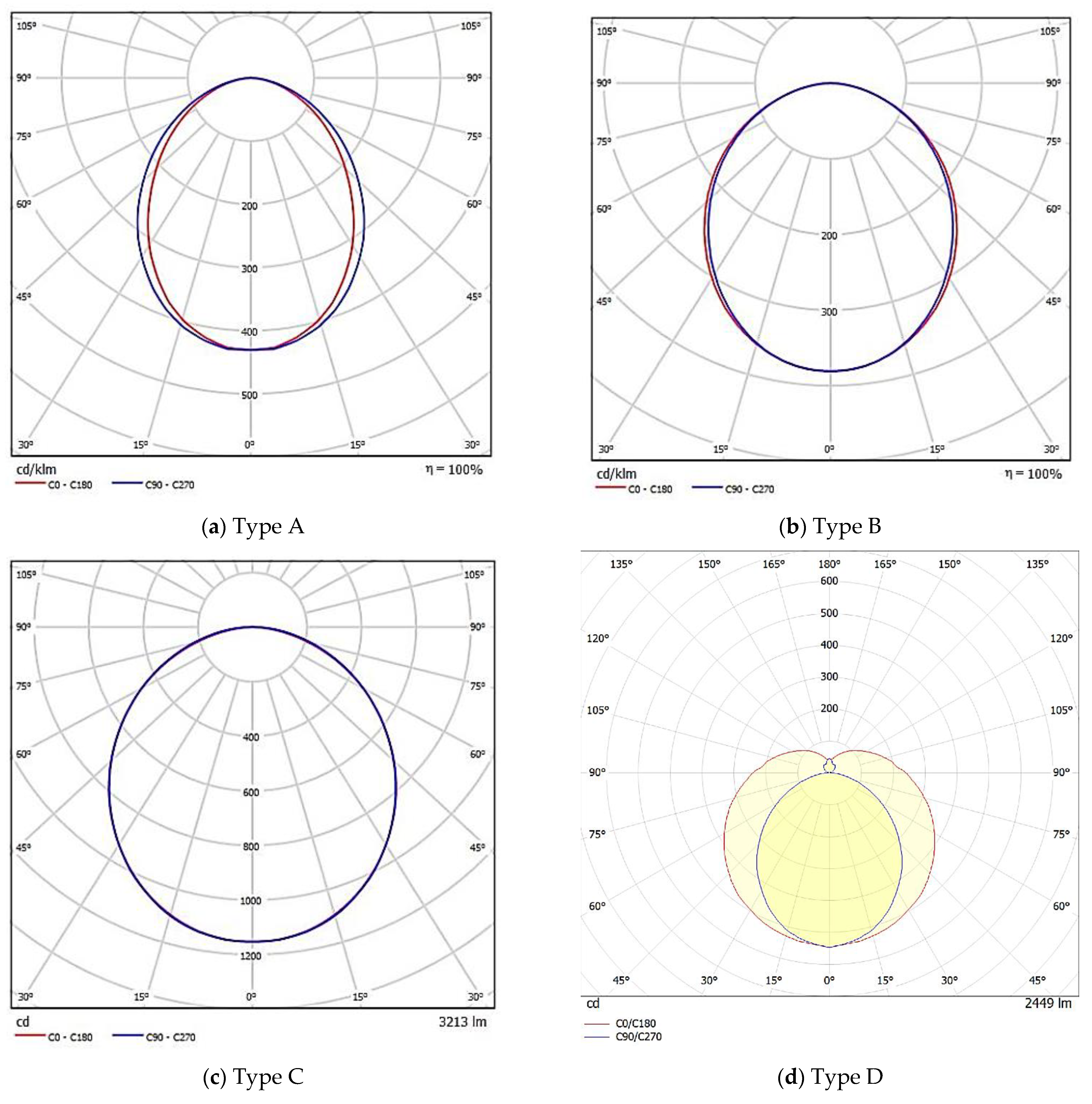
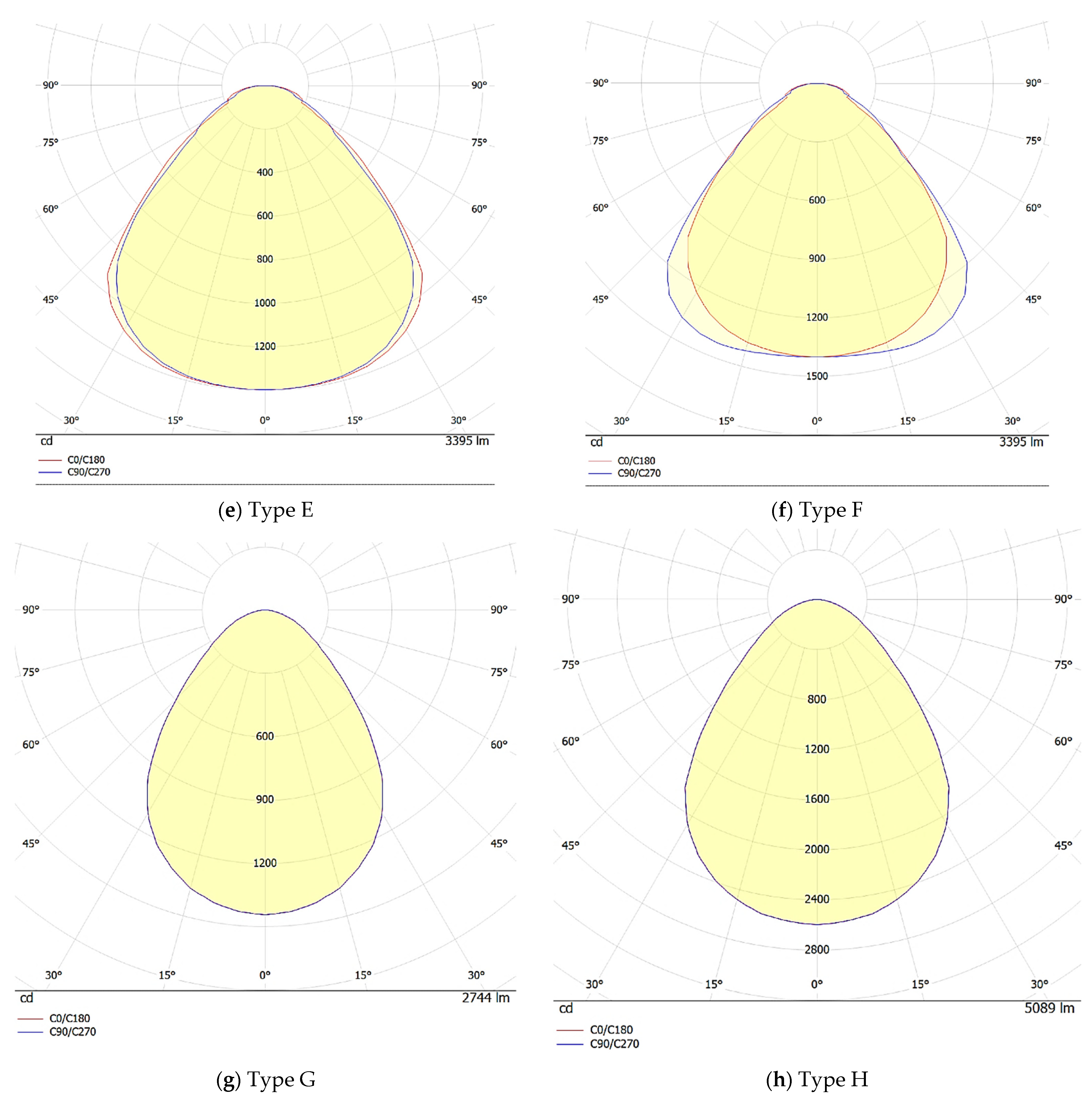
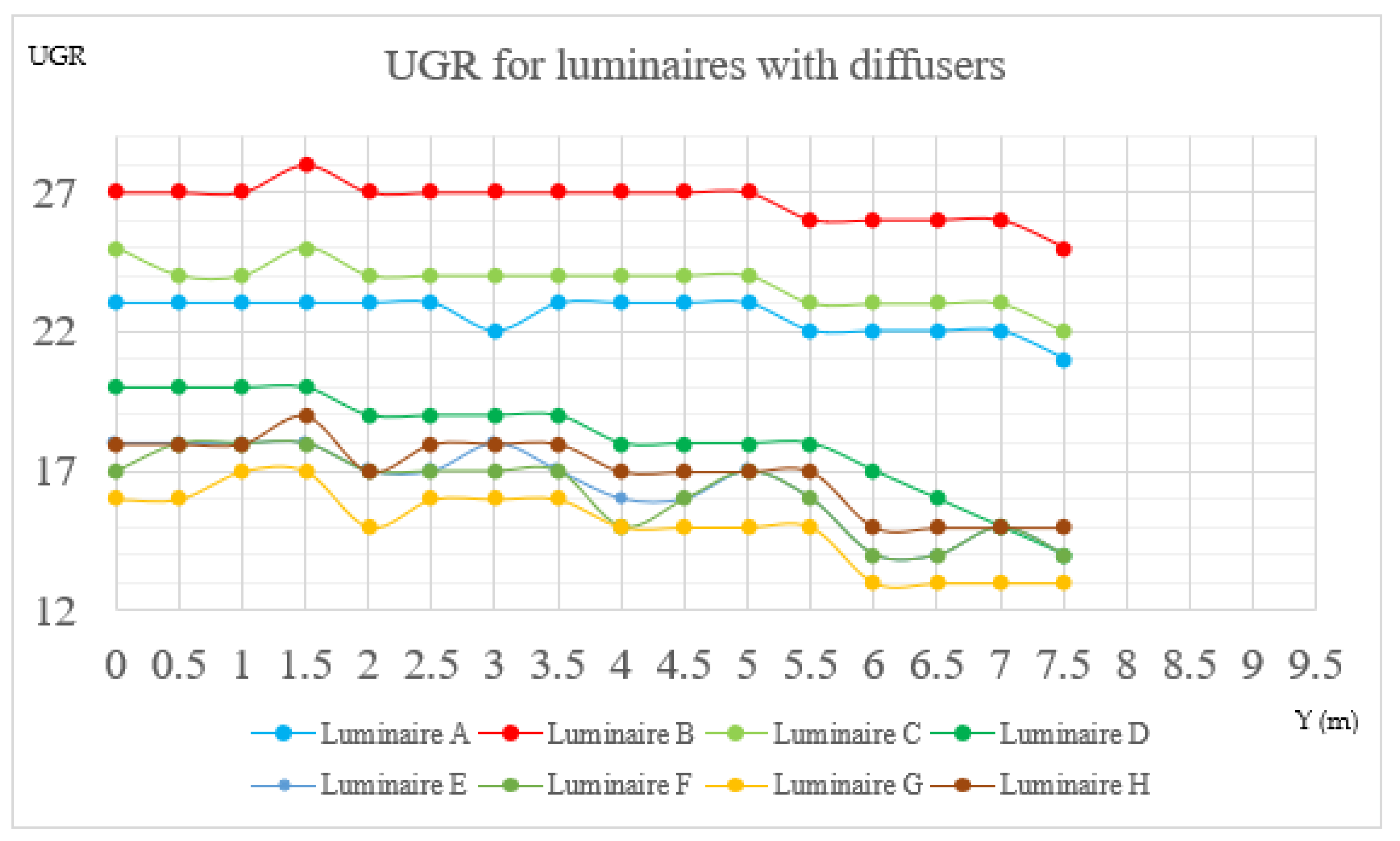
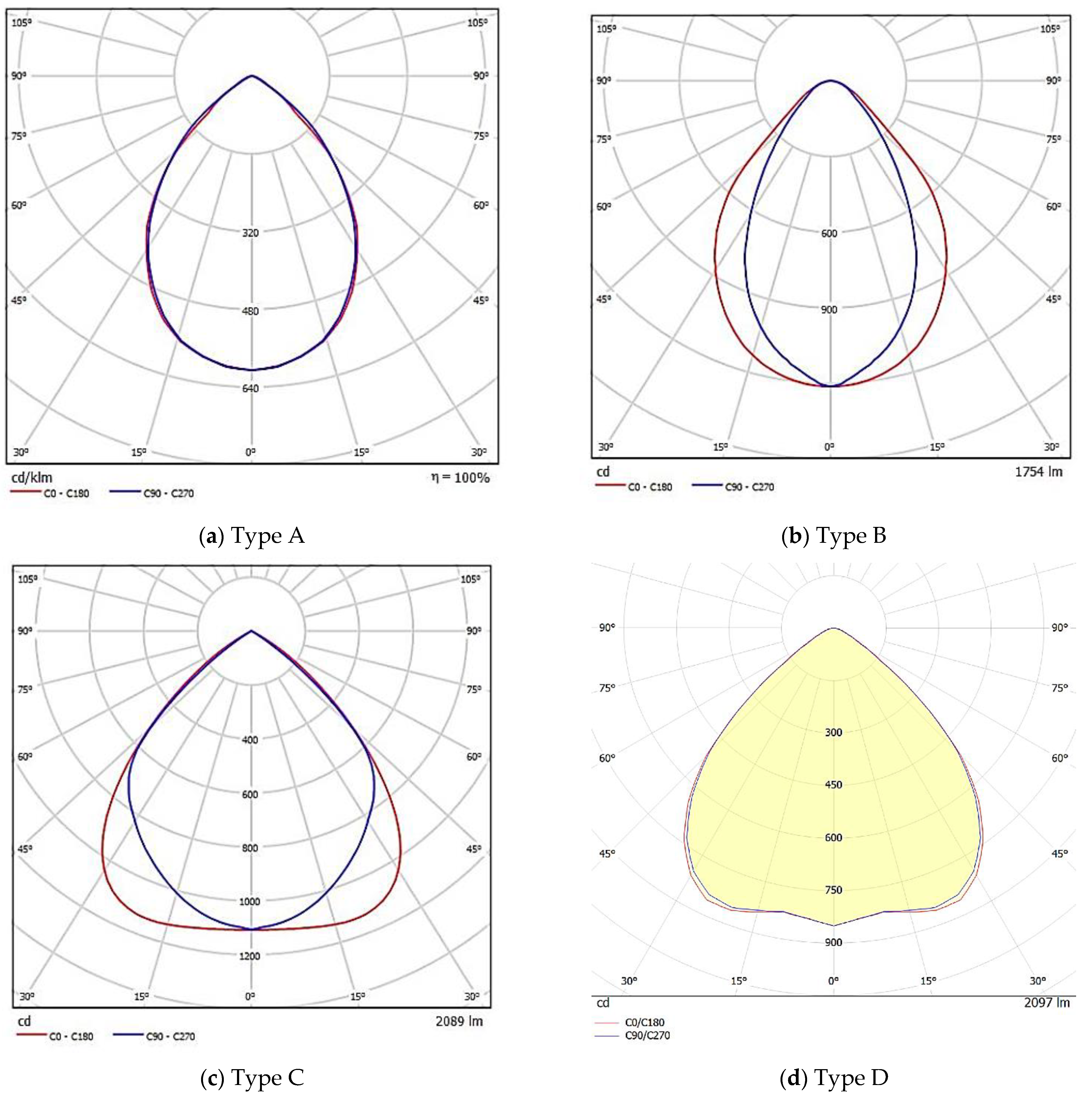
2.4.1. Luminaires Equipped with Diffusers (Uniform Luminous Intensity Distribution)

First, eight types of LED luminaire with diffusers are studied. The luminous intensity distribution for all the eight luminaire types can be seen in Figure 6a–h.

Although feasibility of the method is shown in Section 2.3 for luminaires with diffusers (uniform luminous intensity distribution), luminaires with variety in technical specification were selected for practical investigation of the method’s efficacy. The technical specifications of selected luminaires are illustrated in Table S5.

For studying eight types of LED luminaires with diffusers, UGR at the eye height of 1.2 m is simulated in DIALux software. The room size is $5\mathrm{H}\times 5\mathrm{H}$ and the observer moves on the room’s midline from the left wall to the right wall parallel to the luminaires’ axis. For meticulous calculation, UGR is simulated each 0.5 m of the observer’s path. Detailed results for all the types of luminaire are integrated and illustrated in Figure 7.

As can be seen in Figure 7, UGR changes for all LED luminaires with diffusers along the midline of the room were more or less similar. They started with a value which decreased after passing each row of the luminaires perpendicular to the observer’s viewing direction (moving path). After reaching the last two meters, the decrement became such that the UGR was under 10 units of UGR and was not given by the simulation software.

Due to the prevalence of LED luminaires with diffusers, it is helpful to find methods to calculate UGR for this type of luminaire in a reliable manner, with the smallest possible number of calculations, and with acceptable accuracy. In this research, a tabular approach is proposed for the estimation of the UGR of LED luminaires with diffusers, as well as conventional luminaire types with uniform luminous intensity distribution for UGR calculation reduction with acceptable accuracy.

For luminaires, manufacturers usually publish UGR calculating tables for obtaining UGR in the worst case, which corresponds to the midpoints of the walls. An example of a UGR table (luminaire with diffuser type A’s UGR table) is illustrated in Supplementary Table S1.

By accurate investigation of the curves in Figure 7 along with UGR tables published by manufacturers of eight types of LED luminaires with diffusers, a relation between them can be understood.

As explained before, the proposed method uses each number in the UGR table related to a room with dimensions corresponding to the observer’s position on a room midline. The X dimensions for two rooms are equal, but the Y dimension of the second (corresponding smaller) room is equal to the observer’s distance from the opposite-side wall in the observer’s field of view in the main room.

As showed mathematically in Section 2.3, the method works properly. For further validation of the method, examples for luminaires with luminous intensity distributions as in Figure 6a–h will be examined. By examining eight luminaires A to H and using two sets of the table data for X = 2H and 4H as well as Y = 2H, 3H, 4H, and 6H (as within the red border in Supplementary Table S1 and illustrated in Supplementary Tables S6–S13) for 2D interpolation or extrapolation, the similarities between the results of simulation and the proposed method for the mentioned types of luminaires are checked and confirmed (Tables S14–S21). X dimensions (2H and 4H) are selected since the room dimension 5H is near these two values and the ranges of Y from 2H, 3H, 4H, and 6H correspond to 4m, 6m, 8m, and 12 m, respectively, which properly cover the observer’s distance from 10 to 0 m from the opposite-side wall.

In Tables S14–S21, data obtained from simulation and 2D interpolation or extrapolation of UGR table data for $\mathrm{X}=10 m$ and $\mathrm{Y}=\left\{y| y=n\times {0.5}^m , n\in \mathbb{Z} \& 0\le n\le 19 \right\}$ for each type of luminaire with a diffuser are illustrated. Data used in the UGR table are for X = (2, 4) H and Y = (2, 3, 4, 6) H. The deviation of 2D-interpolated or extrapolated data average from the simulated UGR average for luminaires A to H is illustrated in

Table 5. The deviation of 2D-interpolated or extrapolated UGR average from the simulated UGR average for luminaires A to H.

Luminaire Type	A	B	C	D	E	F	G	H
Deviation of 2D-interpolated or extrapolated data from average of the simulated UGR as a percentage of 30 units of UGR.	−4.47%	−4.73%	−4.13%	−3.05%	1.71%	1.84%	0.07%	0.28%

as a percentage of 30 units of UGR. The maximum of absolute deviation is approximately 4.73% of 30 units of UGR. A perceptible change in UGR according to the Hopkinson criteria is 3 units, equaling 10% of 30 [19]. Therefore, deviation in the results of the proposed method is in the acceptable range. Additionally, from Supplementary Figures S1–S8, it is obvious that UGR obtained by 2D-interpolated or extrapolated table data follows the simulated UGR very closely. Therefore, for reducing UGR calculations in the indoor space, table data can be used. Hence, UGR at the calculation points, other than the wall midpoints, can be obtained from UGR tables.

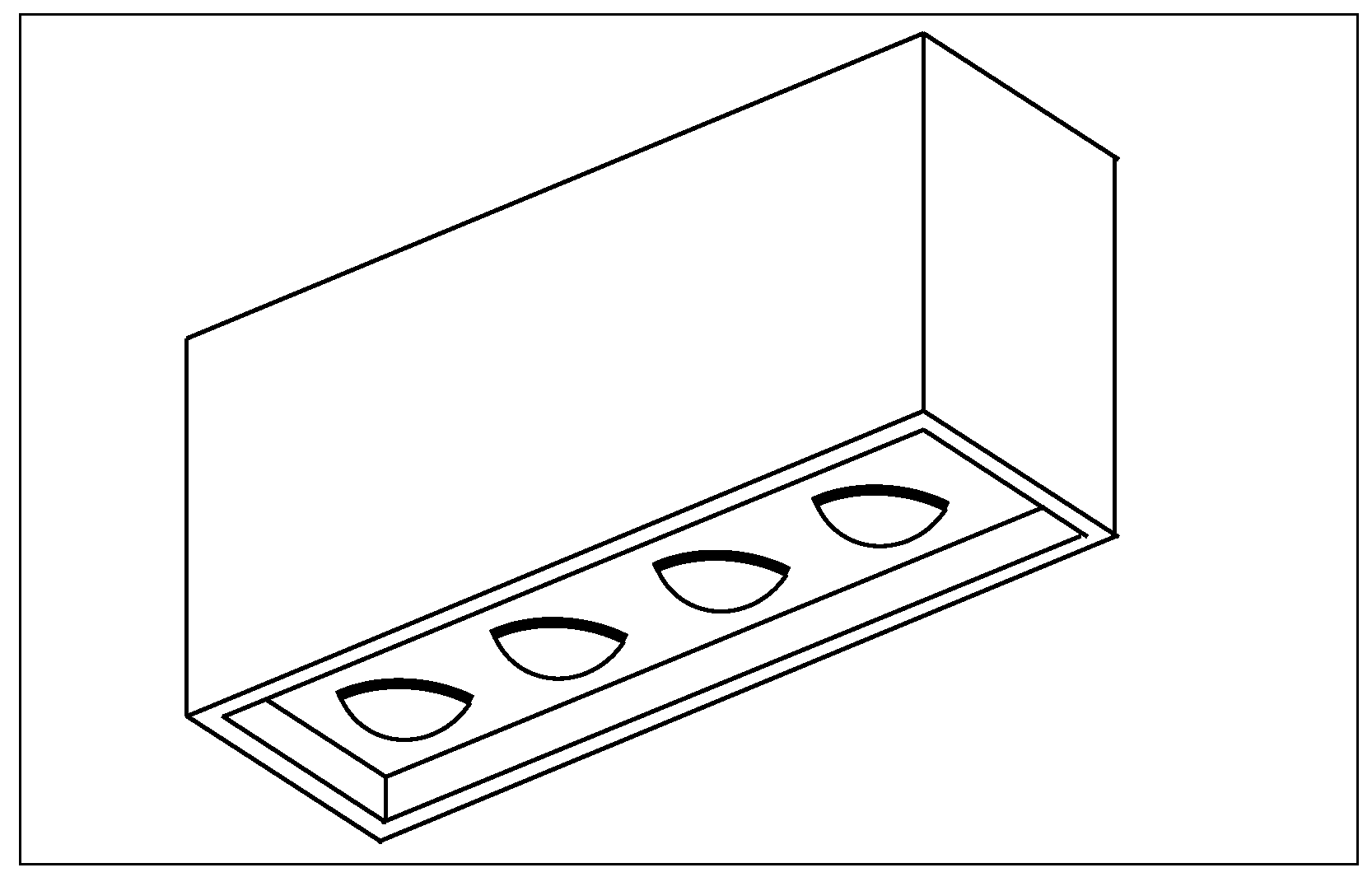
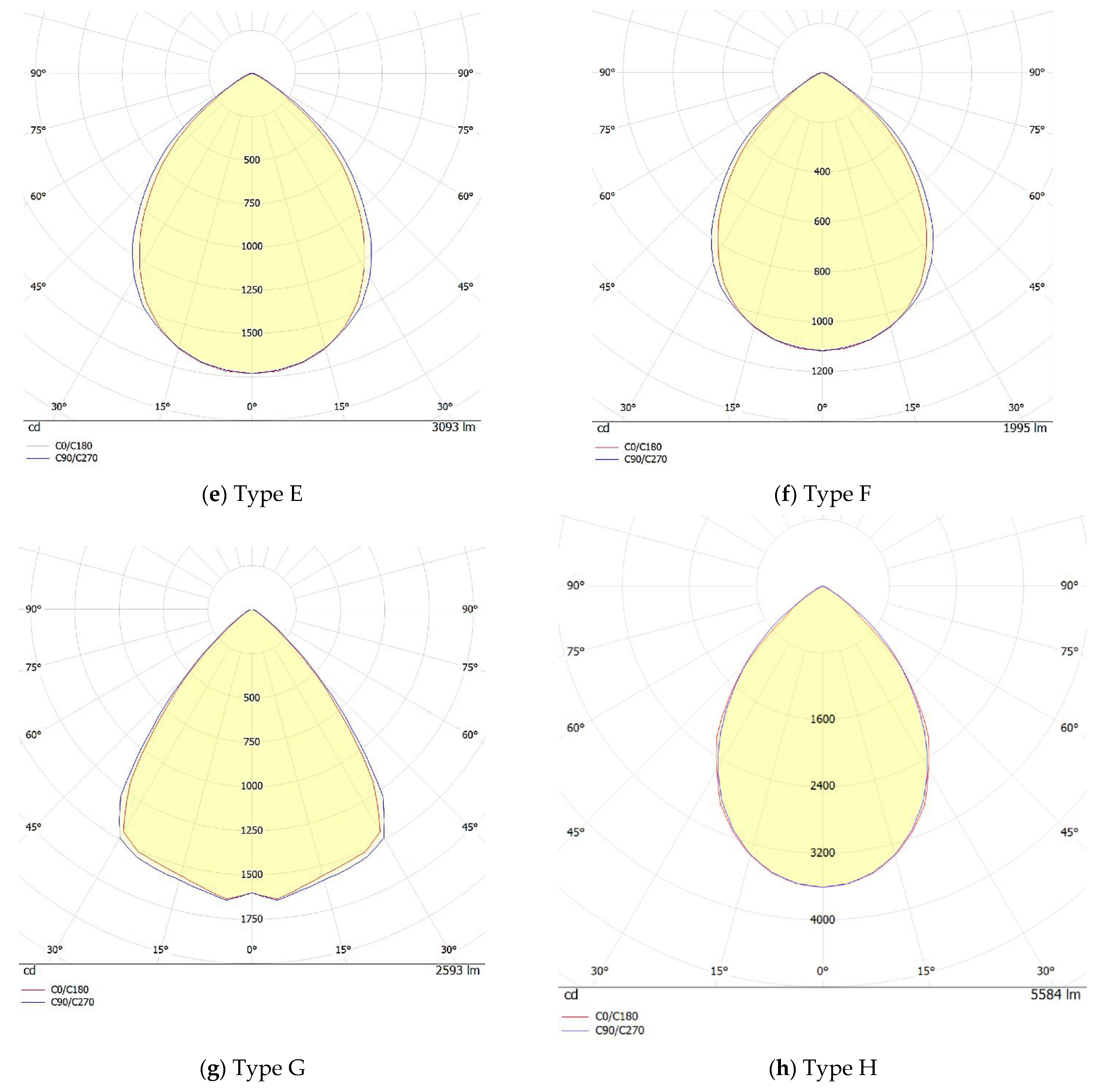
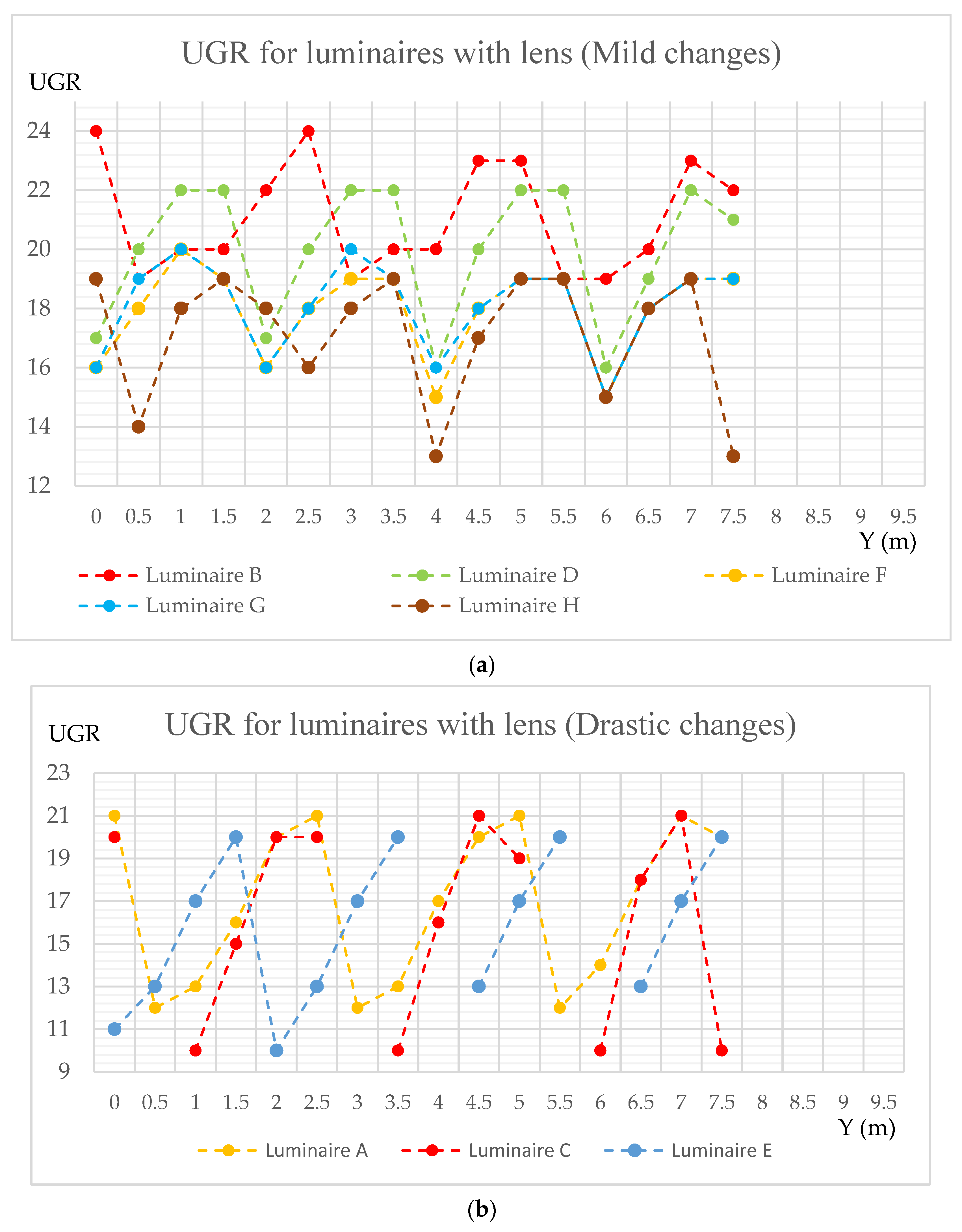
2.4.2. Luminaires Equipped with Lenses

Since in most applications, LED luminous flux must be formed to meet lighting needs, using lenses is one of the approaches for this aim [32]. Therefore, lenses as optical accessories enhance luminous intensity in LED luminaires in the required direction. An LED luminaire with lenses is illustrated in Figure 8.

Due to the popularity of LED luminaires with lenses, the UGR tabular calculation method proposed in this paper, with demonstrated validity for luminaires with diffusers (uniform luminous intensity distribution) and limitations explained in Section 2.3, is investigated in this case study to estimate efficacy of the method for luminaires with lenses.

Although the feasibility of the method was shown in Section 2.3 for luminaires with diffusers (uniform luminous intensity distribution), luminaires equipped with lenses with variety in technical specifications were selected for this case study. The technical specifications of selected luminaires are illustrated in Table S22.

For studying eight types of LED luminaires with lenses (luminous intensity distributions of the luminaires are illustrated in Figure 9a–h), UGR at an eye height of 1.2 m from the floor was simulated in DIALux software. The room size is $5\mathrm{H}\times 5\mathrm{H}$. The observer moves on the room’s midline from the left wall to the right wall of the room. For meticulous calculation, UGR is simulated in 0.5 m intervals and the results for all the types of luminaire are divided into luminaires with mild changes and those with drastic changes of UGR during the observer’s movement on the room’s midline, as illustrated in Figure 10a,b. Mild UGR changes correspond to UGR changes in a range of less than or equal to 6 units when the observer moves along the room’s midline. For drastic UGR changes, the range of change is more than 6 units.

As can be seen in Figure 10a,b, the change in UGR values for all LED luminaires with lenses along the midline of the room is more or less similar. They have an alternating behavior with a similar period. Luminaires E and C alternate drastically, while B, G, and F have smoother changes. For each luminaire type, the magnitude and the changes of the values are more or less similar along the observer’s path for each UGR curve.

The points which can be deduced from Figure 10a,b can be summarized as follows:

• Continuous curve represents lower contrast as UGR is a ratio of luminance (A, B, D, F, G and H).
• The average UGR matters (UGR of G < UGR of B).
• Discontinuous curve introduces a “torch” effect to the design (C and E).
• If UGR is not available, there is a chance that its value reaches 30 (E).

Due to the prevalence of LED luminaires with lenses, it is helpful if methods can be found to calculate UGR for this luminaire type in a reliable manner, with the lowest possible number of calculations, and with acceptable accuracy. As for LED luminaires with diffusers, the tabular method proposed in this research is also investigated for UGR estimation for LED luminaires with lenses. However, previously in Section 2.3, it was anticipated that the proposed method likely does not have enough efficacy for luminaires with non-uniform luminous intensity distribution.

An example of a UGR table (luminaire with lens type A’s UGR table) is illustrated in Table S23.

Similar to studying luminaires with diffusers, by accurately investigating the curves in Figure 10a,b along with UGR tables published by the manufacturers for eight types of LED luminaires with lenses, a relation between them can be understood. By examining eight luminaires A to H and using two sets of the table data for X = 2H and 4H and Y = 2H, 3H, 4H, and 6H (in the red border in Table S23, for example, and illustrated in Tables S24–S31) for 2D interpolation or extrapolation, the similarities between the proposed method and simulation results for the mentioned luminaires are checked (Tables S32–S39). X dimensions (2H and 4H) are selected since the room’s X dimension 5H is near these two values and the range of Y from 2H, 3H, 4H, and 6H corresponds to 4 m, 6 m, 8 m, and 12 m, respectively, which properly covers an observer’s distance from 10 to 0 m from the opposite-side wall in the room.

Tables S32–S39 show data obtained from 2D interpolation or extrapolation of table data and simulation data for $\mathrm{X}=10 m$ and $\mathrm{Y}=\left\{y| y=n\times {0.5}^m , n\in \mathbb{Z} \& 0\le n\le 19 \right\}$ for each luminaire with lenses. Data used in the UGR table is for X = (2, 4) H and Y= (2, 3, 4, 6) H. The deviation of 2D-interpolated or extrapolated data average from the simulated UGR average, for luminaires A to H, is illustrated in

Table 6. The deviation of 2D-interpolated or extrapolated data average from average of the simulated UGR as a percentage of 30 units of UGR for luminaires A to H.

Luminaire Type	A	B	C	D	E	F	G	H
Deviation of 2D-interpolated data average from average of the simulated UGR as a percentage of 30 units of UGR.	−3.59%	−23.4%	−12.83%	6.86%	5.40%	3.35%	3.10%	3.52%

as a percentage of 30 units of UGR. As mentioned before, according to Hopkinson criteria, below 10% deviation of full-scale UGR changing (0 to 30) is acceptable. Therefore, the proposed method results are not in the reliable range. Also, from Figures S9–S16, it is obvious that UGR obtained by 2D-interpolated or extrapolated table data does not properly follow the simulated UGR. In addition, for further study and finding any possibility for adapting the proposed tabular method for LED luminaires with lens (with non-uniform luminous intensity distribution), difference between UGR obtained by tabular method and simulation, according to supplementary Tables S32–S39 are illustrated in

Table 7. The deviation of 2D-interpolated or extrapolated UGR table data from the simulated UGR as a percentage of 30 units of UGR for luminaires A to H.

	Difference between Proposed Method and Simulation Results as a Percentage of 30 Units of UGR
Luminaire Type Observer Distance from Movement Starting Point (m)	A	B	C	D	E	F	G	H
2	13.33%	36.5%	12.17%	17.00%	24.33%	10.27%	10.67%	0.60%
4	3.33%	23.33%	7.67%	20.33%	- *	13.67%	10.67%	17.43%
6	5.50%	2.50%	10.33%	20.27%	- *	13.00%	13.33%	10.77%

* Difference is incalculable since simulation software according to UGR exceeding of 30 units limit does not calculate the UGR.

for distances from opposite-side wall equal to 4, 6, and 8 m separately. For mentioned distances from opposite-side wall, corresponding UGRs exist in UGR table and no interpolation or extrapolation in y axis is needed. From Table 7, it can be deduced that even at points that the UGR table directly gives UGR, there are great differences (more than 10% Hopkinson criterion as perceivable UGR change) between the proposed method and simulation results. Consequently, since the proposed tabular method is based on a UGR standard table which is constructed according to the standard UGR calculation method [4], and the result of the proposed method even for points the UGR table directly gives, the UGR value has great difference with results from simulation based on the standard UGR calculation formula. Hence, the UGR calculation method applicability for LED luminaires with lenses could be a unclear as stated in former research (e.g., [4,7]). Therefore, further research and efforts to enhance the usual method are needed to find ways for accurate UGR calculation for luminaires with non-uniform luminous intensity distribution, including LED luminaires equipped with lenses. Consequently, as a UGR-calculation-reducing method in indoor spaces along room midlines for luminaires with lenses, the table data cannot be used. This corresponds exactly to what was anticipated for proposed method efficacy for LED luminaires with lenses in Section 2.3.

3. Conclusions

In this paper, a comprehensive investigation was performed on the efficacy of the proposed easy-to-use and calculation-reducing method for UGR calculation for LED luminaires. UGR as a metric for evaluation of indoor lighting user visual discomfort is introduced in related standards, and advised UGR values should be observed by indoor lighting designers. Indoor lighting designers must simulate their designation to find out whether it meets the standard limits or not. The proposed method makes it possible to find by referral to the UGR table given by the manufacturer, or by an interpolation or extrapolation of the table numbers, the UGR of points on the room’s midline. Efficacy and validation limits of the proposed method were mathematically proved and discussed in detail. Since LED luminaires have attracted great attention, it is crucial that approaches be found to calculate UGR while consuming less time and energy. For luminaires with diffusers or uniform luminous intensity distribution, the tabular method was proved, calculated, and simulated. The results confirmed the validity of this method.

For luminaires with lenses, as in the method proof anticipated, the tabular method failed to model the UGR accurately. It can be based on non-uniform luminous intensity distribution of these types of luminaires. Further research is needed for modelling and finding a fast and easy-to-use way to calculate UGR for LED luminaires with lenses.

References

1. Carlucci, S.; Causone, F.; De Rosa, F.; Pagliano, L. A review of indices for assessing visual comfort with a view to their use in optimization processes to support building integrated design. Renew. Sustain. Energy Rev. 2015, 47, 1016–1033. [Google Scholar] [CrossRef] [Green Version]
2. González-Torres, M.; Pérez-Lombard, L.; Coronel, J.F.; Maestre, I.R.; Yan, D. A review on buildings energy information: Trends, end-uses, fuels and drivers. Energy Rep. 2021, 8, 626–637. [Google Scholar] [CrossRef]
3. Moadab, N.H.; Olsson, T.; Fischl, G.; Aries, M. Smart versus conventional lighting in apartments—Electric lighting energy consumption simulation for three different households. Energy Build. 2021, 244, 111009. [Google Scholar] [CrossRef]
4. Erdem, L.; Trampert, K.; Neumann, C. Evaluation of discomfort glare from LED lighting systems. Ing. Iluminatului 2012, 14, 2. [Google Scholar]
5. Fontoynont, M. LED lighting, ultra-low-power lighting schemes for new lighting applications. Comptes Rendus. Phys. 2018, 19, 159–168. [Google Scholar] [CrossRef]
6. Wolska, A.; Sawicki, D. Practical application of HDRI for discomfort glare assessment at indoor workplaces. Measurement 2020, 151, 107179. [Google Scholar] [CrossRef]
7. Iacomussi, P.; Radis, M.; Rossi, G.; Rossi, L. Visual Comfort with LED Lighting. Energy Procedia 2015, 78, 729–734. [Google Scholar] [CrossRef] [Green Version]
8. CIE 117; Discomfort Glare in Interior Lighting, Technical Report; International Comission on Illumination: Vienna, Austria, 1995; ISBN 9783900734701.
9. Slominski, S. Potential Resource of Mistakes Existing While Using the Modern Methods of Measurement and Calculation in the Glare Evaluation. In Proceedings of the 2016 IEEE Lighting Conference of the Visegrad Countries, Lumen V4, Karpacz, Poland, 13–16 September 2016; pp. 1–5. [Google Scholar] [CrossRef]
10. Tsankov, P.; Yovchev, M. Measurement and Determination of the Unified Glare Rating of Indoor Lighting Systems. In Proceedings of the 2018 Seventh Balkan Conference on Lighting (BalkanLight), Varna, Bulgaria, 20–22 September 2018; pp. 1–6. [Google Scholar] [CrossRef]
11. Scheir, G.; Hanselaer, P.; Ryckaert, W. Pupillary light reflex, receptive field mechanism and correction for retinal position for the assessment of visual discomfort. Light. Res. Technol. 2017, 51, 291–303. [Google Scholar] [CrossRef]
12. Quek, G.; Wienold, J.; Khanie, M.S.; Erell, E.; Kaftan, E.; Tzempelikos, A.; Konstantzos, I.; Christoffersen, J.; Kuhn, T.; Andersen, M. Comparing performance of discomfort glare metrics in high and low adaptation levels. Build. Environ. 2021, 206, 108335. [Google Scholar] [CrossRef]
13. Fotios, S.; Kent, M. Measuring Discomfort from Glare: Recommendations for Good Practice. LEUKOS 2020, 17, 338–358. [Google Scholar] [CrossRef]
14. Kent, M.; Fotios, S.; Altomonte, S. Discomfort glare evaluation: The influence of anchor bias in luminance adjustments. Light. Res. Technol. 2017, 51, 131–146. [Google Scholar] [CrossRef]
15. Pierson, C.; Wienold, J.; Bodart, M. Review of Factors Influencing Discomfort Glare Perception from Daylight. LEUKOS 2018, 14, 111–148. [Google Scholar] [CrossRef]
16. Wienold, J.; Iwata, T.; Khanie, M.S.; Erell, E.; Kaftan, E.; Rodriguez, R.; Garreton, J.Y.; Tzempelikos, T.; Konstantzos, I.; Christoffersen, J.; et al. Cross-validation and robustness of daylight glare metrics. Light. Res. Technol. 2019, 51, 983–1013. [Google Scholar] [CrossRef] [Green Version]
17. Donners, M.A.H.; Vissenberg, M.; Geerdinck, L.M.; van den Broek-Cools, J.H.F.; Buddemeijer-Lock, A. A psychophysical model of discomfort glare in both outdoor and indoor applications. In Proceedings of the 28th CIE Session, Manchester, UK, 28 June–4 July 2015; Volume 216, p. 2015. [Google Scholar]
18. Porsch, T.; Funke, C.; Schmidt, F.; Schierz, C. Measurement of the Unified Glare Rating (UGR) Based on Using ILMD. In Proceedings of the 28th CIE Session, Manchester, UK, 28 June–4 July 2015. [Google Scholar]
19. Scheir, G.H.; Hanselaer, P.; Bracke, P.; Deconinck, G.; Ryckaert, W.R. Calculation of the Unified Glare Rating based on luminance maps for uniform and non-uniform light sources. Build. Environ. 2015, 84, 60–67. [Google Scholar] [CrossRef]
20. Scheir, G.H.; Hanselaer, P.; Ryckaert, W.R. Defining the Actual Luminous Surface in the Unified Glare Rating. LEUKOS 2017, 13, 201–210. [Google Scholar] [CrossRef]
21. Bangali, J. Discomfort glare prediction by using Unified Glare Rating. Aust. J. Electr. Electron. Eng. 2018, 15, 184–191. [Google Scholar] [CrossRef]
22. Tyukhova, Y.; Waters, C.E. Discomfort Glare from Small, High-Luminance Light Sources When Viewed against a Dark Surround. LEUKOS 2018, 14, 215–230. [Google Scholar] [CrossRef]
23. Sharma, D.; Bhardwaj, A.; Sharma, M.; Mirza, A. Qualitative and quantitative analysis of discomfort glare due to artificial indoor lighting. Int. J. Product. Qual. Manag. 2019, 28, 90–102. [Google Scholar] [CrossRef]
24. Chaudhry, A.U. (Ed.) Application of Fluid Flow Equations to Gas Systems; Gulf Professional Publishing: Burlington, UK, 2003; Chapter 2; pp. 11–83. [Google Scholar]
25. Maurin, A.; Kwapisz, L. Simplified method for calculating airborne sound transmission through composite barriers. Compos. Struct. 2021, 276, 114526. [Google Scholar] [CrossRef]
26. Chakrabarty, A.; Mannan, S.; Cagin, T. (Eds.) Inherently Safer Design; Butterworth-Heinemann: Boston, MA, USA, 2016; Chapter 8; pp. 339–396. [Google Scholar]
27. Jarungthammachote, S. Simplified model for estimations of combustion products, adiabatic flame temperature and properties of burned gas. Therm. Sci. Eng. Prog. 2020, 17, 100393. [Google Scholar] [CrossRef]
28. AS/NZS 1680 Interior Lighting. 2009. Available online: www.standards.co.nz (accessed on 21 February 2022).
29. Kong, Q.; Siauw, T.; Bayen, A.M. Python Programming and Numerical Methods: Interpolation; Academic Press: Cambridge, MA, USA, 2021; Chapter 17; pp. 295–313. [Google Scholar] [CrossRef]
30. Farin, G. Tensor Product Patches; Elsevier BV: Amsterdam, The Netherlands, 2002; pp. 245–268. [Google Scholar]
31. Calculation and Presentation of Unified Glare Rating Tables for Indoor Lighting Luminaires; CIE 190; CIE: Vienna, Austria, 2010.
32. Ding, Y.; Liu, X.; Zheng, Z.-R.; Gu, P.-F. Freeform LED lens for uniform illumination. Opt. Express 2008, 16, 12958–12966. [Google Scholar] [CrossRef] [PubMed] [Green Version]
Figure 1. Visual discomfort glare of luminaires installed in the ceiling in a closed space.
Applsci 12 03462 g001
Figure 2. Illustrating the points UGR table was originally designed for (black arrows), and points for which the UGR table can be used (red lines).
Applsci 12 03462 g002
Figure 3. Illustration of the part of the main room (in grey color) which is used as a new room with different dimensions for UGR calculation in the proposed method.
Applsci 12 03462 g003
Figure 4. (a) Observer in a position in a room in which some of the luminaires are in front of them (in their field of view), (b) observer in a room which contains only the luminaires that are in the first observer’s field of view.
Applsci 12 03462 g004
Figure 5. N A W as a function of X and Y (room dimensions).
Applsci 12 03462 g005
Figure 6. (ah) (Luminaires types A–H) Luminous intensity distribution of the eight types of luminaires with diffusers studied in this research.
Applsci 12 03462 g006aApplsci 12 03462 g006b
Figure 7. Eight LED luminaires’ UGR curves (luminaires described in Figure 6a–h) along the room’s midline when observer’s viewing direction is parallel to the luminaires’ axis.
Applsci 12 03462 g007
Figure 8. A sample LED luminaire with lenses.
Applsci 12 03462 g008
Figure 9. (ah). (Luminaires types A–H) Luminous intensity distribution of eight luminaires with lenses studied in this research.
Applsci 12 03462 g009aApplsci 12 03462 g009b
Figure 10. Eight LED luminaires’ UGR curves (a) for luminaires with UGR mild changes ( m a x m i n UGR 6), and (b) for drastic changes of UGR ( m a x m i n UGR > 6) along the room’s midline. (For luminaires described in Figure 9a–h along the room’s midline when the observer’s viewing direction is parallel to the luminaires’ axis).
Applsci 12 03462 g010