On the Design of Regulation Controllers for Automation Systems with RCPetri

Abstract

Regulation control for Petri nets is a control framework that allows the design of sequence controllers for automation systems in a systematic and efficient way. In order to implement this control framework, the MATLAB^® app RCPetri has been developed. In this work, the RCPetri tool functionalities are described, including model generation, automatic specification generation, automatic control design, model and control simulation, automatic translation to PLC code, and communication by Modbus TCP/IP and OPC UA. Furthermore, three examples are presented to illustrate the application of the tool and the regulation framework: an electro-pneumatic device, a process control system, and a robotic manufacturing cell under a decentralized control scheme.

1. Introduction

Petri nets ($PNs$) is a family of mathematical models that have been extensively used for representing and analyzing systems that evolve through the occurrence of events named discrete event systems [1,2,3]. Applications include the analysis of traffic [4], risk assessment [5], biological systems [6], logistics [7,8], and manufacturing systems [9], among others.

One application of $PNs$ that has received a lot of attention in the literature is the design of control algorithms for manufacturing systems. The most common approach consists of the design of places (monitors) that control the firing of transitions, in order to impose a requirement described as a linear inequality, named generalized mutual exclusion constraint (GMEC) [10,11,12,13]. These constraints are useful to enforce safety specifications, avoiding states when two or more processes use the same resource. This control technique has also been extensively investigated to avoid blocking states in particular classes of $PNs$ (see, for instance, [14,15,16,17]). A recent survey on the control of $PNs$ can be found in [18].

Regulation control [19,20,21] is a different control paradigm, the objective of which is to design controllers that impose sequences of sensors and actuators activation. In detail, the system to be controlled, named Plant, is modeled as an Interpreted Petri net ($IPN$), which is an extension of $PNs$ with labels associated with places (representing sensors) and transitions (representing actuators). The required behavior is described as an $IPN$ as well, named Specification, representing required sequences of sensors and actuators activation. Then, a controller is designed as an $IPN$ that enforces the Plant to evolve according to the given Specification. Common problems in automation systems, where the engineer requires to program a routine so the Plant describes a required operations sequence, can be addressed by this approach. The advantage of using this scheme is that the engineer only specifies the required tasks in a high-level description; next, the controller can be automatically generated by using the algorithms that have been developed for this purpose [19,20,21]. Furthermore, once the $IPN$ controller is designed, it can be automatically translated into programmable logic controller (PLC) code for implementation.

In order to perform a practical implementation of the regulation control approach, we have developed a MATLAB^® app named RCPetri [22], which is described in this work. The app was designed to help the user to design and implement regulation controllers by following a control design workflow. In a first step, the app allows us to define an $IPN$ that represents the Plant in a graphical way. Next, the user can define the required behavior in high-level fashion by using standard Excel tables, which are automatically translated by the app to an $IPN$ Specification. Later, the controller can be automatically generated. Furthermore, the closed-loop system can be simulated to verify the behavior of the Plant under control. Moreover, the $IPN$ controller can be automatically translated into PLC code, for its final implementation. Furthermore, a communication module has been implemented, which allows synchronization with other software or hardware through protocols Modbus Internet Protocol Suite (Modbus TCP/IP) and object linking and embedding for process-control-unified architecture (OPC UA). In order to illustrate the use of the app for the synthesis of controllers and their application, three examples are described, as follows:

1.

An electro-pneumatic arm that can perform four different tasks, whose controller is implemented in a PLC;

2.

A process control system simulated in a supervisory control and data acquisition (SCADA) software synchronized to the app via Modbus TCP/IP;

3.

A manufacturing system with two robotic cells, simulated in a dedicated software and synchronized to the app via an OPC UA server, under a decentralized control scheme.

Different research groups have developed software tools for modeling and analyzing different $PN$ types. For instance, GreatSPN [23] and PIPE2 [24] are well-known tools for performance analysis in generalized stochastic $PNs$. TimeNET [25] allows the analysis of non-Markovian stochastic $PNs$. Similarly, GPenSIM [26] can be used for performance evaluation in event graphs. CPN Tools [27] and Access/CPN [28] were proposed for the modeling, simulation, and analysis of colored $PNs$. Continuous and hybrid $PNs$ can be simulated in HYPENS [29] and SimHPN [30]. PNetLab [31] was developed to model and simulate timed/untimed $PNs$ and colored $PNs$, allowing the possibility to simulate $PNs$ under control, where the controller is a subroutine that provides a conflict resolution policy. In [32], a combination of the graphical editor Petri Net Editor and the toolbox Petri Net Engine is used to implement a $PN$ conflict resolution policy into a microcontroller. All of these tools allow us to graphically define a $PN$ system, simulate the system, and perform particular types of analysis (mainly performance analysis and structural analysis). Nevertheless, despite the large amount of $PN$ software, none of the existing tools allow us to define $IPN$ with place and transition labels, and to synthesize regulation controllers. Moreover, to the best of our knowledge, none of the tools allow us to synchronize $PN$ simulations with external software/hardware via standard protocols, and to automatically generate PLC code. Furthermore, the implementation of RCPetri on MATLAB^® will allow other researchers to use it for the analysis and application of other algorithms, such as GMEC control, $PN$ observers, and $PN$ diagnosers, among others.

This paper is organized as follows: Section 2 presents basic definitions on $IPN$. Section 3 explains the regulation control framework. Section 4 introduces the RCPetri app with its main features, and the algorithms implemented for the main functionalities. Section 5 presents the application of RCPetri in the three examples previously mentioned. Section 6 summarizes the conclusions.

2. Basic Concepts

Basic concepts and definitions concerning $PNs$ and $IPN$ are recalled in this section (for more details see, for instance [3,33]).

Definition 1.

A Petri net ($PN$) structure, $\mathcal{N}$, is a bipartite digraph represented by the 4-tuple $\mathcal{N}=〈P,T,I,O〉$, where $P=\{p_1,p_2,...,p_n\}$ is the finite set of places, $T=\{t_1,t_2,...,t_m\}$ is the finite set of transitions, $I:P\times T\to {\mathbb{N}}_0$ is a function representing weighted arcs connecting places to transitions, and $O:P\times T\to {\mathbb{N}}_0$ is a function representing weighted arcs connecting transitions to places.

The incidence matrix of $\mathcal{N}$ is defined as a $\left|P\right|\times \left|T\right|$ matrix $\mathbf{C}$, such that $\mathbf{C}[i,j]=O(p_i,t_j)-I(p_i,t_j)$, $\forall p_i\in P,\forall t_j\in T$. Graphically, places are represented by circles, transitions by rectangles, and arcs by arrows. Given a node $v\in P\cup T$, ${}^{•}v$ (resp. $v^{•}$) denotes the set of nodes directly connected to v (resp. nodes directly connected from v). A $PN$ is said to be a state machine if each transition has only one input and one output place (i.e., $\forall t\in T$${|}^{•}t|=|t^{•}|=1$) and the Petri net graph is strongly connected.

Definition 2.

An Interpreted Petri net ($IPN$) system is a 8-tuple $Q=〈\mathcal{N},M_0,{\Sigma }_I$, ${\Sigma }_{Id},{\Sigma }_O,{\lambda }_I$, ${\lambda }_{Id},\phi 〉$, where:

• $\mathcal{N}$ is a $PN$;
• $M_0$ is the initial marking, defined as a function, $M_0:P\to {\mathbb{N}}_0$, describing the number of tokens (dots) initially residing inside each place;
• ${\Sigma }_I$ is the input alphabet—each element of ${\Sigma }_I$ is an input symbol;
• ${\Sigma }_{Id}$ is the identity alphabet—each element of ${\Sigma }_{Id}$ is an identity symbol;
• ${\Sigma }_O$ is the output alphabet—each element of ${\Sigma }_O$ is an output symbol;
• ${\lambda }_I:T\to 2^{{\Sigma }_I}$ is the input labeling function that associates transitions to input symbols. A transition can be associated with several input symbols. If ${\lambda }_I\left(t_j\right)\ne \varnothing$, then the transition $t_j$ is said to be controllable, otherwise it is uncontrollable;
• ${\lambda }_{Id}:T\to {\Sigma }_{Id}\cup \left\{ϵ\right\}$ is the identity labeling function, where two transitions cannot have the same identity label and each transition can have one identity label at most; ϵ represents that the transition has not identity label;
• $\phi :P\to 2^{{\Sigma }_O}$ is the output labeling function that associates places to output symbols. A place can be associated with several output symbols.

The marking distribution of an $IPN$ describes the state of the represented dynamical system; the marking changes according to the following rules:

• Given a current marking distribution, $M_k:P\to {\mathbb{N}}_0$, an external observer reads the symbols associated with the marked places, whose set is denoted as $\phi \left(M_k\right)=\{o\in {\Sigma }_O|o\in \phi \left(p\right),M_k\left(p\right)>0\}$. $\phi \left(M_k\right)$ is said to be the current output of the $IPN$ and the symbols of $\phi \left(M_k\right)$ are said to be indicated at $M_k$.
• A transition $t_j$ is said to be marking-enabled at marking $M_k$ if $\forall p_i\in {}^{•}{t}_j$, $M_k\left(p_i\right)\ge I(p_i,t_j)$.
• A transition $t_j$ is said to be label-enabled at marking $M_k$ if every symbol $a\in {\lambda }_I\left(t_j\right)$ is indicated by either the current marking $M_k$ or an external agent. If $\lambda \left(t_j\right)=\varnothing$, then $t_j$ is always label-enabled.
• If $t_j$ is marking-enabled and label-enabled at $M_k$, then it is said to be enabled, and it can be fired (denoted as $M_k[t_j>$). Otherwise, it is said to be disabled.
• The firing of a transition $t_j$, enabled at $M_k$, leads to a new marking $M_{k+1}$ (denoted as $M_k[t_j>M_{k+1}$), caused by removing $I(p_i,t_j)$ tokens to each place $p_i\in {}^{•}{t}_j$ and adding $O(p_i,t_j)$ tokens to each place $p_i\in {t_j}^{•}$.

The marking function M can be expressed as a column vector $\mathbf{M}\in {\mathbb{N}}_0^{\left|P\right|}$, such that $\mathbf{M}\left[i\right]=M\left(p_i\right)$, $\forall p_i\in P$. In this work, both M and $\mathbf{M}$ will be called marking, since both represent the same information. Thus, a marking $M_{k+1}$, reached from $M_k$ after firing a transition $t_j$, can be computed as ${\mathbf{M}}_{k+1}={\mathbf{M}}_k+\mathbf{C}\overrightarrow{t_j}$, where $\overrightarrow{t_j}$ is the j-th column of the identity matrix of dimension $\left|T\right|$. The function $\phi$ can be represented by a $|{\Sigma }_O|\times |P|$ matrix $\phi$, in which $\phi [i,j]=1$, if $p_j$ is labeled with the i-th output symbol and $\phi [i,j]=0$ otherwise. The output vector of the $IPN$ at $M_k$ is defined as ${\mathbf{y}}_k=\phi {\mathbf{M}}_k$.

A firing sequence is a sequence of transitions $\sigma =t_i{t}_j\cdots t_k$, such that $M_0[t_i>M_1[t_j>\cdots M_m[t_k>M_{m+1}$. The marking ${\mathbf{M}}^{\prime }$ reached after the firing of $\sigma$ from a marking $\mathbf{M}$ can be computed as ${\mathbf{M}}^{\prime }=\mathbf{M}+\mathbf{C}\overrightarrow{\sigma }$, where $\overrightarrow{\sigma }\in {\mathbb{N}}_0^{\left|T\right|}$ is a column vector, named the Parikh vector, defined such that $\overrightarrow{\sigma }\left[j\right]=k$, if $t_j$ is fired k times in $\sigma$. This is denoted as $M[\sigma >M^{\prime }$, and  $M^{\prime }$ is said to be reachable from M.

A $PN$ system is said to be bounded if $\exists k\in \mathbb{N}$, such that $\forall p\in P$ and for any M reachable from $M_0$, it holds that $M\left(p\right)\le k$. A $PN$ system is said to be safe if it is bounded with $k=1$. A $PN$ system is said to be live if $\forall t_j\in T$ and for any M reachable from $M_0$ there exists a fireable sequence $\sigma$, such that $M[\sigma >M^{\prime }$ and $t_j$ is (marking) enabled at $M^{\prime }$.

$IPN$ models for complex systems can be built from $IPN$ component models, by using the synchronous composition. Given two safe $IPN$$Q^1$ and $Q^2$, the synchronous composition results in another safe $IPN$$Q^3=Q^1\parallel Q^2$, defined as the union of $Q^1$ and $Q^2$ in which the transitions sharing the same identity label are merged, keeping all the transition and place labels. The synchronous composition is commutative and associative.

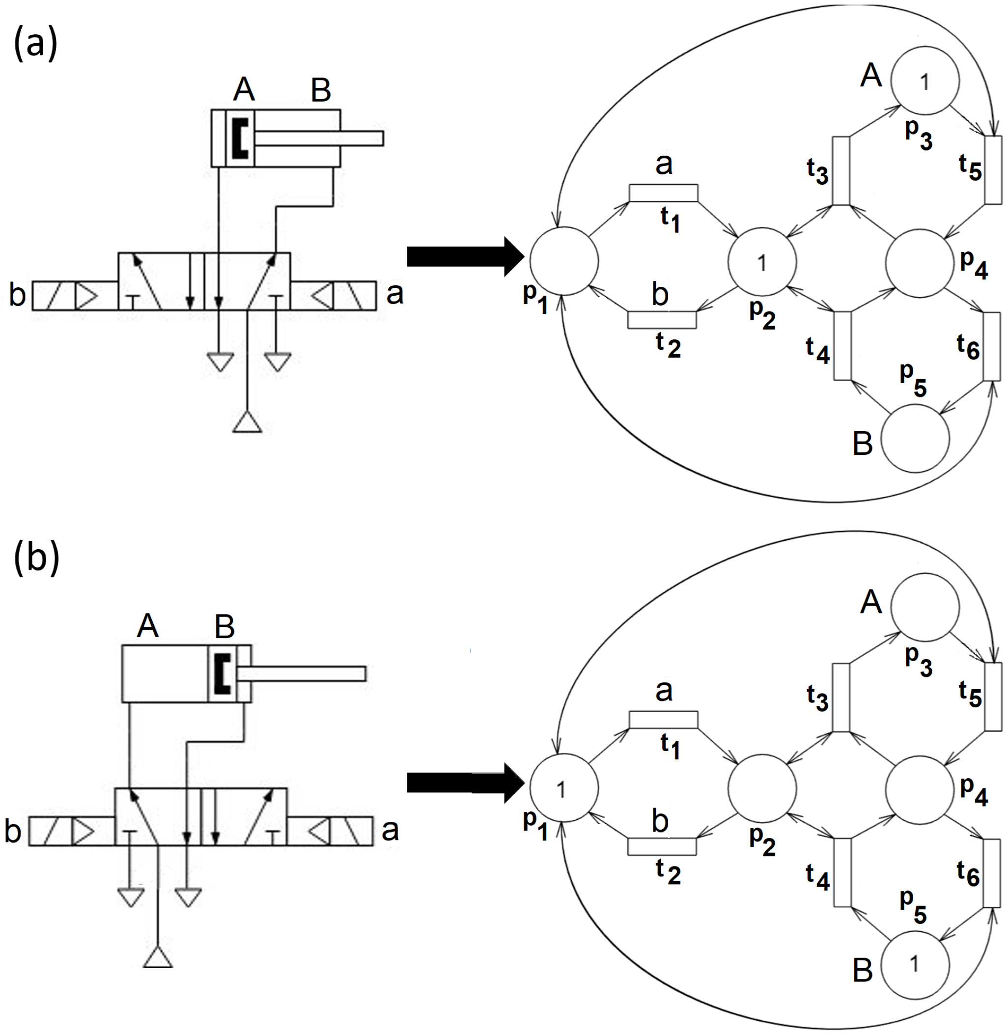
Example 1.

Consider the double-acting electro-pneumatic actuator driven by a 5/2 valve and its $IPN$ model shown in Figure 1. The incidence matrixCand the output labeling matrix φ is given by the following:

$$\mathit{C}=\left[\begin{array}{cccccc}-1& 1& 0& 0& 0& 0\\ 1& -1& 0& 0& 0& 0\\ 0& 0& 1& 0& -1& 0\\ 0& 0& -1& 1& 1& -1\\ 0& 0& 0& -1& 0& 1\end{array}\right],\mathit{\phi }=\left[\begin{array}{ccccc}0& 0& 1& 0& 0\\ 0& 0& 0& 0& 1\end{array}\right].$$

The input alphabet is defined as ${\Sigma }_I=\{a,b\}$, where each symbol represents a command signal that allows the change of the valve position (i.e., energizing a coil), which leads to an actuator movement. The output alphabet is defined as ${\Sigma }_O=\{A,B\}$, where each symbol represents the activation of a sensor witnessing the actuator position. Then, transitions $\{t_1,t_2\}$ are controllable, while transitions $\{t_3,t_4,t_5,t_6\}$ are uncontrollable. At the initial state (Figure 1a), the actuator is retracted, the initial marking is given by ${\mathbf{M}}_0={\left[01100\right]}^T$ and the output vector is ${\mathbf{y}}_0={\left[10\right]}^T$, meaning that sensor A is active. By indicating the symbol b, transition $t_2$ fires (i.e., coil b is energized), and eventually the sequence $\sigma =t_2{t}_5{t}_6$ occurs, leading to the marking ${\mathbf{M}}_3={\left[10001\right]}^T$, where the actuator is extended (Figure 1b), resulting in the output vector ${\mathbf{y}}_3={\left[01\right]}^T$, meaning that sensor B is active.

3. Regulation Control for IPN

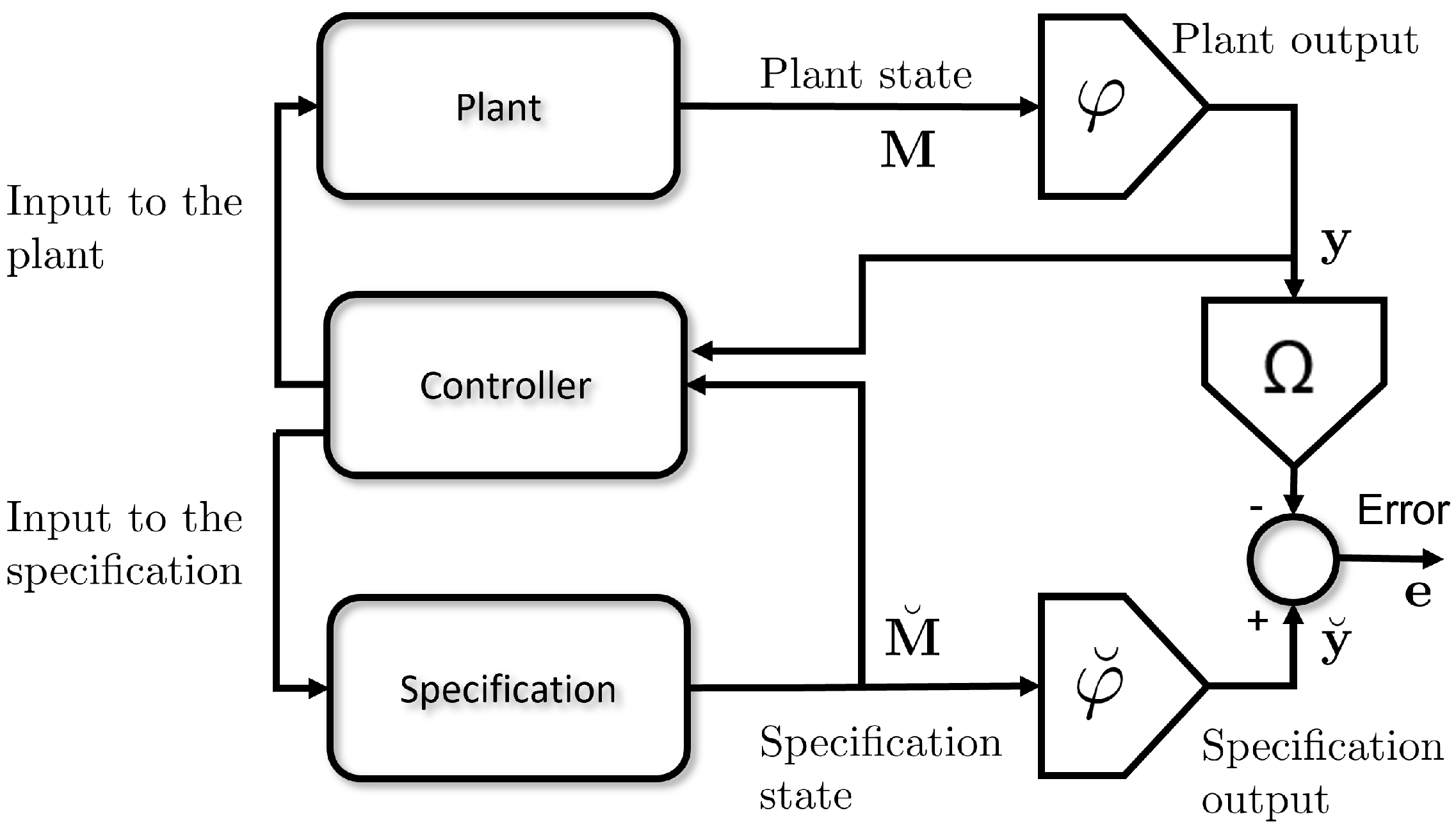
Regulation control is a paradigm, proposed for systems modeled by $IPN$, developed to induce sequences of output symbols on the system to be controlled, called the Plant. These sequences are specified in a high-level fashion by an $IPN$, called Specification (see, for instance [19,20,21]). Then, an $IPN$, named Controller, is designed for this purpose. Figure 2 shows a scheme describing the closed-loop system. In this, the controller indicates input symbols to the Plant transitions in order to make a selection of the Plant output ($\Omega ·\mathbf{y}$) to be equal to the Specification output ($\breve{\mathbf{y}}$), otherwise stated, to cause the output error $\mathbf{e}=\breve{\mathbf{y}}-\Omega ·\mathbf{y}$ to be null. For this, the controller has access to the complete marking of the Specification ($\breve{\mathbf{M}}$), since the controller and the Specification are implemented in the same hardware, but it only has access to output signals from the Plant ($\mathbf{y}$), since only this information is available through the sensors connected to the controller hardware. In addition, the controller stops the Specification when the output error is not null. The Plant and Specification are formally defined as follows.

Definition 3.

The Plant is a safe live $IPN$, $Q=\langle \mathcal{N},M_0,{\Sigma }_I,{\Sigma }_{Id},{\Sigma }_O,{\lambda }_I$, ${\lambda }_{Id},\phi \rangle$, that models the discrete event system to be controlled. Two places cannot generate the same output symbol; moreover, input and output alphabets are disjointed.

Definition 4.

A Specification is a safe, live-state machine IPN. $\breve{Q}=\langle \breve{\mathcal{N}},\breve{M_0},\breve{{\Sigma }_I}$, ${\breve{\Sigma }}_{Id}$, ${\breve{\Sigma }}_O$, ${\breve{\lambda }}_I$, ${\breve{\lambda }}_{Id}$, $\breve{\phi }\rangle$, together with a function $\Omega :{\Sigma }_O\to {\breve{\Sigma }}_O\cup \left\{ϵ\right\}$ that relates output symbols from the Plant to Specification output symbols. Each transition of the Specification has a unique identity symbol that is different from those of the Plant.

Methodologies for modeling automated manufacturing systems as $IPN$ have been proposed in [19,21]. Moreover, a methodology for designing $IPN$ specifications has been presented in [34], in which the designer only provides a high-level description of what he wants to observe from the Plant.

Definition 5.

A regulation controller is a safe $IPN$, $\widehat{Q}=\langle \widehat{\mathcal{N}},{\widehat{M}}_0,{\widehat{\Sigma }}_I,{\widehat{\Sigma }}_{Id}$, ${\widehat{\Sigma }}_O,{\widehat{\lambda }}_I,{\widehat{\lambda }}_{Id}$, $\widehat{\phi }\rangle$, fulfilling ${\widehat{\Sigma }}_{Id}\cap {\Sigma }_{Id}=\varnothing$ (i.e., plant transitions do not share their identity symbols with controller transitions). The closed-loop system is defined as the $IPN$$Q^{cl}=Q\parallel \breve{Q}\parallel \widehat{Q}$.

The regulation control problem consists of the synthesis of a controller that enforces the closed-loop system to exhibit the following behavior:

• if the output error is not null, then all the Specification transitions are disabled, and any fireable sequence drives the Plant to a marking where the output error is null;
• if the output error is null, then all the Plant transitions are disabled, but none of the Specification transition is disabled by the controller.

A synthesis method for computing such controller was presented in [20]. This method consists of the following three steps:

1.

A marking mapping $\Pi$ is computed, which relates each specification marking ${\breve{\mathbf{M}}}_k$ to a Plant marking ${\mathbf{M}}_k$, such that the output error is null, i.e., $\breve{\phi }{\breve{\mathbf{M}}}_k-\Omega \phi {\mathbf{M}}_k=\mathbf{0}$. Thus, if the Specification is at ${\breve{\mathbf{M}}}_k$, the Controller should drive the Plant to ${\mathbf{M}}_k=\Pi {\breve{\mathbf{M}}}_k$. The mapping $\Pi$ is computed by a linear integer programming problem (LIPP) that minimizes the number of firings between the plant markings (described by Parikh vectors $\overrightarrow{{\sigma }_k}$), subject to $\breve{\phi }=\Omega \phi \Pi$, $\Pi {\breve{\mathbf{M}}}_0={\mathbf{M}}_0$, $\Pi \breve{\mathbf{C}}\overrightarrow{\breve{t_k}}=\mathbf{C}\overrightarrow{{\sigma }_k}$ for all $\breve{t_k}\in \breve{T}$, and the entries of $\Pi$ and vectors $\overrightarrow{{\sigma }_k}$ are non-negative integers.

2.

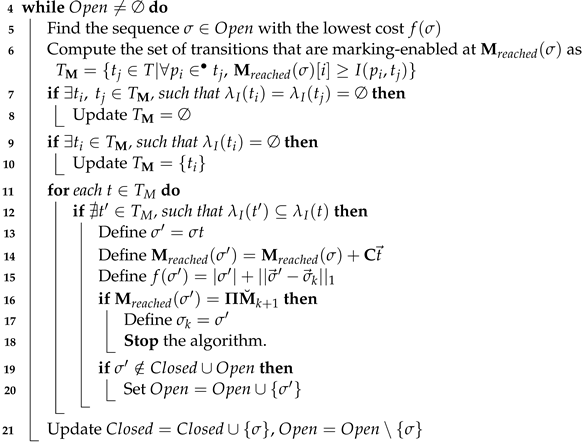
For each specification transition ${\breve{t}}_k$, such that ${\breve{\mathbf{M}}}_k[{\breve{t}}_k>{\breve{\mathbf{M}}}_{k+1}$, for some reachable ${\breve{\mathbf{M}}}_k$, a fireable controllable Plant sequence ${\sigma }_k$ is computed, such that $\Pi {\breve{\mathbf{M}}}_k[{\sigma }_k>\Pi {\breve{\mathbf{M}}}_{k+1}$. Thus, if ${\breve{t}}_k$ is fired in the Specification, reaching ${\breve{\mathbf{M}}}_{k+1}$, then the  Controller must induce the firing of ${\sigma }_k$ to reach $\Pi {\breve{\mathbf{M}}}_{k+1}$, so the output error becomes null. This is performed by the $A^{*}$ Algorithm 1, which computes a sequence with the minimum length that drives the Plant from $\Pi {\breve{\mathbf{M}}}_k$ to $\Pi {\breve{\mathbf{M}}}_{k+1}$. In the algorithm, the starting node is the empty sequence ${\sigma }_{ϵ}$; next, for each new node $\sigma$, the cost function is defined as $f\left(\sigma \right)=\left|\sigma \right|+\left|\right|\overrightarrow{\sigma }-{\overrightarrow{\sigma }}_k{\left|\right|}_1$ (where $\left|\right|•{\left|\right|}_1$ denotes the 1-norm), and the reached marking ${\mathbf{M}}_{reached}\left(\sigma \right)$ is computed (i.e., $\Pi {\breve{\mathbf{M}}}_k[\sigma >{\mathbf{M}}_{reached}\left(\sigma \right)$). Some conditions are included to ensure controllability (lines 7–10 and 12).

3.

Finally, an $IPN$ controller $\widehat{Q}$ is built, which enforces the previously computed Plant sequences ${\sigma }_k$, through the indication of Plant input symbols, when the corresponding specification transitions ${\breve{t}}_k$ have been fired.

Algorithm 1: Computation of a controllable sequence ${\sigma }_k$.

1 Input: $IPN$ Plant structure Q, starting marking $\Pi {\breve{\mathbf{M}}}_k$, ending marking $\Pi {\breve{\mathbf{M}}}_{k+1}$, Parikh vector ${\overrightarrow{\sigma }}_k$. 2  Output: Controllable sequence ${\sigma }_k$. 3  Initialize $Open=\left\{{\sigma }_{ϵ}\right\}$ and $Closed=\varnothing$. Set ${\mathbf{M}}_{reached}\left({\sigma }_{ϵ}\right)=\Pi {\breve{\mathbf{M}}}_k$. Set $f\left({\sigma }_{ϵ}\right)=\left|\right|{\overrightarrow{\sigma }}_k{\left|\right|}_1$.

The closed-loop system under the synthesized regulation controller is safe (i.e., bounded), since the Controller only constraints the behavior of the Plant, which is already safe. Moreover, the closed-loop system is live, since the Controller induces the occurrence of each computed sequence, which is fireable and controllable by construction, when the corresponding specification transition fires, and the Specification is live by definition.

4. RCPetri MATLAB^® App

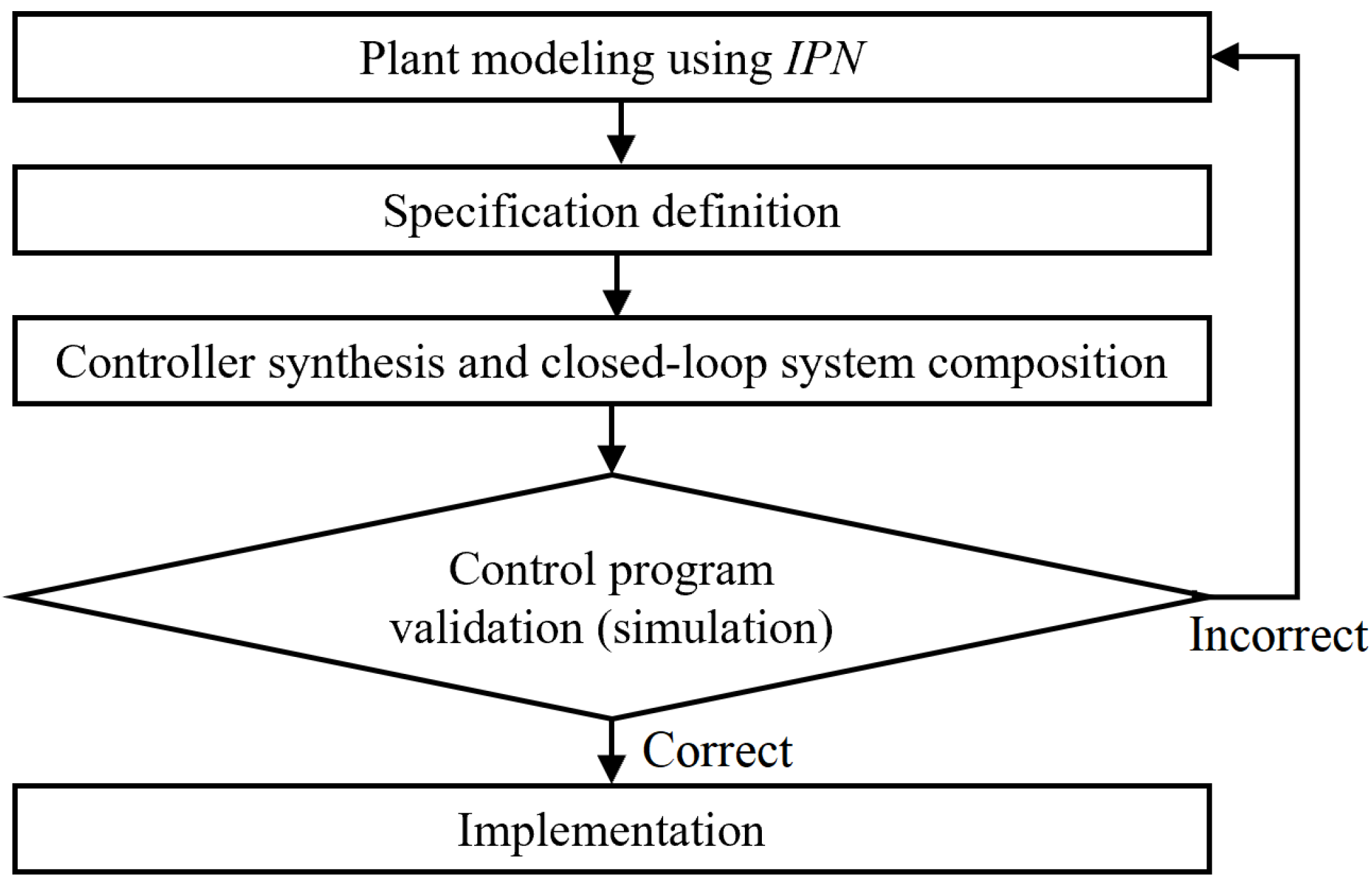
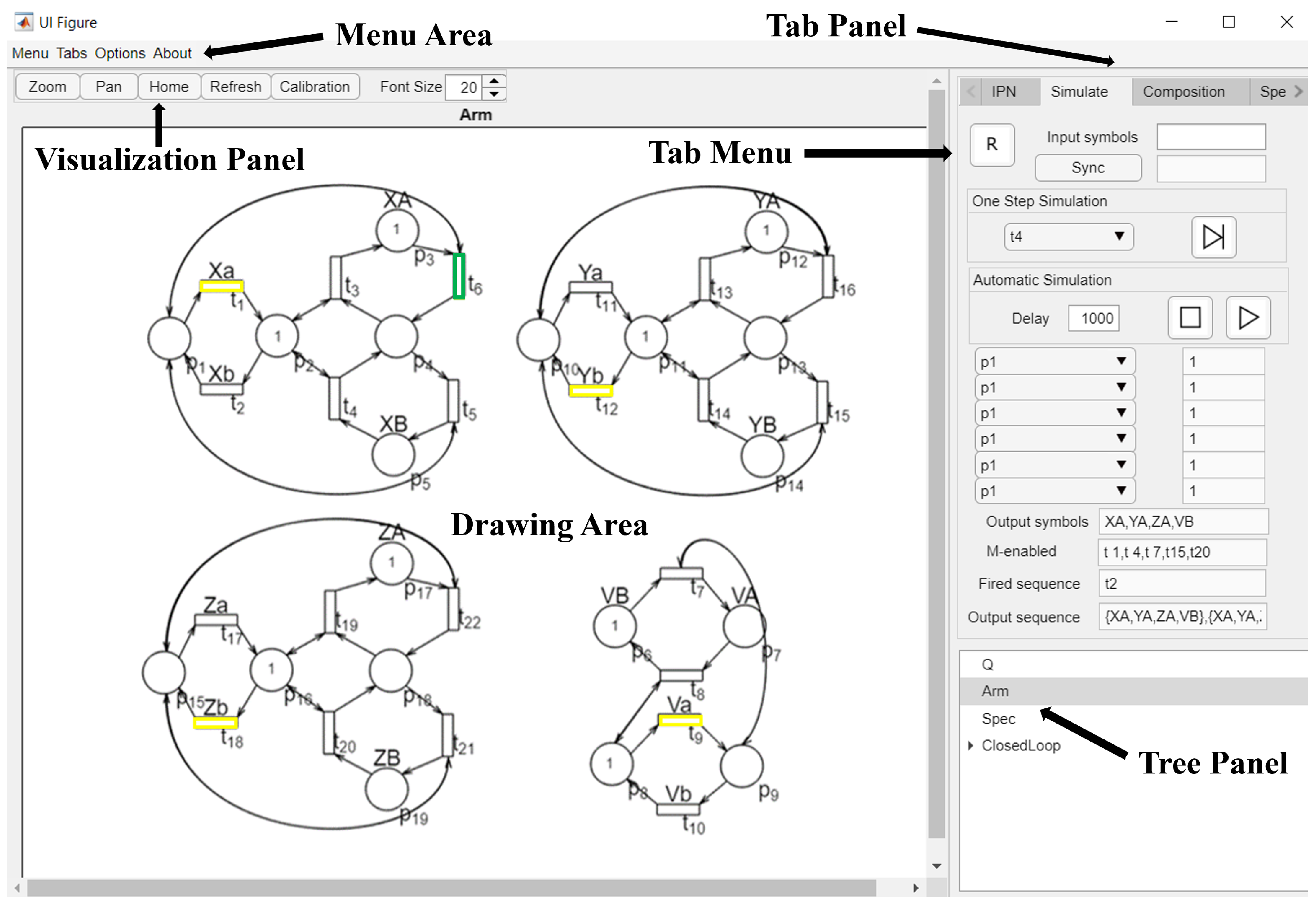
Figure 3 shows the steps that a practitioner should follow to implement the regulation control framework. The RCPetri MATLAB^®  app was designed to aid engineers to perform each of these steps. The app’s interface (shown in Figure 4) includes a main “Menu area”, a “Visualization panel”, a “Drawing area”, and a “Tab panel”. The app functionality is organized in Tabs, which can be accessed from the “Tab panel” and the “Tabs menu”.

4.1. Defining $IPN$ Models

The first step is to define an $IPN$ model in the “$IPN$ Tab”, by adding places and transitions to the “Drawing area”. Later, arcs can be defined by clicking on the “Arc icon” at the “Arc subtab” and then selecting the nodes to be connected through the arc. Identity and input symbols can be associated with selected transitions on the “Transition subtab”. Output symbols and tokens can be associated with selected places on the “Places subtab”. Arcs are defined by a set of control points, new control points are added to a selected arc by clicking on the button ( “o” ) (MATLAB^® apps can be slow. MathWorks does not currently provide a solution to speed up apps. In the case of RCPetri, the speed depends on the number of nodes and labels to be drawn. It is advised to use the “Zoom tool” to maintain the number of drawn nodes as small as convenient. Additionally, the “Menu Options” provides the possibility to avoid writing labels. Another issue in MATLAB^® apps is the mismatch between the cursor and axes coordinates. To correct this, press the “Calibration button” and next click at the center of the red cross).

Once an $IPN$ is drawn, a name must be given and the “Generate button” must be pressed. This will compute all the $IPN$ matrices as defined in Section 2, which are packed in a MATLAB^® struct variable with the name of the $IPN$ with the fields Draw (information for drawing the $IPN$), M0 (${\mathbf{M}}_0$), I (I), O (O), AO (${\Sigma }_O$), LP ($\phi$), AI (${\Sigma }_I$), LT (${\lambda }_I$), AID (${\Sigma }_{Id}$), and LTI (${\lambda }_{Id}$). This variable is accessible and editable from the MATLAB^® Workspace, and it is used for simulation, composition, and control synthesis. A struct variable containing a previously generated $IPN$ can be uploaded to the app, by using the “Load from WS button”.

Additionally, the “$IPN$ Tab” allows us to design $IPN$s in a modular way, by composing $IPN$s previously generated. However, the app does not currently allow us to define neither subnets nor subsystems. Thus, once a set of nets are composed, they integrate one monolithic $IPN$ system. The “Tree panel” at the right lower corner allows us to change the current$IPN$ by clicking on the name of the desired $IPN$.

4.2. Simulation

The “Simulate Tab” is used to simulate the current $IPN$ system. Before starting a simulation, the user must click on the reset button (“R”), in order to compute the initially enabled transitions. The simulation can be driven in three ways: by clicking on the enabled transitions on the drawing area, by selecting the transition to fire and pressing the “Step button”, or by pressing the “Play button”; in the last case, a randomly selected enabled transition will fire after a number of milliseconds specified by the user (“Delay”). Marking-enabled transitions are drawn in yellow, while enabled transitions are drawn in green (see Figure 4). External input symbols can be specified by the user at any time in the “Input Symbols” text field, symbols must be separated by commas (e.g., $a,b$ means the simultaneous indication of a and b). Drop down items allows us to select places, transitions and labels in order to visualize their values during the simulation.

4.3. Specification

The Specification $IPN$ can be defined by drawing and generating an $IPN$ (In this case, remember that each specification transition must have a unique identity symbol, which can be automatically generated in the subtab “IPN > Labels”). A more efficient option is to apply the specification generation algorithm of [34], implemented in the “Spec Gen Tab”, which translates a set of standard tables (named “Task table”, “Subtask table’,’ and “Shortcuts table”) into an $IPN$. These tables can be provided in the Book Editor app (which can be open directly from the “Spec Gen Tab”) or in an Excel file. 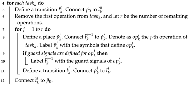To automatically compute the Specification $IPN$, the app applies two steps: first, the description of subtasks and shortcuts are substituted into the “Task table”; later, Algorithm 2 is applied to translate the “Task table” to an $IPN$.    

Algorithm 2: Building the $IPN$ Specification.

1 Input: Task table. 2  Output: $IPN$ model $\breve{Q}$ representing the Specification. 3 Define the place ${\breve{p}}_0$ with one token. Label ${\breve{p}}_0$ with the symbols that define the first operation.

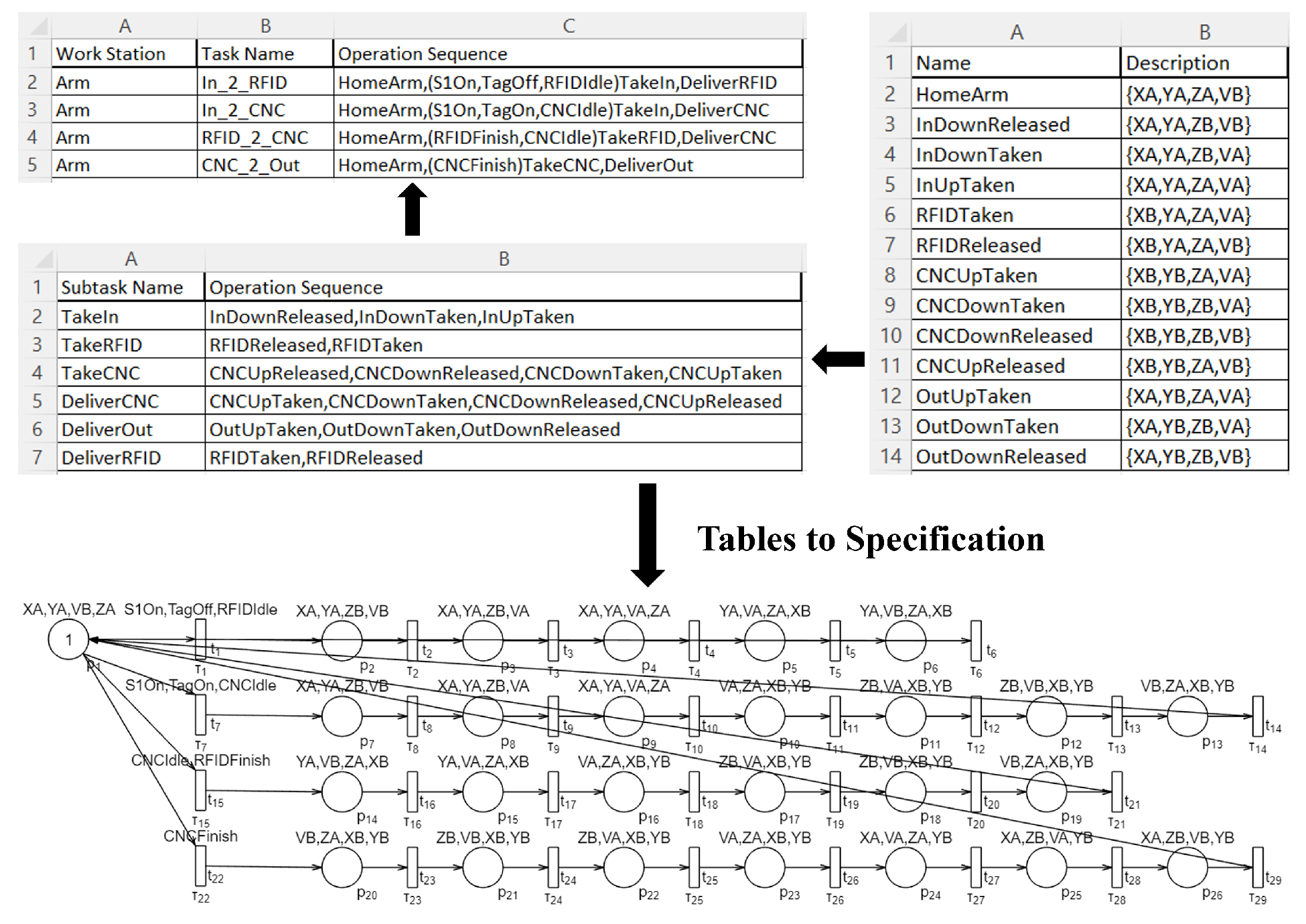
The “Task Table” must have three columns for the following:

1.

The workstation name (the Plant can be split in workstations).

2.

The task name (one workstation can perform several tasks).

3.

The operation sequence (each task is defined as a sequence of operations).

Each operation is described by the output symbols that are active when it is completed, these must be separated by commas and enclosed by curly brackets; round brackets can be used to define a set of guard signals that must be active to perform the operation (e.g., $(start,a)\{A,B,C\}$ denotes that both signals $start$ and a must be active to execute the operation $\{A,B,C\}$, characterized by the simultaneous activation of sensors A, B, and C). The first operation in all tasks must be the home position. For clarity, operations can be defined by using subtasksand shortcuts. Subtasks are defined in the “Subtasks table” as sequences of operations. Shortcuts are defined in the “Shortcuts table” as sets of output symbols. Figure 5 shows the tables in an Excel file that describe a specification for the $IPN$ arm model of Figure 4, notice that tasks include subtasks (e.g., $HomeArm$, $TakeIn$, etc.), which are defined using shortcuts. In an Excel file, the Tasks, Subtasks, and Shorcuts tables must be located in the first, second, and third sheets, respectively.

4.4. Control Synthesis

Once the Plant and the Specification are defined as $IPN$, a regulation controller can be computed in the “Controller Tab”, which implements the methodology introduced in [20] and resumed in Section 3, synthesizing an $IPN$ controller that enforces the occurrence of sequences ${\sigma }_k$ in the Plant to make the output error to be null. For this, the app modifies the Specification output labels (character # is added to each symbol) in order to distinguish them from the Plant output labels, and later, the labels mapping $\Omega$ is computed. The computation of the marking mapping $\Pi$ is performed by the MATLAB^® solver $intlinprog\left(\right)$. 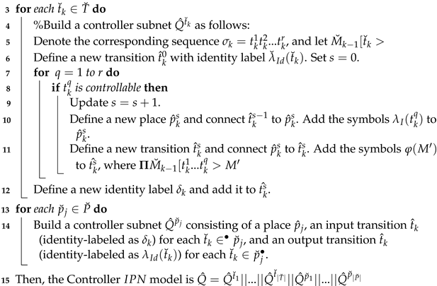Next, sequences ${\sigma }_k$ are computed with Algorithm 1. Finally, Algorithm 3 is executed to build the $IPN$ Controller. Moreover, the app generates the $IPN$ representing the control program ($\breve{Q}\left|\right|\widehat{Q}$) and the closed-loop system ($Q\left|\right|\breve{Q}\left|\right|\widehat{Q}$).   

Algorithm 3: Building the $IPN$ Controller.

1 Input: Plant Q. Specification $\breve{Q}$. Matrix $\Pi$ and sequences ${\sigma }_k$. 2 Output: $IPN$ model $\widehat{Q}$ representing the Controller.

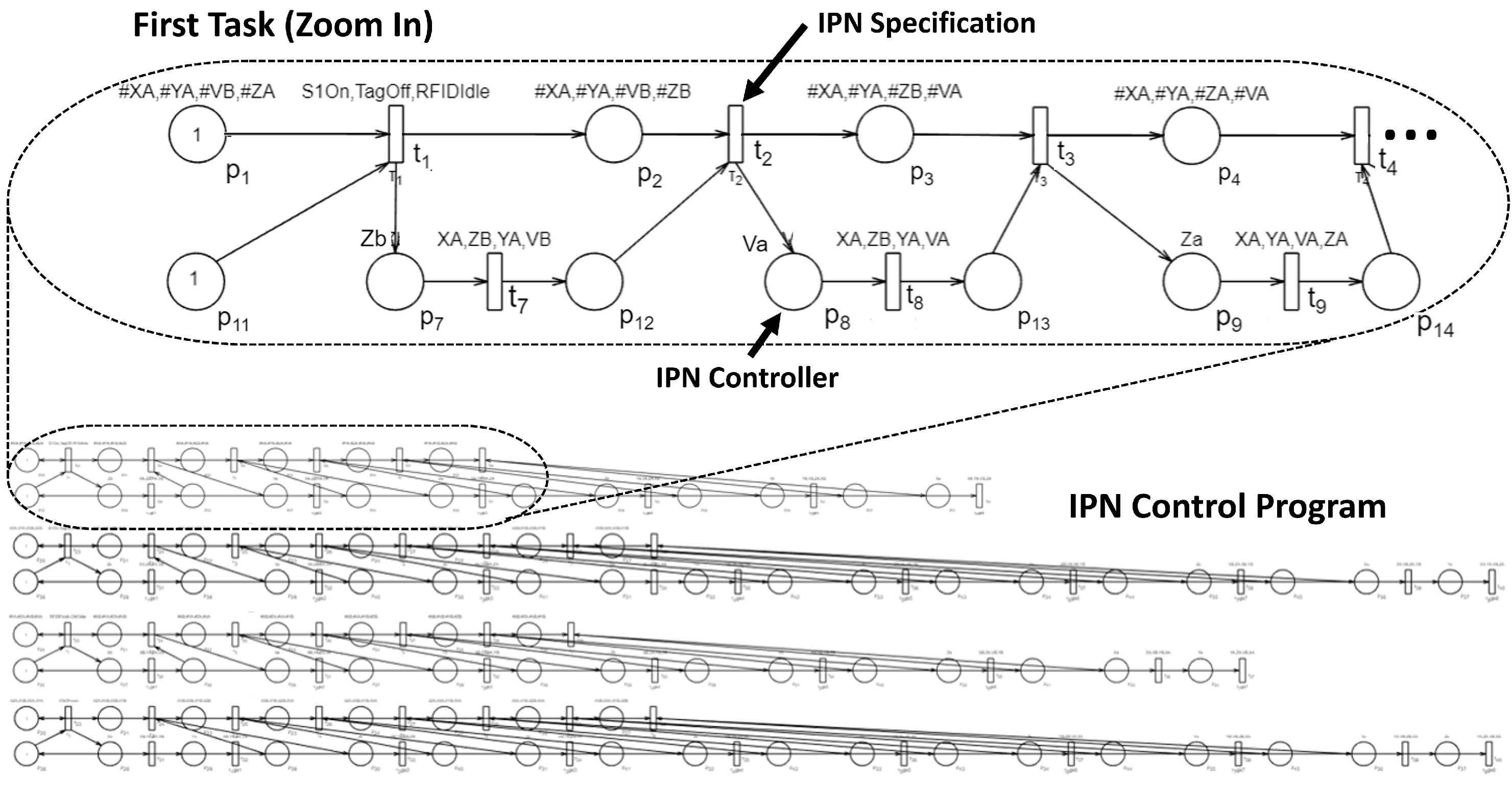
Example 2.

Figure 6 shows the automatically generated $IPN$ control program (i.e., the synchronization of Specification and Controller) for the Plant of Figure 4 and the Specification of Figure 5. Let us explain the behavior of the closed-loop system. For this, keep in mind that the $IPN$ Plant output symbols are read by the $IPN$ control to enable control transitions, and vice versa. At the initial state, the Plant provides the sensor signals $\{XA,YA,VB,ZA\}$ (operation HomeArm at the Specification tables). The first task (In_2_RFID) starts when the guard signals $\{S1On,TagOff,RFIDIdle\}$ are simultaneously active, leading to the firing of the control transition $t_1$, removing tokens from $p_1$ and $p_{11}$ and marking control places $p_2$ and $p_7$. The marking of the control place $p_7$ indicates the output symbol $Zb$, i.e., the controller commands the firing of a Plant transition labeled with $Zb$ ($t_{18}$ in Figure 4, which represents energizing coil b of the valve of actuator Z), allowing the Plant to reach the state characterized by the symbols $\{XA,YA,VB,ZB\}$ (i.e., the vertical actuator Z is down, corresponding to operation "InDownReleased"). These symbols coincide with those of the control transition $t_7$, becoming enabled and thus firing, moving a token from $p_7$ to $p_{12}$. Next, the control transition $t_2$ becomes enabled and it fires, removing tokens from $p_2$ and $p_{12}$ and marking the control places $p_3$ and $p_8$. Place $p_8$ indicates to the Plant to fire the transition labeled with $Va$ ($t_9$ in Figure 4, which represents energizing coil a of the valve of the suction cup), allowing us to reach the Plant state characterized by the following symbols: $\{XA,YA,VA,ZB\}$ (i.e., the suction cup V is active, corresponding to operation "InDownTaken"). These symbols coincide with those of the control transition $t_8$, becoming enabled and firing, moving a token from $p_8$ to $p_{13}$. Thus, the control transition $t_3$ becomes enabled and it can fire. This process is repeated until the first task is executed, and then the closed-loop system (both the Plant and the control program) returns to the initial state.

4.5. PLC Code Generation

For implementation, the $IPN$ control program ($\breve{Q}\left|\right|\widehat{Q}$) can be translated to PLC code in the “PLC Code Tab”. Two languages are supported, Instruction List (IL) and Structured Text (ST). In both cases, the application generates the code in a .txt file that is saved in the current MATLAB^® folder. The user can specify the input/output PLC ports for each symbol by means of a “Symbols Table”, which is provided by either the Book Editor app table or an Excel file (in the fourth sheet). The table format in both cases is equal, having four columns: input symbol, input port address, output symbol, and output port address.

Let us explain the translation algorithm. Each place $p_i$ of the $IPN$ program is associated with a memory bit ‘M1x’, where x represents the number i. First, a reset button is added, which sets the memories associated with the initially marked places to 1, and the other memories to 0. The second step codifies the dynamic behavior of the $IPN$ program, each $t_j$ is codified following the structure: If Precondition Then Postcondition, where the Precondition is such that all the memories associated with the input places of $t_j$ must be 1 and all the input ports associated with the symbols in ${\lambda }_I\left(t_j\right)$ must be active, and the Postcondition is that all the memories associated with the input places of $t_j$ are set to 0 and all the memories associated with the output places of $t_j$ are set to 1. Finally, each output port associated with an output symbol $o_i\in {\Sigma }_O$ is activated when the memory associated with a place in $\left\{p\right|o_i\in \phi \left(p\right)\}$ is 1.

4.6. Modbus TCP/IP and OPC UA

The app can synchronize input/output symbols with other software or hardware via Modbus TCP/IP or OPC UA. The app works in a similar way to Client. The “Modbus TCP/OPC-UA Client Tab” allows us to configure the connection. For this, a “Symbols table” must be provided, which relates the input/output symbols with the input/output ports (in the case of Modbus TCP/IP, the ports are numbered consecutively; in the case of OPC UA, the ports must be defined on the OPC UA server as Boolean variables). A Write/Read panel is included to help the user to check for the connection and the correct port assignation.

Once the app is linked, the “Simulate Tab” will allow us to simulate the $IPN$ synchronized with the server. For this, the “Reset button” (R) must be pressed and later the “Sync button” must be pushed. The input signals (input symbols) will be shown in a text field. Signals are read with a frequency specified at the “Refresh Delay text field” in the “Modbus/OPC-UA Client Tab” (delay between consecutive readings in $ms$). When an output symbol is generated during the simulation, this is immediately converted to a signal according to the symbols table and sent to the server.

5. Application Examples

In this section, three different examples are presented to illustrate different features of the RCPetri app, involving representative devices and automation systems: a pneumatic system, a process under logic control, and a robotic manufacturing system.

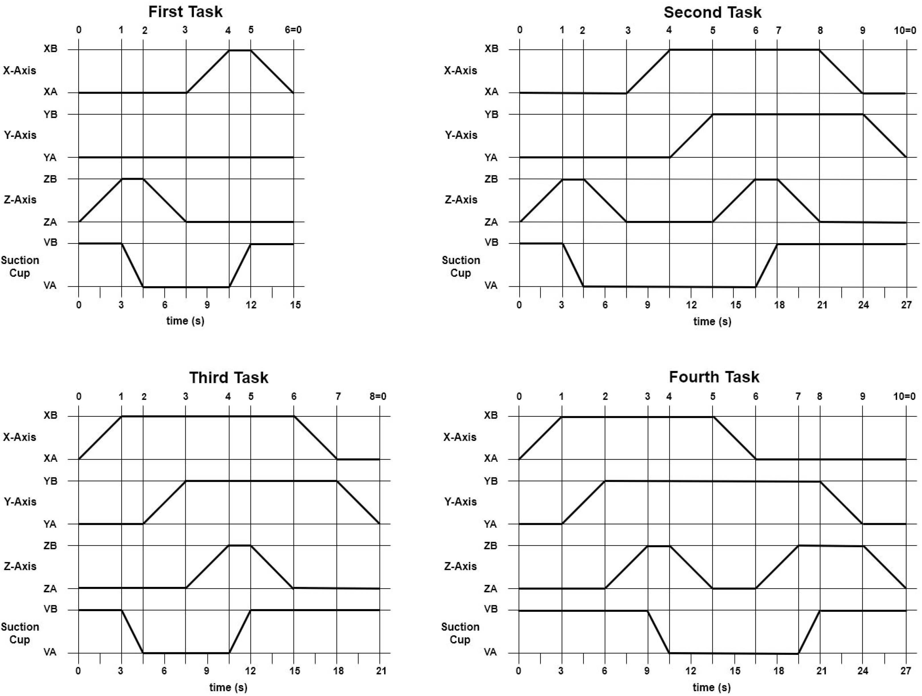
5.1. Pneumatic Arm

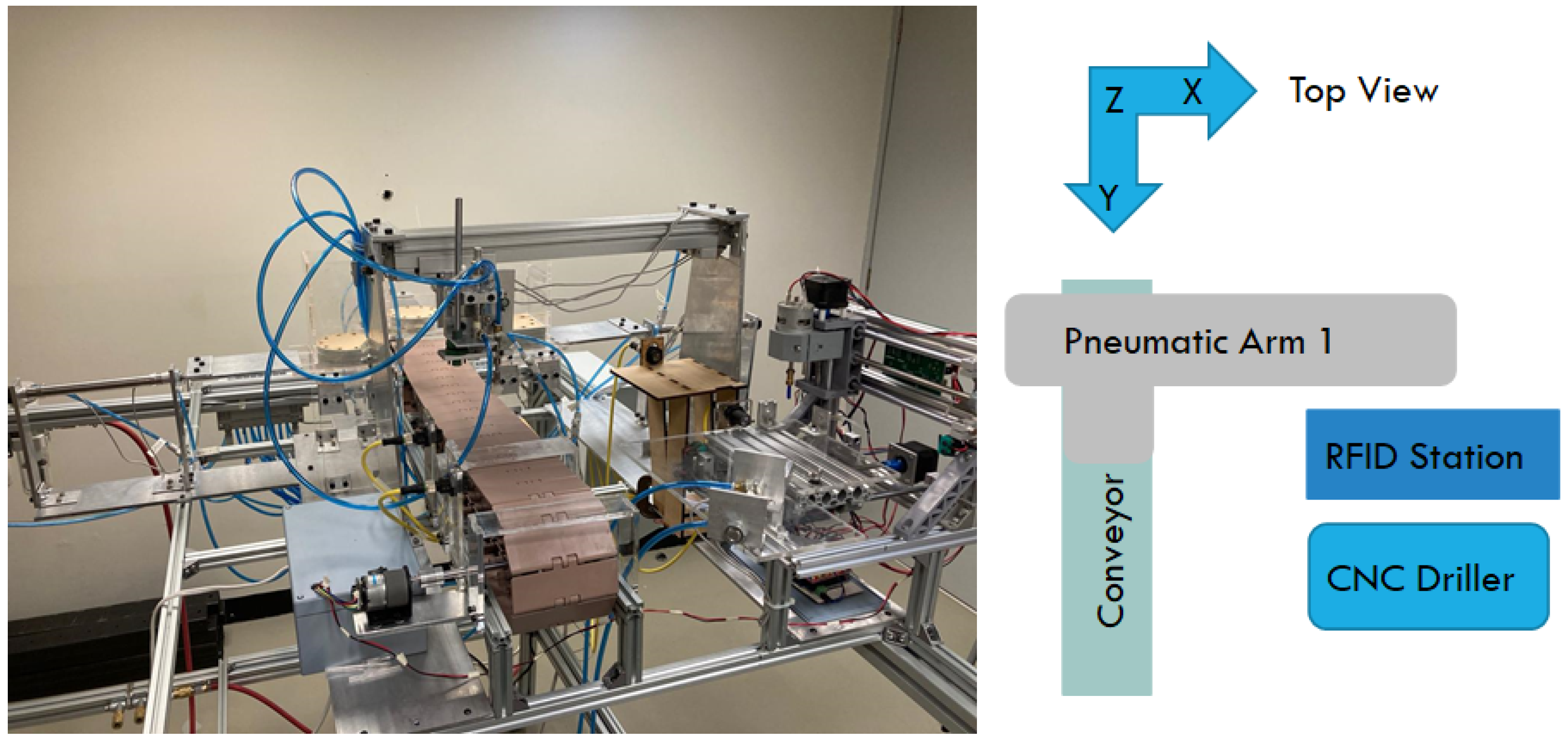
This example describes the application of the complete workflow of Figure 3 for the synthesis and implementation of a regulation controller for the electro-pneumatic arm with three degrees of freedom (3-DoF), as shown in Figure 7, which belongs to a small-scale manufacturing cell that assembles wood parts, named caps. According to the workflow, the first step is to obtain the Plant model. For this, the methodology of [19] was used, obtaining the $IPN$ depicted in Figure 4, which consists of four submodels, one for each double-effect pneumatic actuator and another for the suction cup.

The arm must perform four different tasks:

1.

If there is a cap at the conveyor’s $In$ position without a radio-frequency identification (RFID) tag, then the arm moves it to the RFID station (to attach a RFID tag to it);

2.

If the cap has a RFID tag, then the arm moves it to the computer numerical control (CNC) station (to drill 10 holes on it);

3.

If the RFID station has collocated a tag on a cap, then the arm moves the cap to the CNC station;

4.

If the CNC has drilled a cap, then the arm moves it to the conveyor’s $Out$ position.

This Specification was written in the tables depicted in Figure 5. For instance, the first task $In\_2\_RFID$ starts from the $HomeArm$ state, characterized by $\{XA,YA,ZA,VB\}$. This task is enabled by the signals $S1On$ (the cap is at the conveyor’s $In$ position), $TagOff$ (the cap does not have a RFID tag) and $RFIDIdle$ (the RFID station is available). When these are active, the subtask $TakenIn$ must be executed, defined as the operation sequence $InDownReleased$, $InDownTaken$ and $InUpTaken$, characterized by $\{XA,YA,ZB,VB\}$ (i.e., at the $In$ position, the suction cup is down and inactive), $\{XA,YA,ZB,VA\}$ (i.e., at the $In$ position, the suction cup is down and active) and $\{XA,YA,ZA,VA\}$ (i.e., at the $In$ position, the suction cup is up and active), respectively. The $IPN$ Specification depicted in Figure 5 was automatically computed with the app.

Next, the Controller, the control program, and the closed-loop behavior were computed with the “Controller tab”. The obtained control program is depicted in Figure 6 and described at the end of Section 4.4, which was translated to an IL PLC code with the “PLC Code tab”, obtaining 554 code lines. This code was used to implement the program in a PLC connected to the actual pneumatic arm, obtaining the desired closed-loop behavior, depicted in Figure 8. Let us remark that the engineer only provided the model of Figure 4 and the Specification tables of Figure 5, from this point, the app automatically transformed the tables to the $IPN$ model, automatically computed the $IPN$ control program of Figure 6, and automatically translated it to PLC code.

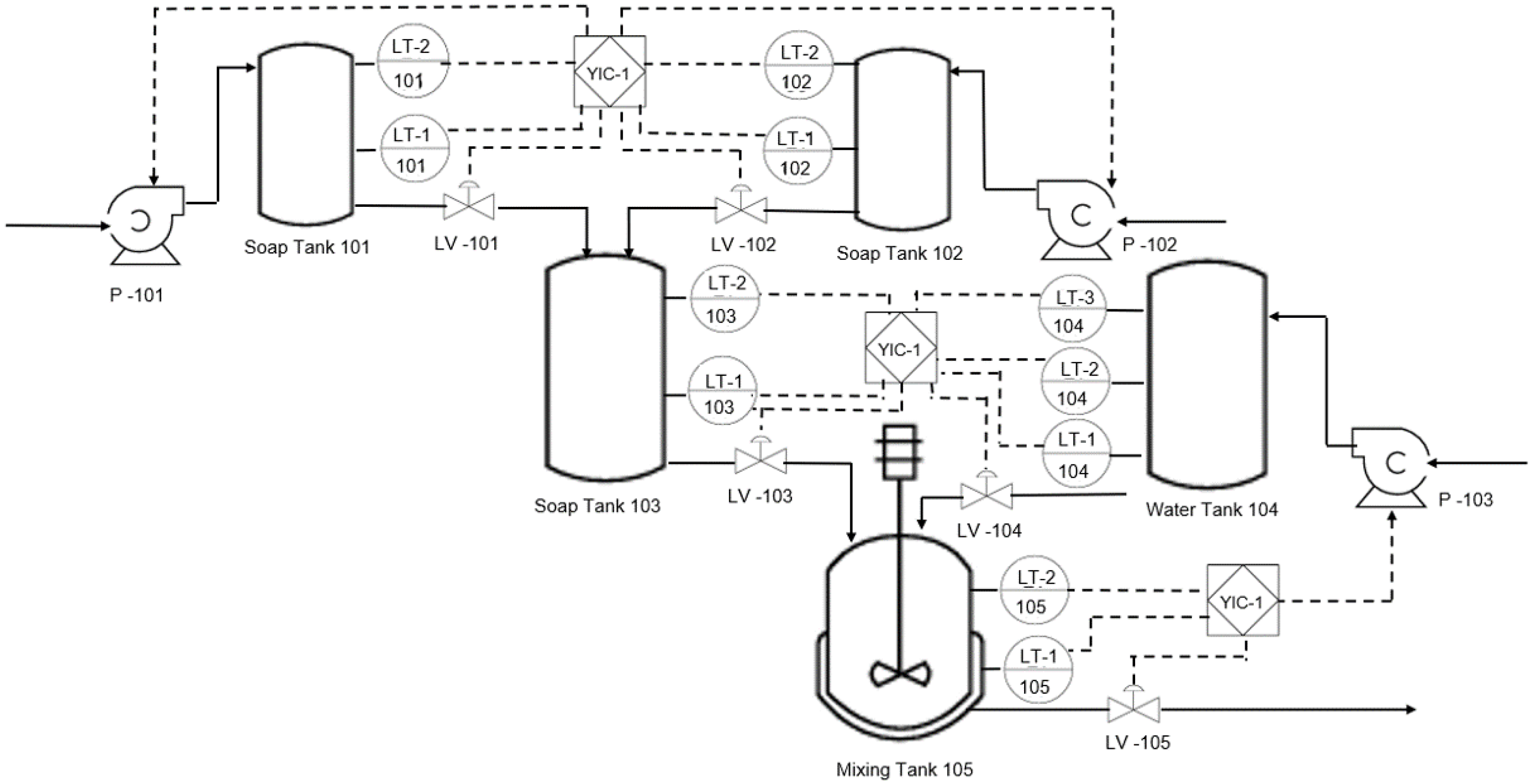
5.2. Tank Filling Process

This example exhibits the use of $RCPetri$ for the design and simulation of a logic controller for a tank filling process, simulated in the SCADA software LabVIEW^®, in real-time through the Modbus TCP/IP protocol.

The tank filling process considered here (adapted from [35]) is described by the piping and instrumentation diagram (P&ID) of Figure 9. The Plant model was obtained by using the industrial process modeling methodology presented in [21]. In this case, the sensors and actuators were modeled as two-state devices. Tank levels were model as variables with three discrete states (empty, low, high), excepting the water tank that also includes the state medium. These states can be inferred by level sensors LT, for instance, for Soap Tank 101, both sensor LT-1 and sensor LT-2 are inactive when the tank is at the empty state, named T1empty; sensor LT-1 is active and LT-2 is inactive at low state, named T1low; both sensors LT-1 and LT-2 are active at the high state, named T1high. In order to ensure controllability, additional input symbols $\delta$ were added to transitions representing a level change, these allow actuators’ controllable transitions to preempt level transitions ($\delta$ means waiting until the level change).

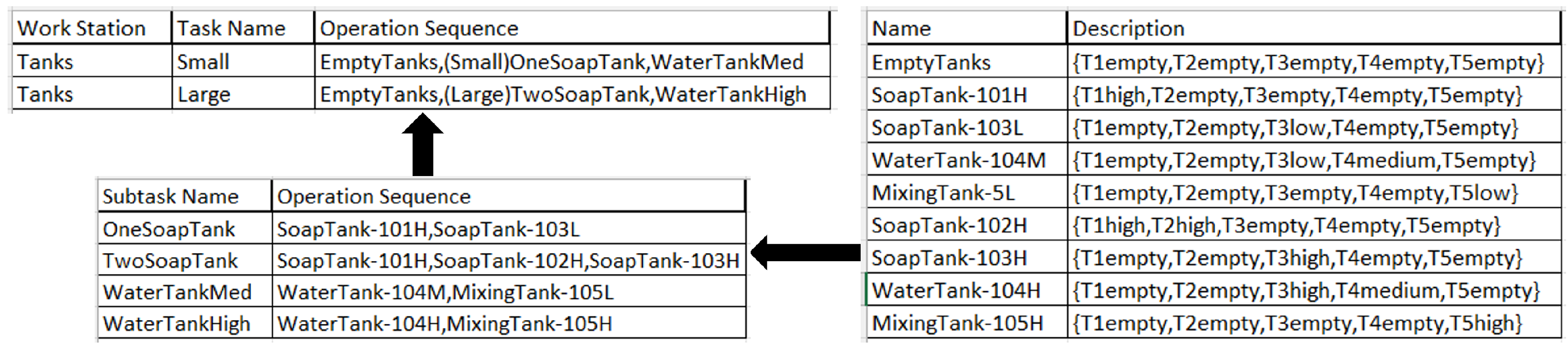
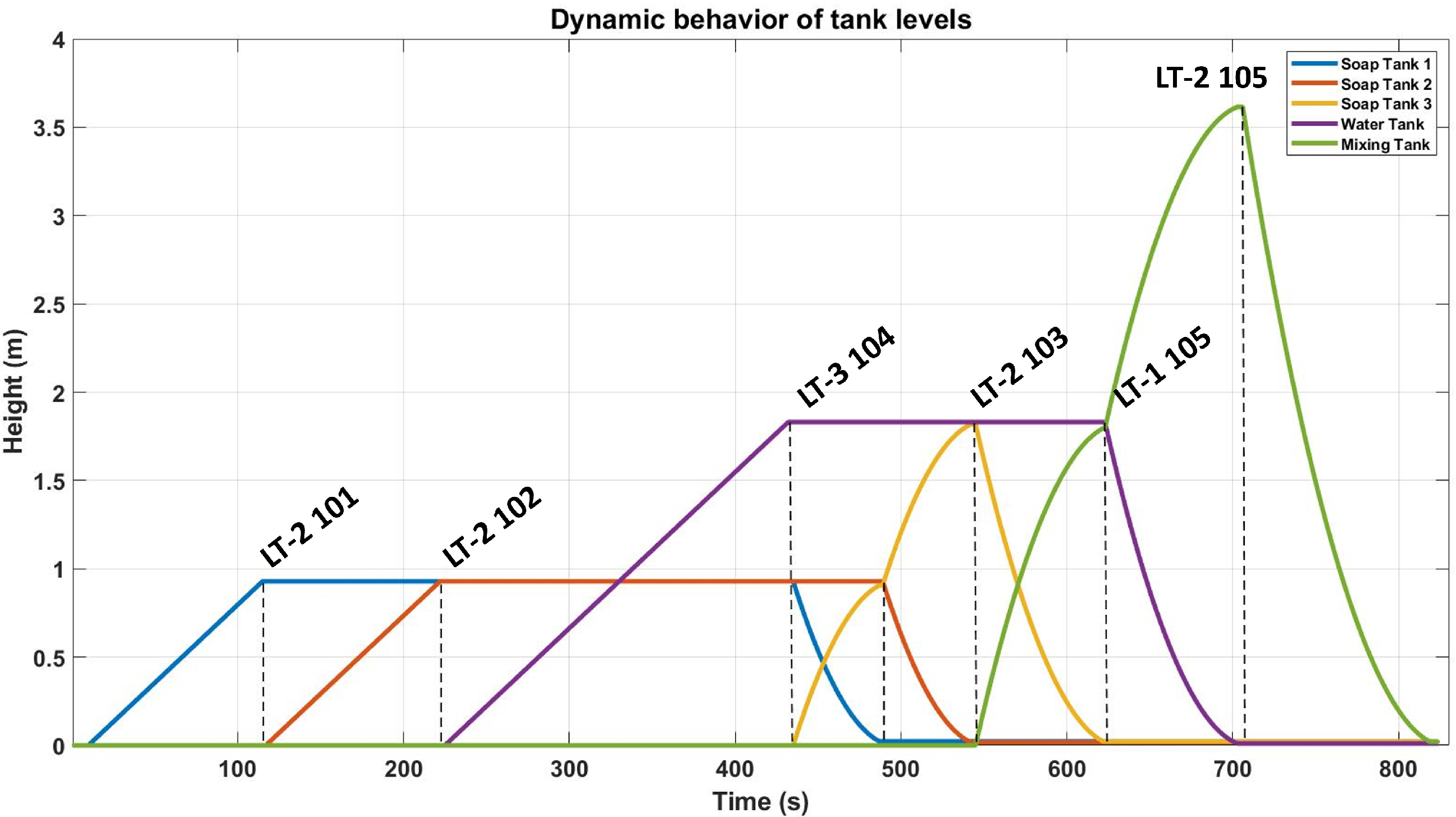
For the Specification, two different filling sequences were considered. In the first one, called “Small”, Soap Tank 103 is supplied by Soap Tank 101, the Water Tank 104 is supplied up to the middle level, next the fluids of Soap Tank 103 and Water Tank 104 are mixed in the Mixing Tank 105. In the second sequence, called “Large”, Soap Tank 103 is filled by both Soap Tank 101 and Soap Tank 102, while Water Tank 104 is filled up to the high level, then the fluids are mixed in the Mixing Tank 105. The Specification is described in the tables in Figure 10.

Once the $IPN$ Specification was synthesized, the Controller was computed. The $IPN$ closed-loop system is validated by simulation for implementation. The Plant was simulated on LabVIEW^® as a hybrid dynamical system (the tank levels evolve with continuous dynamics while pumps, valves and sensors evolve as state machines). Figure 11 depicts the tank filling dynamics during the “Large” sequence, under the control program being simulated in the app and connected through Modbus TCP/IP. Note that at the end of the filling of Tank 101, the control program allows the Tank 102 to start filling immediately. The simulation showed the effectiveness of the control program, as well as the interaction between $RCPetri$ and other software (in this case LabVIEW^®) in real-time. 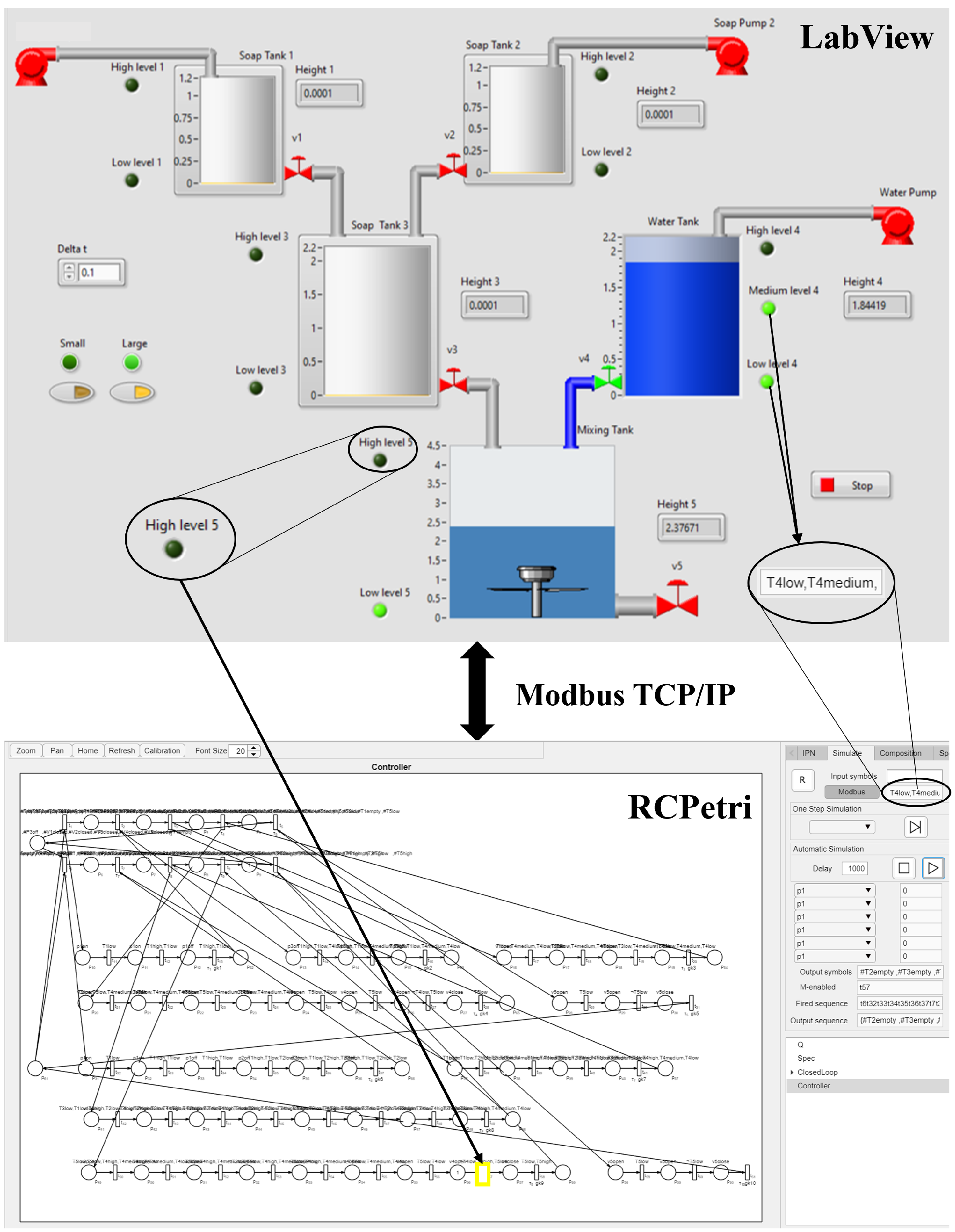Figure 12 shows the simulation of the Plant synchronized through Modbus TCP/IP with the $IPN$ control program, when the Water tank is filling the Mixing Tank during the “Large" task sequence.

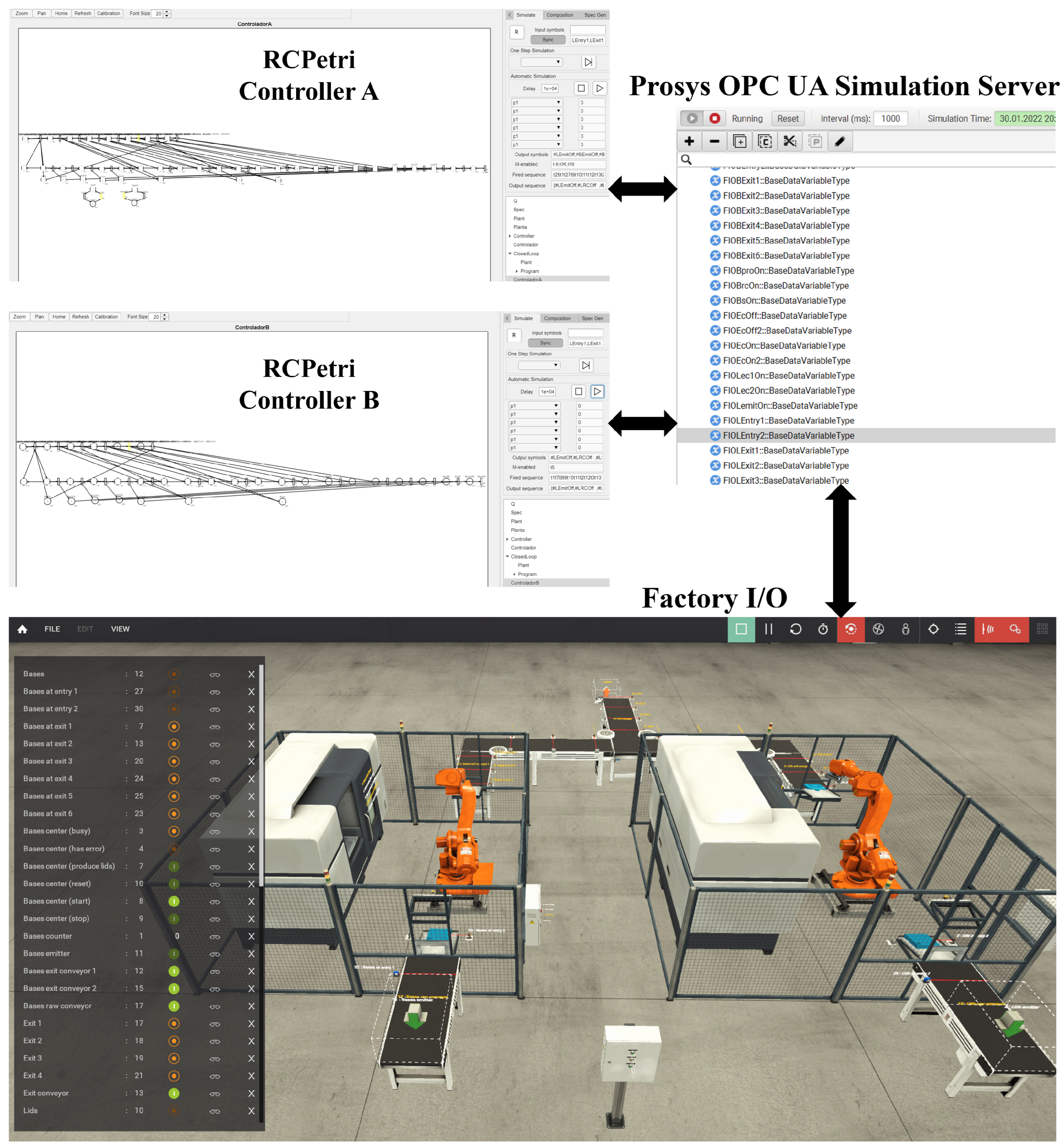
5.3. Robotic Manufacturing System

In this example, a manufacturing system composed of two robotic cells is considered. The objective is to show the effectiveness of $RCPetri$ for the implementation of a decentralized control scheme using the OPC UA protocol. For this, the Plant is simulated in the PLC training platform FACTORY I/O (see Figure 13), and two controllers are simulated in different app instances.

Each robotic cell is composed of a raw parts emitter ($Lemit$ and $Bemit$), an input conveyor belt ($Lrc$ and $Brc$), a robotic arm ($Ls$ and $Bs$), a CNC machine ($Lpro$ and $Bpro$), and two output conveyor belts ($Le{c}_1,Le{c}_2,Be{c}_1$ and $Be{c}_2$). In addition, both cells share an output conveyor belt $Ec$ and a manufactured parts remover $Rem$. Each robotic arm has a predefined program, which consists of moving a part from the entry to the CNC machine, wait for processing, and then moving the part to the exit. Each CNC machine can manufacture either bases or lids. Four sensors, $Le{n}_1,Le{n}_2,Be{n}_1$, and $Be{n}_2$, indicate the presence of raw parts at different positions on the input conveyors, while the sensors $Le{x}_1,\cdots ,Le{x}_6,Be{x}_1,\cdots ,Be{x}_6$ indicate the presence of manufactured parts on the output conveyors (Some sensors send a 1 as a logic signal when no object is present (sending a 0 in the opposite case), this can be handled in the app by using negation symbols ¬ in the output labels (e.g., $\neg Le{x}_1$)).

The Plant was modeled according to the methodology of [19]. Output labels were added to places representing actuator states, describing virtual sensors that allow the computation of controllable sequences. The system was required to perform lids production in the left cell and bases production in the right cell. This desired behavior was translated into two different $IPN$ Specifications, one Specification for the production of lids and the other for the production of bases. Later, each corresponding $IPN$ Controller was synthesized, obtaining a decentralized control scheme, as explained in [19].

Figure 13 displays the control simulation. Here, the Plant under the two synthesized control programs is running in FACTORY I/O. Both control programs are executed simultaneously, each one running in a different $RCPetri$ instance, synchronized through the OPC UA protocol. In this case, the Prosys OPC UA Simulation Server platform was used. This communication architecture made possible to effectively implement a decentralized control scheme.

6. Conclusions and Future Work

In this work, we have presented the main features of the RCPetri app, which allows us to efficiently and graphically define $IPN$ models, simulate $IPN$s, automatically generate $IPN$ specifications, automatically synthesize $IPN$ controllers using the regulation control approach, translate $IPN$ control programs into PLC code, and communicate with other software/hardware by using the Modbus TCP/IP and OPC UA protocols. In this way, the app can assist users to efficiently design and implement controllers through the complete control design workflow. In order to illustrate the features of the app, three examples were presented, being representative of common industrial automation systems: the design and PLC implementation of a controller for a pneumatic arm by applying the complete control design workflow; the design and simulation of a logic control of a filling tanks system, showing the synchronization of the $IPN$ controller simulation in the app with the tanks simulation in LabVIEW^®; finally, the design and simulation of a system composed of two robotic cells, showing the possibility to synchronize two instances of the app, each one controlling a different part of the Plant, with the Plant simulation in the software FACTORY I/O via the OPC UA protocol, obtaining a decentralized control architecture.

There are some aspects that have been identified as limitations that will be addressed in future releases. In particular, MATLAB^® apps tend to be slow when drawing several items, thus the drawing of large nets in the app becomes impractical. The current $IPN$ model does not integrate time information, which becomes relevant in some practical applications. Moreover, even if the app can be used to define and simulate unsafe nets, the current control synthesis algorithm cannot deal with unsafe nets. In future releases, methods for dealing with large nets and verifying specifications and controllers will be also included.