Abstract
To guarantee that a spectrometer can obtain effective solar spectral data, it is important that the two-dimensional turntable that carries the spectrometer tracks the sun with high accuracy for long time periods, such that the sun is always near the center of the field of view of the spectrometer. However, there is an offset lag problem for the tracking sensor, leading to an increase in the sun-tracking error and inaccuracies in solar spectrum data. To mitigate this problem, an on-axis tracking control algorithm—based on the orbital motion model—is proposed in this paper. First, the sun-tracking model of the spectrometer is established based on the coordinate transformation method, and the analytical relationship between the adjustment angle of the turntable and the solar vector in the orbit system is given by means of the inverse kinematics solution of the target model. Then, the predictive filtering algorithm of the target model is derived to acquire the target position, based on which, the on-axis tracking control algorithm of the spectrometer system is realized to compensate the offset lag and increase the sun-tracking accuracy. Finally, the simulation analysis and experimental verification were performed under the actual working conditions of an orbit. The simulation results demonstrate that the root-mean-square (RMS) of the target position deviation decreased from 2.08″ to 0.77″ after prediction filtering, and the RMS of the tracking error decreased from 7.14″ to 0.97″. The RMS of an orbit’s sun-tracking error decreased from 5.72″ to 1.43″ in the ground test. The simulation and experimental results verify that the algorithm proposed in this paper can improve the tracking accuracy of the spectrometer, providing a reference for the design of a spectrometer in orbit.
1. Introduction
A satellite-based spectrometer is on board all satellite platforms in a solar synchronous orbit. The solar spectral irradiance can be acquired by monitoring the influence of solar activity variation on the solar spectral radiation, providing data support for the field of meteorology [1]. To obtain effective spectral data, it is important that the spectrometer is able to track the sun for long time periods with a high accuracy. Because the incident angle of sunlight in orbit is greater than the effective field of the spectrometer, the spectrometer is mounted on a two-dimensional turntable to compensate for satellite orbital motion, allowing the mission requirements of the spectrometer to be achieved. Furthermore, an optical tracking sensor is mounted on the turntable, whose field of view is parallel to that of the spectrometer, and is employed to measure the deviation angle of the sun in the center of the field of view. The pointing and tracking of the sun by the spectrometer with high precision is achieved by combining data from the optical tracking sensor and the turntable position sensor.
When the tracking sensor processes and calculates the solar deviation angle, certain procedures take place, including image signal processing, target position extraction, and data transmission. Therefore, a time lag exists for the deviation angle, which leads to an overshoot when the spectrometer locks the sun in the center of the field of view and an impact on the bandwidth and phase margin of the control system during tracking [2,3]. In recent years, an on-axis tracking strategy has been widely used in photoelectric tracking systems by taking advantage of the fast computing ability of the controller to compensate for the time lag of the sensor, among which the predictive filtering algorithm and target motion model are two key elements that influence the control performance [4,5].
In terms of the predictive filtering algorithm, predictive control is combined with proportional-integral-derivative (PID) control, and the dual control strategy of the dynamic matrix control - PID (DMC-PID) cascade is adopted in reference [6] to improve the tracking accuracy and robustness of the system. The angle relationship between the position sensor and tracking sensor is employed in reference [7], taking the measurement data of both into consideration to design a time-lag compensator and improve the tracking performance of the system. However, the aforementioned algorithms cannot filter measurement noise. The current statistical model, based on the H∞ robust filtering algorithm, is established in reference [8], which first uses prediction and then fusion to solve the problems of miss distance lag and signal noise of the tracking sensor, where the filtering algorithm is relatively complex. The target state-space description method is adopted in the Kalman filter algorithm, and the process noise and measurement noise are introduced into the state model to describe the uncertainty of the tracking model, which can achieve the optimal estimation of the system state under white noise. Owing to its simple structure, low requirements for controller calculation, and energy storage capacity, this algorithm can be widely used in control systems under different working conditions [9,10,11,12]. In terms of the target model, the constant velocity (CV) model and constant acceleration (CA) model can be used when the system tracks non-maneuverable objects [13]. For maneuverable objects, the randomness of object tracking is estimated through different techniques, one of which is the Singer model, which hypothesizes that the target acceleration is an exponentially correlated stochastic process whose mean value is zero [14]. The acceleration value of the target is taken as the center in the current statistical model (CSM). The modified Rayleigh distribution function is employed to describe the probability distribution of acceleration, which can predict the position and speed of the maneuverable target, along with certain other parameters. This is the adaptive estimation of the mean value of acceleration in the Singer model [15]. CSM and other improved algorithms based on CSM are widely applied in engineering [16,17]. However, these systems will become unstable when faced with a weak maneuverable target such as the spectrometer with respect to the sun. [18].
In this study, in order to compensate for the impact of angular offset lag on the tracking performance and improve the accuracy of spectrum data, the target motion model of the spectrometer when tracking the sun, and the actual working condition were first obtained. Then a Kalman predictive filtering algorithm was proposed based on the motion model mentioned above and the actual control model was acquired. Finally, simulations and tests were conducted to verify the accuracy and effectiveness of the model and algorithm presented in this paper.
The remainder of this paper is organized as follows. The system composition and working principle of the spectrometer are described in Section 2. The angular motion model based on satellite orbital motion is established, the prediction filtering algorithm is deduced, and the control system model of spectrometer on-axis tracking is established in Section 3. Simulations and tests conducted to verify the models are presented in the paper in Section 4, and conclusions are drawn in Section 5.
2. Spectrometer System
The incident angle of sunlight on the working orbital plane of the spectrometer varies within a range of about 47° in a year, which is much larger than the effective field of view of the spectrometer. The spectrometer system is designed as shown in Figure 1, in accordance with the working characteristics of the spectrometer. Spectrometers with two certain spectra are mounted on a two-dimensional turntable. The deviation angle of the sun relative to the field of view of the spectrometer, which is caused by the orbital motion of the satellite, is compensated by adjusting the angular position of the turntable such that the optical axis of the spectrometer can be aligned with the sun in real-time. To realize the tracking of the sun, the two-dimensional turntable is directly driven by a permanent magnet synchronous motor (PMSM). The angular offset of the sun relative to the optical axis is measured by the tracking sensor, and the angular velocity of the turntable and the position of the rotor are measured using the absolute encoder to realize the vector control of the PMSM.
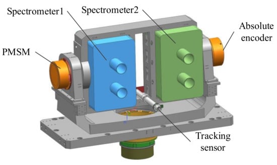
Figure 1.
Schematic of the spectrometer system.
When the spectrometer system is operating, the azimuth and pitch angular positions of the turntable are adjusted first to point at the sun, such that the sun lies in the effective field of view of the tracking sensor. Then, the two-axis angular positions are adjusted further in real-time to achieve sun tracking according to the measured angular offset. Only when the sun deviates from the center of the field of view of the spectrometer at a small angle can the two spectrometers obtain effective spectral data. The lower the tracking error, the better the performance of the optical system. Therefore, high-precision sun tracking and a stable two-dimensional turntable are imperative for the effective operation of the spectrometer.
The azimuth and pitch axes of the two-dimensional turntable are approximately orthogonal to each other, so the control of the two axes is independent. Vector control based on the magnetic linkage orientation of the rotor is adopted for the motor drive, and a typical control system for a single axis is shown in Figure 2. The control loop comprises a position loop, speed loop, and current loop, and a proportional-integral (PI) controller is adopted in each loop to realize closed-loop control. The current loop controls the acceleration of the turntable by controlling the stator current of the torque motor; its bandwidth is much larger than that of the speed loop and the position loop. The feedback speed is estimated from the position encoder using the cascading finite difference method (FDM) with a low-pass filter, and the speed loop ensures the stable operation of the turntable. The position loop obtains the angular offset from the tracking sensor to ensure that the turntable tracks the sunlight during closed-loop control [19].
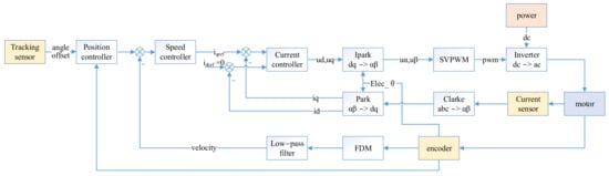
Figure 2.
Single-axis control principle of the spectrometer.
3. On-Axis Tracking Control Method based on the Orbital Motion Model
3.1. On-Axis Tracking Control Model
During the operation of the spectrometer, the turntable control is conducted in three steps: sun pre-pointing, locking, and tracking. The encoder data is employed for pre-pointing as feedback to realize the closed-loop position control. After the sun enters the optical field of view of the tracking sensor, the calculated angular offset is used to adjust the turntable to make the sun lie in the center of the field of view of the spectrometer and to keep the boresight axis of the spectrometer pointing to the sun. Owing to certain factors, such as the frame rate and image processing algorithm, the angular offset output from the tracking sensor lags behind its imaging time, which leads to the offset obtained by the control system lagging behind the current target position. This lag link is equivalent to adding a delay in the position loop, which has a negative influence on the stability and tracking accuracy of the system.
The on-axis tracking technology based on predictive filtering calculates the offset data at the current moment by predicting and estimating the lag offset to compensate for the influence of the data lag on the control system. On-axis tracking is proposed on the basis of composite control, which combines the data of the tracking sensor and the position sensor to obtain parameters such as the position and speed of the target. The on-axis tracking control model of the spectrometer system is shown in Figure 3. Firstly, the offset data Δθ(k-n) is fused with the encoder angle, where there is an artificial lag of n cycles θ(k-n) to obtain θref(k-n), which is the angular position of the sun with n lag cycles in the field of view of the spectrometer. Then, the fused data is processed with a predictive filtering algorithm to obtain the estimated value of the target position e_θref(k) and velocity e_speed(k) at the current moment. Finally, the target position and estimated velocity are used in the control system as the input of the position loop and as the feed-forward signal of the velocity loop, respectively, to realize equivalent composite control.
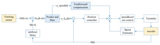
Figure 3.
The spectrometer on-axis tracking control model.
3.2. Target Motion Model
According to the control model, the estimation accuracy of the position and velocity of the predictive filtering algorithm, which are strongly dependent on the motion model of the target, directly determine the tracking accuracy and dynamic performance of the system. According to the working principle of the spectrometer, the rotation of the turntable compensates for the orbital motion of the satellite platform, ensuring that the sun is always in the center of the field of view. Therefore, to derive the motion model of the turntable, the sun vector needs to first be obtained under the orbital coordinate system through numerical calculations, and the azimuth and pitch angle of the turntable can be then calculated using the movement of the platform and the mounting position of the spectrometer on the satellite platform.
To accurately obtain the relationship between the target position and the rotation angle of the turntable, the coordinate systems are set up as shown in Figure 4. Firstly, an orbit coordinate system OO-XOYOZO is established. The origin OO is located at the center of mass of the satellite and the axis OOZO points to the center of the earth. OOXO is located in the orbital plane, in accordance with the flight direction of the satellite, and YO can be acquired through vector calculations. To simplify the motion model of the turntable, certain small errors can be ignored, such as the attitude error of the platform, various mounting errors, and the non-orthogonal errors of the turntable. Then, the satellite coordinate system OS-XSYSZS is defined, whose origin OS coincides with OO. The orbit system is coincident with the satellite system when there is no satellite attitude motion. Three angles—φ, θ, and ψ—are used to describe the three-axis attitude angles of the satellite system with respect to the orbit system. In terms of the turntable coordinate system OT-XTYTZT, the origin OT is located in the center of the image plane, and -OTYT represents the optical axis. The axes of the turntable system are parallel to those of the orbit system when there is no turntable motion [20].
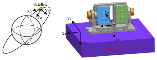
Figure 4.
Schematic of the coordinate systems.
According to the orbital parameters of the spectrometer, it can be seen that the incident angle of sunlight in the orbital plane varies by about 47 degrees within a year. Therefore, the data of four special days—the spring equinox, summer solstice, autumn equinox, and winter solstice—are calculated and simulated, which can basically reflect the range of the sun angle. Furthermore, the coordinates [Xs, Ys, Zs]T of the sun vector in the orbit system are obtained. According to the definition of the coordinate systems and the principle of coordinate transformation, the coordinate of the sun vector can be acquired in the turntable coordinate system, as shown in Equation (1).
where SC denotes the sun vector in the turntable coordinate system, whose theoretical value equals [0, −1, 0]T when the sun is in the center of the field of view of the tracking sensor. MOS denotes the transformation matrix used to describe the relative attitude of the satellite system with respect to the orbit system. MA and ME denote the transformation matrices of the local coordinate systems of the azimuth and pitch axes, respectively, when there is rotation with respect to the turntable system. Without a loss of generality, it is assumed that φ, θ, and ψ represent the rotating angles along the axes OOXO, OOYO, and OOZO of the satellite system, respectively, with respect to the orbital system. Matrix MOS is shown in Equation (2).
where cθ = cosθ, sθ = sinθ, and so forth.
When the rotation angles of the azimuth axis and the pitch axis are A and E, respectively, the transformation matrices are shown in Equations (3) and (4), and the analytical results for angles A and E can be obtained, as depicted in Equations (5) and (6).
Moreover, the sun vector data in the orbital system of the four special days (spring equinox, summer solstice, autumn equinox, and winter solstice) are substituted into the model above, and the azimuth angle A and pitch angle E of the turntable can be obtained as shown in Figure 5. According to the results, it can be seen that the resulting curves for the azimuth and pitch angles of the turntable are approximately sinusoidal.
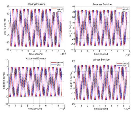
Figure 5.
Azimuth and pitch angle curves.
To reach a compromise between the fitting accuracy and the calculation capacity of the controller, the azimuth and pitch angles are fitted with the three-term sinusoids, as shown in Equation (7).
In Equation (7), A1 is the fundamental component representing the azimuth curve of the turntable when there is a cycle change of the sun vector in the orbit system. A2 and A3 denote the azimuth angles caused by nonlinear factors such as coordinate transformation and attitude control. In the four days shown in Figure 4, the amplitude of residual errors and periodicity of the azimuth and pitch angles in each orbit are basically the same when the fitting data is compared with that obtained from the satellite. Owing to the low speed of the satellite in orbit, the fitted data changes very slowly. Taking the azimuth curve in the first orbit of the spring equinox as an example, it can be seen that the standard deviation of the final error is about 0.02°. The fitting parameters are shown in Table 1, and the results are shown in Figure 6.

Table 1.
Fitting parameters in the first orbit of the spring equinox.
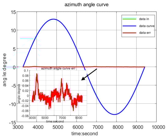
Figure 6.
Fitting results in the first orbit of the spring equinox.
3.3. Predictive Filtering Algorithm
The next step after obtaining the orbital motion model is to predict and estimate the target position. As a state optimal estimation algorithm in the time domain, the Kalman filter is advantageous in terms of its simple structure, high calculation speed, and high estimation accuracy; therefore, it was selected as the predictive filter algorithm of the control system for spectrometer on-axis tracking. According to the motion model of the turntable, the target angle of the turntable is approximated as the superposition of three sinusoids. The phase angle of each sinusoid is related to the moment when the spectrometer tracks the sun. Under the premise that working time is known, the amplitude, frequency, and phase angle of each sinusoid are updated by parameter injection from the ground before each orbit, which helps realize the adaptive function of the predictive filtering algorithm when working in different orbits every day.
To realize the practical engineering of the model, the angular position and velocity of the target angle are chosen as the system state. The angular positions are θ1 (t) = a1 ∗ sin (b1t + c1), θ2 (t) = a2 ∗ sin (b2t + c2), and θ3 (t) = a3 ∗ sin (b3t + c3). The corresponding angular velocities are ω1 (t), ω2 (t), and ω3 (t). The system state is shown in Equation (8), and the state-space expression of the control system is shown in Equation (9).
In Equation (9), w (t) is the process noise of the system, which mainly occurs owing to the errors of the target motion model. v (t) is the measurement noise of the system, which arises from the measurement noise of the encoder and tracking sensor. According to the physical interpretation, the process noise and measurement noise are not correlated with each other and are approximated as Gaussian white noise with a zero mean [21]. The discrete state-space expression of the system target model is derived as shown in Equation (11), where T is the sampling period of the system and Qk is the non-negative definite variance matrix of the process noise sequence W (k). Rk is the variance of the measurement noise V (k).
The initial state of the Kalman filter can be determined by the target model equation and the start time. The iterative process mainly includes two steps: prediction and correction. The covariance P(k + 1|k) of system state X(k + 1|k) can be predicted using the covariance P(k|k) of system state X(k|k), according to the state-space expression in Equation (11), as shown in Equation (13).
According to the predicted covariance matrix and the actual measured noise, the Kalman gain K(k + 1) can be calculated, and the predicted state and covariance are corrected with the Kalman gain. The state X(k + 1) of the system at time k + 1 is the output and the covariance matrix P(k + 1) at time k + 1 is calculated, as shown in Equation (14).
According to Equations (13) and (14), in addition to the target motion model, the reasonable estimation of the system noise and measurement noise, along with the design of the parameter matrices Qk and Rk, are the main factors that affect the performance of the Kalman filter [22]. For the spectrometer system analyzed in this paper, the measurement noise and sampling frequency of the encoder and tracking sensor are constant, which can be taken as the direct references for Rk selection. When the measurement noise increases, the Kalman gain becomes smaller and the reliability of the prediction filtering algorithm for the system measurement results decreases. The process noise mainly comes from the target model error caused by the platform attitude control error. The Qk matrix can be designed according to the platform attitude stability and other parameters since the dependence of the predictive status on the target model can be regulated by adjusting the elements in the Qk matrix. The elements in Qk are supposed to be eclectically selected. If the elements are too large, the prediction cannot work well. If the elements are too small, the predictive status would depend excessively on the target model, with the result that the algorithm may be divergent when there is a relatively large model error. When the process noise is relatively large, the impact of the target model noise on the predicted value can be reduced by increasing the Kalman gain.
4. Simulation and Tests
4.1. System Simulation and Result Analysis
The azimuth motion compensation of the turntable is taken as the simulation object. To verify that the on-axis tracking algorithm based on the orbital motion model can improve the sun-tracking performance of the spectrometer, a simulation experiment that combines the on-axis tracking algorithm based on the orbital motion model with the azimuth tracking system of the spectrometer was performed.
The simulation model and parameters are as follows. The model parameters in the first orbit of the spring equinox in 2020 are specified first, including the sun vector in the orbit system and the measured satellite attitude. The standard deviation of the attitude stability is assumed to be 0.002°/s, and the target motion model of the turntable is analyzed according to the aforementioned parameters. The simulation models of the tracking sensor and the position sensor are determined according to the selection of the spectrometer system. The refresh frequency of the tracking sensor is 40 Hz and the lag is 25 ms. The angular offset error is approximated as Gaussian white noise, whose standard deviation is about 1″. The refresh frequency of the position sensor is 1 kHz and the lag is 1 ms. The position measurement error is also approximated as Gaussian white noise whose standard deviation is about 1″. The driving control principle of the PMSM is shown in Figure 2, and the on-axis tracking control is finally established as shown in Figure 3. The system simulation time is 10 s. To simulate the process of guiding the sun into the center of the field of view, the offset is set to be about 0.05° when the sun is captured.
The parameters of the target motion model, including the amplitude, frequency, and phase, are substituted into the predictive filtering algorithm based on orbital motion. Figure 7 shows the difference between the predictive target position and the actual one, along with the difference between the calculated target position with the offset and the actual position. In the figure, “pos ref err kf” represents the difference between the actual target position and the predicted target position, and “pos ref err tracker” represents the difference between the actual target position and the calculated target position with the offset. The figure clearly shows that the RMS of the target position deviation is reduced from 2.08″ to 0.77″ when the predictive filtering algorithm based on the orbital motion model is introduced. The angular offset lag of the tracking sensor is compensated effectively by the algorithm, whose noise is filtered as well.
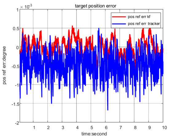
Figure 7.
Deviation curve of the target position.
The on-axis tracking control system is compared with the case in which the offset output of the tracking sensor is directly used as the position loop control. The angle tracking curves are shown in Figure 8a,b. In the figure, “track ref” represents the reference target position and “track fdb” represents the actual tracking position. “track err” is the difference between the reference tracking position and the actual position. The tracking error curves in Figure 8a,b are compared; it was found that the RMS of the tracking error is reduced from 7.14″ to 0.97″ and the standard deviation of the tracking error is reduced from 1.39″ to 0.96″ when the on-axis tracking control strategy is adopted. This verifies that speed feedforward compensation can be achieved by on-axis tracking control, with the precise speed prediction of the target model and the fluctuation of tracking error being reduced.
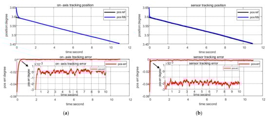
Figure 8.
(a) tracking position curve of on-axis tracking control; (b) tracking position curve of closed-loop simulation.
4.2. Tests
To verify the effectiveness and accuracy of the theory and simulation results, a spectrometer tracking experiment was set up in a laboratory environment to simulate the sun tracking of the spectrometer in orbit. The test environment is shown in Figure 9. A collimator is placed in front of the tracking sensor, at whose focal plane a strong light source is placed to simulate sunlight. It is important to ensure that the sunlight is always within the effective field of view of the tracking sensor throughout the tracking process. The spectrometer was placed on a six-degree-of-freedom (6-DOF) platform that simulates the motion of the satellite. The rotation range of the 6-DOF platform is larger than that of the turntable, using which the attitude control accuracy of the satellite platform in orbit could be simulated.
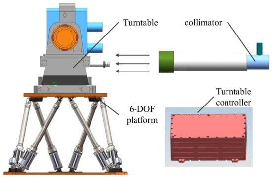
Figure 9.
Test environment for sun tracking.
The experimental parameters were in accordance with those of the simulation model. The 6-DOF platform must move according to the sun vector in the first orbit of the spring equinox in 2020 and simulate the stability of the satellite attitude control at the same time. The update frequency and error results of the tracking sensor and position sensor on the spectrometer were in accordance with those from the simulation model. The turntable controller could receive the injection parameters of the on-axis tracking control, and the light source tracking was realized by following the instructions of the on-axis tracking control model proposed in this paper or by directly using the offset of the tracking sensor.
First, the predictive filtering algorithm of on-axis tracking control was tested, and the results are shown in Figure 10. In the figure, “pos ref model” denotes the target position of the model, and “pos ref kf” denotes the target position calculated by the algorithm. “pos ref err” is the difference between the target position of the model and the predicted target position. The RMS of the measured target position deviation is 0.738″, which approximates the simulation result “pos ref err kf” in Figure 7. This indicates that the target motion model and the tracking sensor model in the simulation model are relatively accurate, and the delay of the tracking sensor can be effectively compensated by the predictive filtering algorithm with the angular offset filtered.
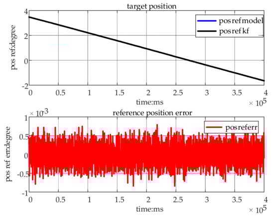
Figure 10.
Measured curve of the target position.
The closed-loop tracking test was conducted in the aforementioned environment. The output offset curves of the tracking sensor under the two known control strategies are shown in Figure 11. Under the two tracking strategies, the sun was always in the effective field of view of the tracking sensor, and sun tracking could be achieved.
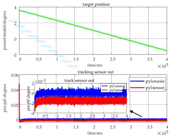
Figure 11.
Offset curve of sun tracking.
The angular tracking curves under the two control strategies are shown in Figure 12a,b. In the figures, “track ref” denotes the tracked target position and “track fdb” denotes the actual output position of the position sensor. “track err” represents the tracking error. In comparison to the simulation model, the measurement error of the encoder was introduced in the actual position in the test, which had little influence on the comparison of the tracking error under the two control strategies. Finally, the RMS of the tracking error was reduced from 5.72″ to 1.43″ after the adoption of the on-axis tracking strategy. These results show that the sun tracking error of the spectrometer can be effectively reduced by the on-axis tracking strategy based on the orbital motion model proposed in this paper.
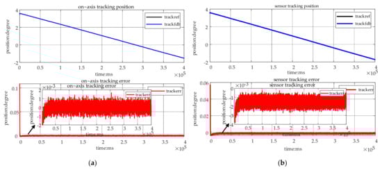
Figure 12.
(a) Closed-loop tracking position curve for on-axis tracking; (b) tracking position curve for offset position control.
5. Conclusions
The stability and precision of a spectrometer used for sun tracking for on-orbit work are extremely important. In this paper, coordinate transformation matrices are used to analyze the matrix transformation relationship of the spectrometer system, and the analytical relationship between the angular position of the turntable and the sun vector in the orbit system were obtained. Then, the target motion equation for sun tracking was acquired. Based on certain equations proposed above, an on-axis tracking control algorithm was derived and the target position and velocity were predicted and filtered, along with the simulation and ground tests. The results show that the RMS of the sun tracking error of the spectrometer was reduced from 5.72″ to 1.43″ after using the control algorithm proposed in this paper, which improves the accuracy of sun tracking and provides theoretical support for improving the on-orbit performance of the spectrometer system.
Author Contributions
Conceptualization, X.G.; methodology, X.G.; software, X.G. and X.Q.; validation, X.G. and X.C.; formal analysis, X.G.; investigation, X.G.; resources, C.Y.; data curation, X.G.; writing—original draft preparation, X.G.; writing—review and editing, B.H.; visualization, X.G.; supervision, C.Y. and Y.G.; project administration, C.Y. and Y.G.; funding acquisition, C.Y. All authors have read and agreed to the published version of the manuscript.
Funding
This research was supported by the National Natural Science Foundation of China, grant number 12103053.
Institutional Review Board Statement
Not applicable.
Informed Consent Statement
Not applicable.
Data Availability Statement
Not applicable.
Conflicts of Interest
The authors declare no conflict of interest.
References
- Li, Z.F.; Wang, S.R.; Huang, Y. High-Precision and Short-Time solar forecasting by space-borne solar irradiance spectrometer. Acta Opt. Sin. 2019, 39, 167–171. [Google Scholar]
- Bar-Shalom, Y.; Li, X.R.; Kirubarajan, T. Estimation with Application to Tracking and Navigation; Wiley: New York, NY, USA, 2001. [Google Scholar]
- Chodos, S.L. Track-loop bandwith, sensor sample frequency, and track-loop delays. In Proceedings of the SPIE Aerospace/Defense Sensing and Controls, Orlando, FL, USA, 30 July 1998. [Google Scholar]
- Xiong, Z.K.; Li, F.Y. Study on On-axis Tracking Algorithm of Modified Current Statistical Model. In Proceedings of the IEEE 2nd IAEAC, Chongqing, China, 25–26 March 2017. [Google Scholar]
- Lu, M.M.; Hou, R.M.; Ke, Y.F. Compensation method for miss distance time-delay of electro-optical tracking platform. J. Xi’an Jiaotong Univ. 2019, 53, 141–147. [Google Scholar]
- Yang, X.J.; Wang, Y.H.; Chen, E.R. The Study of DMC-PID Algorithm in the application of Photoelectric Tracking system. In Proceedings of the IEEE 3rd ICACTE, Chengdu, China, 20–22 August 2010. [Google Scholar]
- Yadegar, M.; Karami, F.; Nobari, J.H. A new control structure to reduce time delay of tracking sensors by applying an angular position sensor. ISA Trans. 2016, 63, 133–139. [Google Scholar] [CrossRef] [PubMed]
- Ji, W.; Li, Q.; Xu, B. Maneuvering targets state prediction based on robust H∞ filtering in opto-electronic tracking system. Signal Process. 2010, 90, 2002–2008. [Google Scholar] [CrossRef]
- Chen, D.D.; Yang, Y.; Pan, S. A new modified adaptive algorithm for time delay compensation of optoelectronic tracker. In Proceedings of the IEEE 8th IHMSC, Hangzhou, China, 27–28 August 2016. [Google Scholar]
- Zhou, Y.Y.; Wang, A.P.; Zhou, P. Dynamic performance enhancement for nonlinear stochastic systems using RBF driven nonlinear compensation with extended Kalman filter. Automatica 2020, 112, 108693. [Google Scholar] [CrossRef]
- Cortes, J.P.; Alzamendi, G.A.; Weinstein, A.J. Kalman Filter Implementation of subglottal Impedance-Based Inverse Filtering to Estimate Glottal Airflow during Phonation. Appl. Sci. 2022, 12, 401. [Google Scholar] [CrossRef]
- Zhang, H.W.; Xie, J.W.; Ge, J.A. Adaptive Strong Tracking Square-Root Cubature Kalman Filter for Maneuvering Aircraft Tracking. IEEE Access 2018, 6, 10052–10061. [Google Scholar] [CrossRef]
- Zhu, W.L.; Xu, Z.P.; Li, B. Research on the Observability of Bearings-only Tracking for Moving Target in Constant Acceleration Based on Multiple Sonar Sensors. In Proceedings of the IEEE Fourth International Symposium on Information Science and Engineering, Shanghai, China, 14–16 December 2012. [Google Scholar]
- Singer, R.A. Estimation Optimal Tracking Filter Performance for Manned Maneuvering Targets. IEEE Trans. Aerosp. Electron. Syst. 1970, 4, 473–483. [Google Scholar] [CrossRef]
- Zhou, H.R.; Jing, Z.L.; Wang, P.D. Maneuvering Target Tracking; National Defence Industry Press: Beijing, China, 1991. [Google Scholar]
- Wu, J.F.; Li, G.; Ma, F.Z. Research on Target Tracking Algorithm Using Improved Current Statistical Model. In Proceedings of the IEEE International Conference on Electrical and Control Engineering, Yichang, China, 16–18 September 2011. [Google Scholar]
- Cai, L.J.; Xu, X.T.; Liu, J.G. An IMM Algorithm for Tracking Maneuvering Targets Based on Current Statistical Model. In Proceedings of the IEEE 9th ISCID, Hangzhou, China, 10–11 December 2016. [Google Scholar]
- Wang, W.; Hou, H.L. An Improved Current Statistical Model for Maneuvering Target Tracking. In Proceedings of the IEEE Conference on Industrial Electronics and Application, Xi’an, China, 25–27 May 2009. [Google Scholar]
- Ha, D.H.; Kim, R. Nonlinear Optimal Position Control with Observer for Position Tracking of Surfaced Mounded Permanent Magnet Synchronous Motors. Appl. Sci. 2021, 11, 10992. [Google Scholar] [CrossRef]
- Huang, B.; Li, Z.H.; Tian, X.Z. Modeling and correction of pointing error of space-borne optical imager. Optik 2021, 247, 167998. [Google Scholar] [CrossRef]
- Rigators, G.G. A Derivative-Free Kalman Filtering Approach to State Estimation-Based Control of Nonlinear Systems. IEEE Trans. Ind. Electron. 2012, 59, 3987–3997. [Google Scholar] [CrossRef]
- Shi, T.N.; Wang, Z.; Xia, C.L. Speed Measurement Error Suppression for PMSM Control System Using Self-Adaption Kalman Observer. IEEE Trans. Ind. Electron. 2015, 62, 2753–2763. [Google Scholar] [CrossRef]
Publisher’s Note: MDPI stays neutral with regard to jurisdictional claims in published maps and institutional affiliations. |
© 2022 by the authors. Licensee MDPI, Basel, Switzerland. This article is an open access article distributed under the terms and conditions of the Creative Commons Attribution (CC BY) license (https://creativecommons.org/licenses/by/4.0/).