A Design of CGK-Based Granular Model Using Hierarchical Structure

Abstract

In this paper, we propose context-based GK clustering and design a CGK-based granular model and a hierarchical CGK-based granular model. Existing fuzzy clustering generates clusters using Euclidean distances. However, there is a problem in that performance decreases when a cluster is created from data with strong nonlinearity. To improve this problem, GK clustering is used. GK clustering creates clusters using Mahalanobis distance. In this paper, we propose context-based GK (CGK) clustering, which adds a method that considers the output space in the existing GK clustering, to create a cluster that considers not only the input space but also the output space. there is. Based on the proposed CGK clustering, a CGK-based granular model and a hierarchical CGK-based granular model were designed. Since the output of the CGK-based granular model is in the form of a context, it has the advantage of verbally expressing the prediction result, and the CGK-based granular model with a hierarchical structure can generate high-dimensional information granules, so meaningful information with high abstraction value granules can be created. In order to verify the validity of the method proposed in this paper, as a result of conducting an experiment using the concrete compressive strength database, it was confirmed that the proposed methods showed superior performance than the existing granular models.

1. Introduction

In In the field of artificial intelligence, an inference engine is a system component that applies logical rules to a knowledge base to infer new information, where the first inference engines are expert systems. Conventional expert systems comprise knowledge bases and inference engines. A knowledge base stores information about the actual world, and an inference engine applies logical rules to the knowledge base and new inferred knowledge. In this process, each piece of new information in the knowledge base can generate additional rules from the inference engine. These expert systems include fuzzy inference systems. Fuzzy inference systems are the core units of fuzzy logic system, which perform decision making as a basic task and employ logical gates such as “OR”, “AND”, and “IF-THEN” rules to generate the required decision rules.

Fuzzy inference systems are broadly divided into Mamdani and Sugeno types. Mamdani-type inference systems are created by combining a series of language control rules obtained from experts, and the output of each rule has a fuzzy set form. Because they have an intuitive and easily understood rule base, they are suitable in fields that employ expert systems that are created from the expert knowledge of humans, such as medical diagnoses. Sugeno-type inference systems are also called Takagi-Sugeno-Kang inference systems, and they use single output membership functions, which are a form of linear function, of a constant or an input value. Sugeno-type inference systems include a defuzzification process, and rather than calculating the center of a 2D region, they adopt a weighted average or weighted sum of several data points; hence, they have the advantage of exhibiting a higher computational efficiency than Mamdani-type inference systems. These fuzzy inference systems are used in various forecasting fields and are actively being studied [1,2,3,4,5,6,7,8,9]. A previous study [10] proposed a Fuzzy convolutional neural network (F-CNN) that combines fuzzy inference with a CNN to predict traffic flow, which is a core part of predicting traffic volume. Yeom [11] proposed adaptive neuro-fuzzy inference system (ANFIS), which has an incremental structure and adopts context-based fuzzy clustering. Parsapoor [12] proposed brain emotional learning-based fuzzy inference system (BELFIS) to predict solar activity. Kannadasan [13] proposed an intelligent prediction model for predicting performance indices such as surface roughness and geometric tolerance in computer numerical control (CNC) operations, which plays an important role in machine product manufacturing. Guo [14] proposed a model called backpropagation-based (BP) kernel function Granger causality, which adopts symmetry geometry to embed dimensions and fuzzy inference systems for time-series predictions; in addition, this model was utilized to examine the causal relationships between brain regions. Hwang [15] proposed a motion cue-based fuzzy inference system to predict the normal walking speeds of sudden pedestrian movements at the initial walking stage when the heel is lifted.

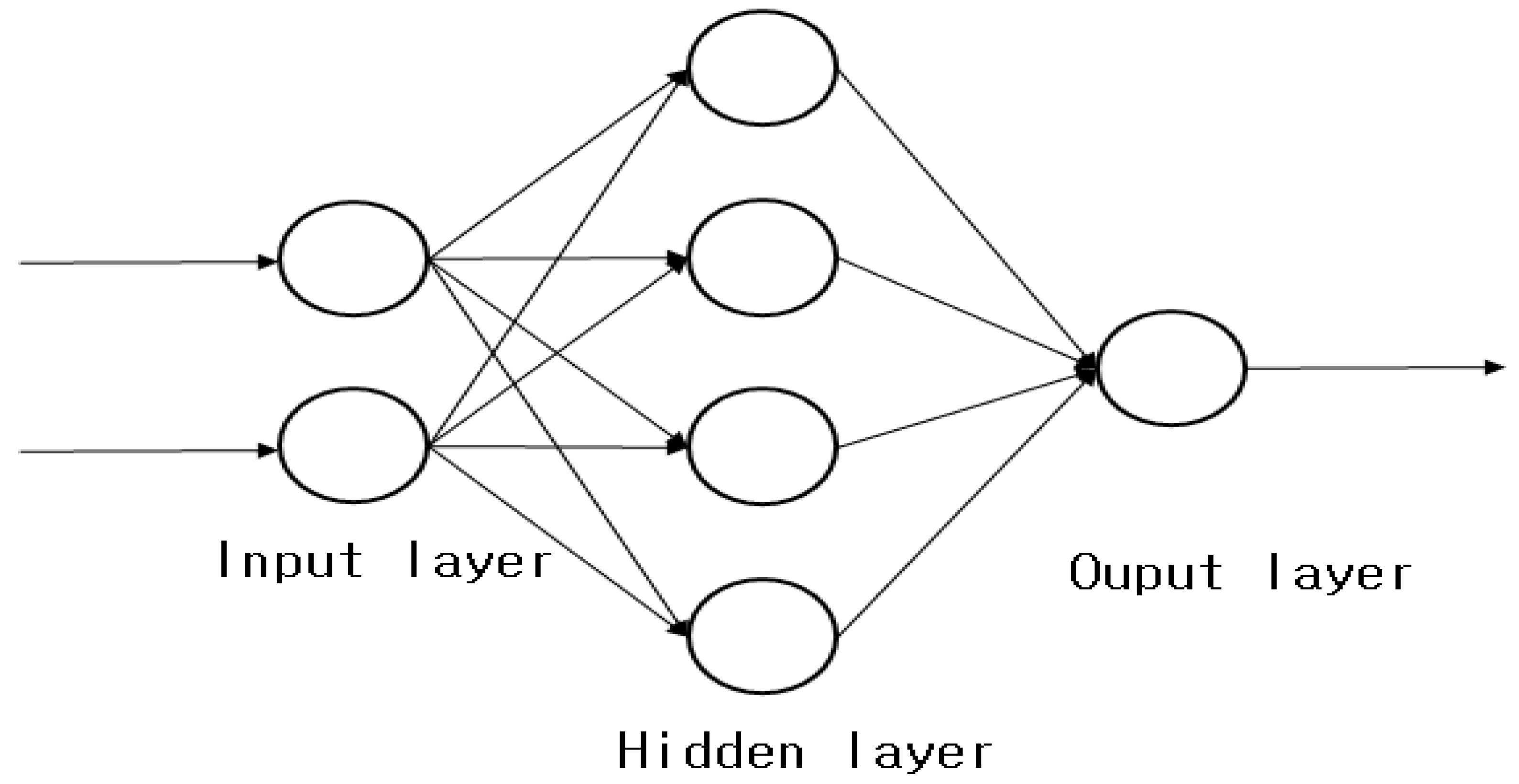
Neural network expert systems are expert systems that mimic human intelligence by combining artificial neural networks (ANNs) and expert systems. In conventional expert systems, human inference methods are designed using decision trees and logical inferences, while ANNs focus on the structure and learning capacity of the human brain and reflect this in their knowledge expression. If these two systems are combined, the process of deriving results can be confirmed by the expert system, while learning can be performed by the ANN without user intervention. Accordingly, it is possible to create a system that is capable of more effective inferences than existing individual systems. The following studies on such neural network expert systems have been conducted [16,17,18,19,20]. Liu [21] proposed recurrent self-evolving fuzzy neural network (RSEFNN), which adopts online gradient descent learning rules to solve brainwave regression problems in brain dynamics, to predict driving fatigue. Dumas [22] proposed prediction neural network (PNN), which is based on fully connected neural networks and CNNs, and is used for internal image prediction. Lin [23] proposed an embedded backpropagation neural network comprising two hidden layers for earthquake magnitude prediction.

The aforementioned fuzzy inference systems and ANNs have different processes and solve various prediction problems. In addition, studies are being conducted on solving problems by combining two or more different methods, rather than using one method. Inference systems that combine different methods are called hybrid systems, and the granular computing (GrC) [24,25] method is adopted as a method for constructing hybrid systems. GrC is a computing theory related to the processing of information objects, called “information granules” (IG), that occur during the process of extracting knowledge from data and information, as well as abstractifying the data.

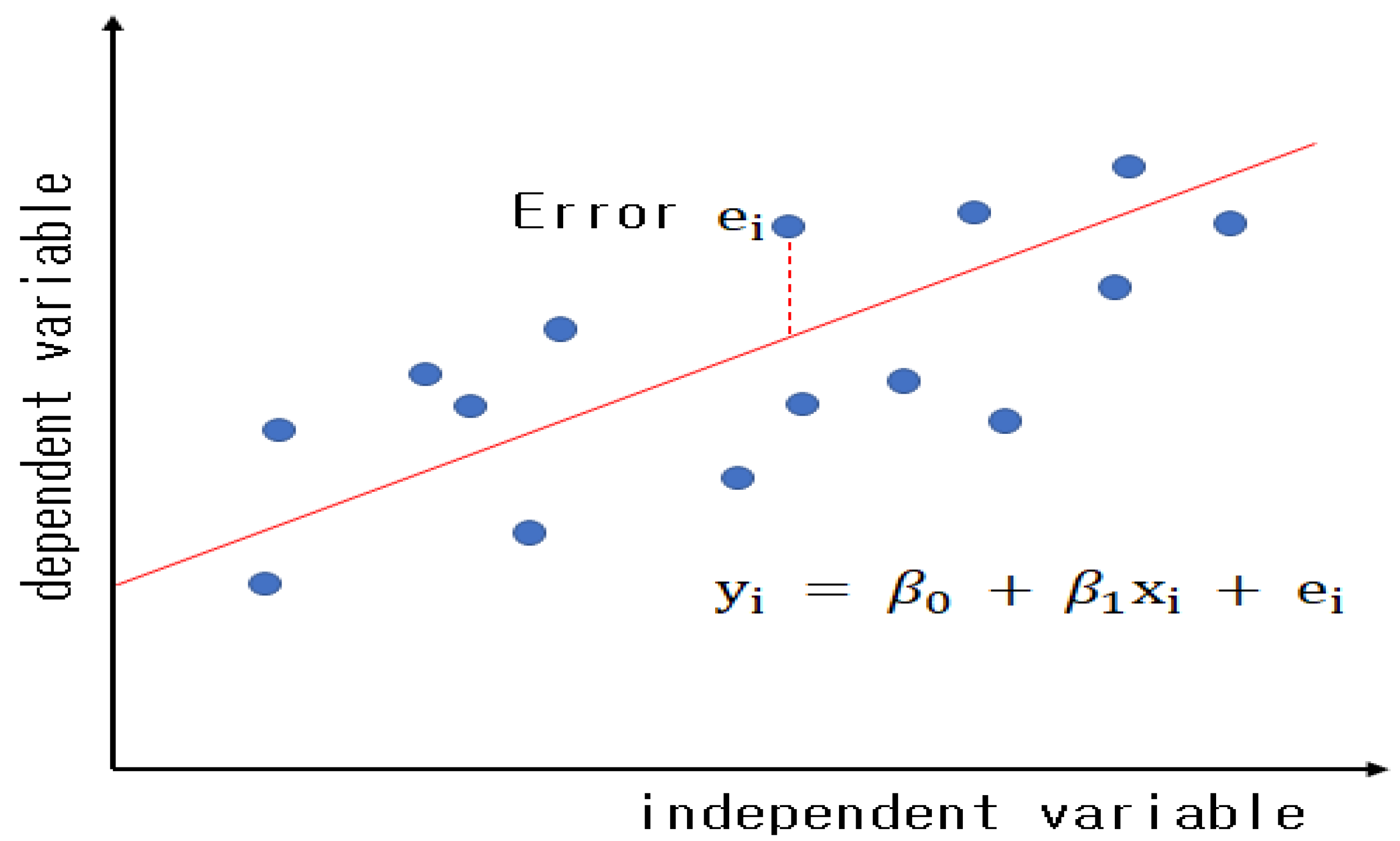
In the computing performed in general-used fuzzy inference systems, ANNs, and deep learning methods, the model output appears in a crisp form or as numbers. If the model output is in a crisp form or a number with a clear value, the numerical error relative to the actual output value can be calculated; however, difficulties occur when the difference between the model and actual output is expressed linguistically. However, in GrC, the model output is expressed in a soft form or as a fuzzy set; hence, GrC is effective at handling and processing data and information that are uncertain, incomplete, or with vague boundaries. In the actual world, people mainly use linguistic expressions rather than numerical expressions, and the brain, which makes inferences in uncertain and incomplete environments, utilizes linguistic values instead of numerical values to perform inferences and make decisions. Accordingly, GrC can represent the process by which humans think and make decisions. The following studies on GrC have been conducted [26,27,28,29]. Zhu [30] proposed a novel approach that develops and analyzes a granular input space and designed a granular model accordingly. Truong [31] proposed fuzzy possibilistic C-means (FPCM) clustering and a GrC method to solve anomalous value-detection problems. Zuo [32] proposed three types of granular fuzzy regression-domain adaptative methods, to apply GrC to transfer learning. Hu [33] proposed a method that adopts GrC to granularize fuzzy rule-based models and assess the proposed models. Zhao [34] made long-term predictions about energy systems in the steel industry by designing a granular model based on IGs created via fuzzy clustering. By analyzing the aforementioned research, it has become possible to create IGs that are generated via GrC, and to use these to design a granular model (GM), as well as calculate soft form output and express it linguistically. In addition, performance evaluation methods are proposed to evaluate the prediction performance of soft form output. However, studies are required to improve the prediction performance of granular models by creating optimal IGs, including methods for generating IGs and setting their form and size.

Conventional fuzzy clustering creates circle-shaped clusters starting at the cluster’s center in the input space. However, when the input space’s data exhibits geometric features, a problem emerges in which the clustering is not properly performed. To address this problem, Gustafuson-Kessel (GK) clustering is employed, as it can generate clusters while considering the geometric features of the data. This study proposes context-based GK (CGK) clustering, which considers both the input space and also the output space during existing GK clustering to generate geometrically-shaped clusters. This study also designed a CGK-based granular model that utilizes the proposed context-based GK clustering to generate context-shaped IGs in the output space and geometrically-shaped IGs in the input space. In addition, to resolve the problem of geometric increases in the numbers of rules when large amounts of data are adopted, this study proposes a CGK-based granular model with a hierarchical structure that combines the CKG-based granular model and the normal prediction model into an aggregate structure, such that meaningful rules can be generated. The remainder of this paper is organized as follows. Section 2 describes fuzzy clustering and GK clustering, while Section 3 describes IGs, existing granular models, the proposed context-based GK clustering, and the CGK-based granular model. Section 4 describes the hierarchical CGK-based granular model that is combined into an aggregate structure, and Section 5 verifies the validity of the proposed method by analyzing its performance using prediction-related benchmarking data. Finally, Section 6 presents this paper’s conclusions and future research plans.

2. Data Clustering

Clustering is the task of placing data sets into clusters, such that the data in the same cluster are more mutually similar than data in other clusters. It is mainly used in data search and analysis, and as a data analysis method, it is adopted in various fields such as image analysis, bioinformatics, pattern recognition, and machine learning. Because the concept of clustering cannot be precisely defined, various clustering algorithms exist. These include connectivity based clustering, centroid based clustering, distribution based clustering, density based clustering, and grid based clustering, while a typical clustering method is fuzzy clustering.

2.1. Fuzzy Clustering

Fuzzy clustering is a method that was developed by Dunn and improved by Bezdek [35], which exhibits the feature of allowing the given data to belong to two or more clusters. In non-fuzzy clustering, the given data can only belong to exactly one cluster; hence, it is divided into separate clusters. In fuzzy clustering, data can belong to two or more clusters according to the membership values. For example, a banana can be yellow or green (non-fuzzy clustering criteria, or it can be yellow and green (fuzzy clustering criteria). Here, certain parts of the entire banana can be yellow, and they can be green. The banana can belong to green (green = 1), and it can belong to yellow (yellow = 0.5) and green (green = 0.5), which is not yellow (yellow = 0). The membership values can be between zero and one, while the sum of the membership values is 1. Membership values are assigned to the given data. These membership values numerically indicate the extent to which the data belongs to each cluster. If the data has a low membership value, it can be known that it is on the edge of the cluster; conversely, if it has a high membership value, it can be deduced that it is in the center part of the cluster.

Fuzzy clustering can be generalized by the following formulas.

$$J_m={{\displaystyle \sum }}_{i=1}^N{{\displaystyle \sum }}_{k=1}^c{u}_{ki}^m{d}^2\left(x_i, v_k\right)$$

(1)

$${{\displaystyle \sum }}_{k=1}^c{u}_{ki}=1, \forall i \in \left\{1, 2, \dots , N\right\}$$

(2)

where $X=\left\{x_1, x_2,\dots , x_N\right\} \in R^{N\times D}$ and $x_i\in R^{1\times D}$ represents the data and data items, respectively. $N$ denotes the number of data items, and $c$ is the number of clusters, which is $2\le \mathrm{c}\le N$. $u_{ki} \in R$ represents the membership value of the kth $x_i$, and $m\in Z^{+}$ is the fuzzification coefficient for the fuzzy membership values.

The cluster center and fuzzy membership function are obtained via an iterative process by minimizing Equation (1) according to the constraint conditions defined in Equation (2). Therefore, the objective function is modified using Lagrange multipliers and expressed as:

$$J_m={{\displaystyle \sum }}_{i=1}^N({{\displaystyle \sum }}_{k=1}^c{u}_{ki}{}^m{d}^2\left(x_i,v_k\right)+{\lambda }_i\left(1-{{\displaystyle \sum }}_{k=1}^c{u}_{ki}\right))$$

(3)

where ${\lambda }_i$ denotes the Lagrange multiplier. Therefore, the clustering problem involves identifying the cluster center set $v^{*}= \left\{v_k{}^{*}, \forall k \in \left\{1, 2, \dots , c\right\}\right\}$ and the fuzzy membership function set $U^{*}= \left\{u_{ki}{}^{*}, \forall k \in \left\{1, 2, \dots , c\right\}, \forall i \in \left\{1, 2, \dots , N\right\}\right\}$ by minimizing Equation (3). The minimization of cluster centers $v_k{}^{*}$ can be obtained via Equation (4), and the minimization of the fuzzy membership functions can be obtained using Equation (5), which are expressed as:

$$v_k{}^{*}=\frac{{{\displaystyle \sum }}_{i=1}^N{u}_{ki}{}^m{x}_i}{{{\displaystyle \sum }}_{i=1}^N{u}_{ki}{}^m}$$

(4)

$$u_{ki}{}^{*}=\frac{1}{{{\displaystyle \sum }}_{j=1}^c{(\frac{d^2\left(x_i, v_k\right)}{d^2\left(x_i, v_j\right)})}^{\frac{1}{\left(m-1\right)}}}$$

(5)

Equations (4) and (5) are computed repeatedly to obtain the final cluster centers and fuzzy membership functions.

2.2. Fuzzy Clustering That Considers the Output Space

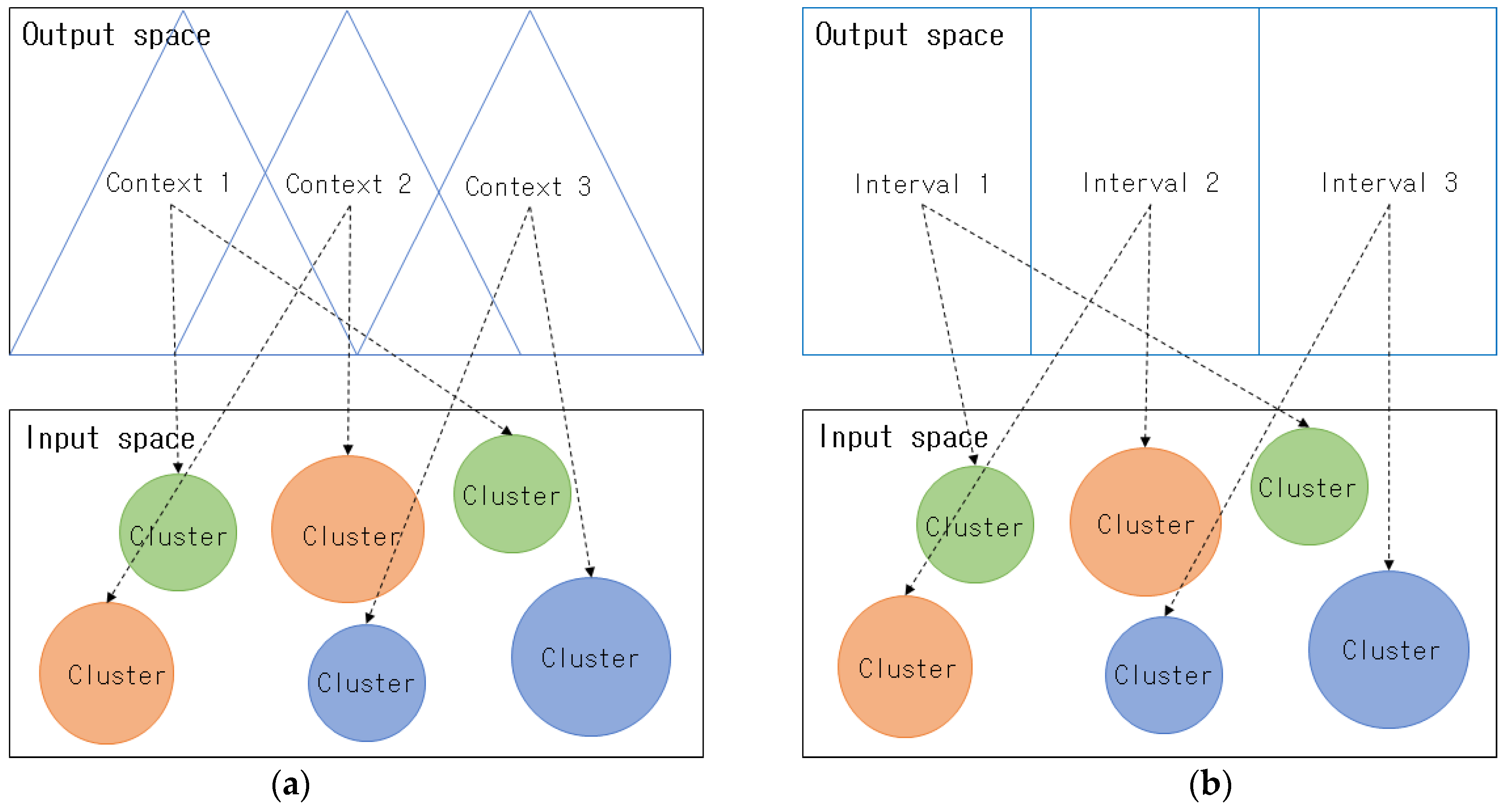
The aforementioned fuzzy clustering is a clustering that considers the features of the data in the input space. A fuzzy clustering that considers the output space generates clusters by considering both the features of the data in the input space and also the similarity and features of the data in the output space. This clustering type includes context-based fuzzy C-means (CFCM) clustering and interval-based fuzzy C-means (IFCM) clustering [36], which differ according to how the output space is divided. Figure 1. illustrates the fuzzy clustering that considers the output space. In Figure 1a. triangle-shaped contexts (fuzzy sets), which are IGs, are created in the output space, while clusters that correspond to each context are created in the input space. In Figure 1b interval-shaped IGs are created in the output space, and clusters that correspond to each interval are created in the input space.

In normal fuzzy clustering, clusters are created using only the Euclidean distance between the cluster centers and the data in the input space, without considering the features of the data in the output space. However, in context-based fuzzy clustering, triangle-shaped contexts (fuzzy sets) are created in the output space using the method proposed by Pedrycz [37,38], while clusters are created via fuzzy clustering in each context; hence, clusters can be created in a more sophisticated manner than in conventional fuzzy clustering. 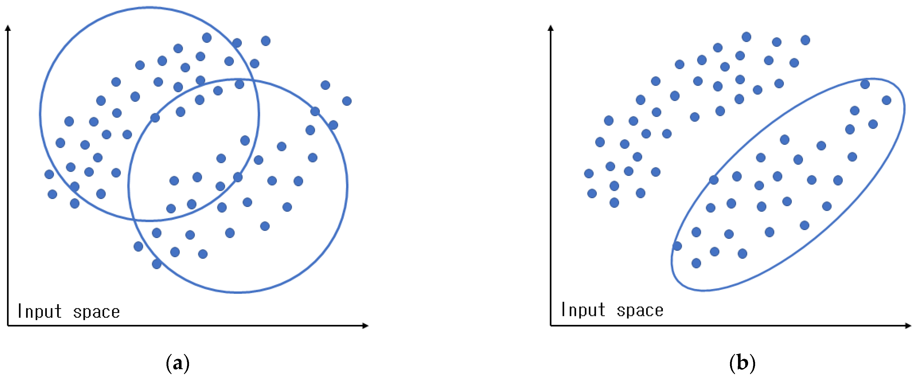Figure 2a presents normal fuzzy clustering, and Figure 2b shows clusters that were created in context-based fuzzy clustering by considering the features of the output space.

As illustrated in Figure 2, fuzzy clustering creates clusters using the distance between the cluster centers and the data in the input space without considering the properties of the data in the output space. In contrast, context-based fuzzy clustering creates clusters by considering the properties of the data in the output space; hence, it can create clusters more efficiently than conventional fuzzy clustering.

The context of the data in the output space can be expressed as $D:T \to \left[0, 1\right]$. D represents all of the data in the output space. Here, it is assumed that the context for the given data can be adopted. $f_k=T\left(d_k\right)$ represents the extent to which the kth data belongs in the context created in the output space. $f_k$ can be a value between zero and one, and the requirements for the membership matrix are as expressed in Equation (6) owing to the aforementioned properties.

$$U\left(f\right) =\{eqalign{u}_{ik}\in \left[0,1\right]\mid {{\displaystyle \sum }}_{i=1}^c{u}_{ik}=f_k \forall k \mathrm{and} 0<{{\displaystyle \sum }}_{k=1}^N{u}_{ik}<N\}$$

(6)

$$u_{ik}=\frac{f_k}{{{\displaystyle \sum }}_{j=1}^c{(\frac{\parallel x_k - c_i\parallel }{\parallel x_k - c_j\parallel })}^{\frac{2}{m-1}}}$$

(7)

The membership matrix $U$ updated by Equation (6) can be expressed as Equation (7). Here, m is the fuzzification coefficient, and $m=2$ is generally used. For the contexts, the output space is uniformly divided into fuzzy set forms, while the degree of membership $f_k$ is obtained. Usually, the output space is divided uniformly; however, it can be divided flexibly according to a Gaussian probability distribution according to the features of the data. The sequence in which the context-based fuzzy clustering is performed is presented below.

[Step 1] Select the number of contexts that can be expressed linguistically and the number of clusters that can be created in each context, and then initialize the membership matrix U with arbitrary values between zero and one. The numbers of the contexts and clusters can be set as the same number, or different values can be set by the user.

[Step 2] Divide the output space uniformly into fuzzy set forms and create fixed-sized contexts that can be expressed linguistically. In addition, a Gaussian probability distribution can be used to flexibly divide the output space and create contexts of different sizes.

[Step 3] Use Equation (8) to calculate the centers of the clusters in each context.

$$c_i=\frac{{{\displaystyle \sum }}_{k=1}^N{u}_{ik}{}^m{x}_k}{{{\displaystyle \sum }}_{k=1}^N{u}_{ik}{}^m}$$

(8)

[Step 4] Use Equations (9) and (10) to calculate the objective function. Here, the calculated value is compared to the previous objective function value, and the above process is repeated, provided it is greater than the threshold value that was set, or the process ends if it is less than the threshold value.

$$J={{\displaystyle \sum }}_{i=1}^c{{\displaystyle \sum }}_{k=1}^N{u}_{ik}{}^m{d}_{ik}{}^2$$

(9)

$$\left|J^h-J^{h-1}\right| \le \varepsilon$$

(10)

where $d_{ik}$ denotes the Euclidean distance between the kth data and $i$th cluster center, and h repress nets the number of iterations.

[Step 5] Equation (7) is adopted to update the membership function U, and Step 3 is performed.

2.3. GK Clustering

Regardless of the data in the input space belonging to a cluster, the cluster is normally determined by the distance between the data and the center of each cluster. As described in Section 1, fuzzy clustering adopts Euclidean distance to create clusters. Euclidean distance is primarily used when circle-shaped clusters are created, and it has the problem of being unable to create clusters that are not circle-shaped. To resolve this problem, GK clustering was proposed [39,40,41], as it can create geometrically-shaped clusters. GK clustering employs Mahalanobis distance, rather than Euclidean distance, to calculate the distance between cluster centers and data. Figure 3 illustrates clusters that were created in fuzzy and GK clustering, and Equation (11) presents the Mahalanobis distance.

$$d_{GK}{}^2\left(x_k, v_i\right) = \parallel x_k-v_i{\parallel }_{A_i}{}^2={(x_k-v_i)}^T{A}_i\left(x_k-v_i\right)$$

(11)

where $d_{GK}{}^2$ denotes the square of the distance between the ith cluster’s center $v_i$ and the kth data $x_k$, while $A_i$ is the variance matrix of the ith cluster. In GK clustering, Equation (12) is used to calculate the variance matrix $A_i$ in Equation (11).

$$A_i=\frac{{{\displaystyle \sum }}_{k=1}^N{u}_{ik}{}^m\left(x_k-v_i\right){(x_k-v_i)}^T}{{{\displaystyle \sum }}_{k=1}^N{u}_{ik}{}^m}$$

(12)

The variance matrix that is calculated using Equation (12) is adopted when calculating the distance between the cluster center and the data in Equation (13):

$$D_{GK}{}^2={(x_k-v_i)}^T[{\rho }_i det(A_i{)}^{\frac{1}{N}}{A}_i{}^{-1}]\left(x_k-v_i\right)$$

(13)

where ${\rho }_i$ denotes the volume of each cluster. When $A_i$ is calculated in Equation (13), the matrix may become zero if the number of data is insufficient; hence, the minimum value is limited using Equation (14).

$$\left(1-\gamma \right)A_i+\gamma det{(A_i)}^{\frac{1}{N}}I\to A_i$$

(14)

where $A_i$ is the variance matrix that is calculated using all data, while I and $\gamma$ denote the unit matrix and weight value constant, respectively. The eigen value and eigen vector can be calculated from the variance matrix. The calculated maximum eigen value is used to limit the minimum eigen value, such that the shape of the cluster can be maintained geometrically.

3. IG Creation and Granular Model Design

3.1. Creating Rational IG

Computing and inferences in GrC are centered on IGs, which are considered fundamental concepts and algorithms, rather than being centered on numbers. IGs are a core element in GrC because they play an important role in knowledge representation and processing [42,43,44]. Although IGs created using various types of clustering are relatively limited, they can reflect the general structure of some original data. Original data comprising numbers cannot depict the features and connections in the data, but IGs make this possible. Rational IG creation is focused on using the original data to create meaningful IGs. To create rational IGs, two requirements must be satisfied: coverage and specificity. 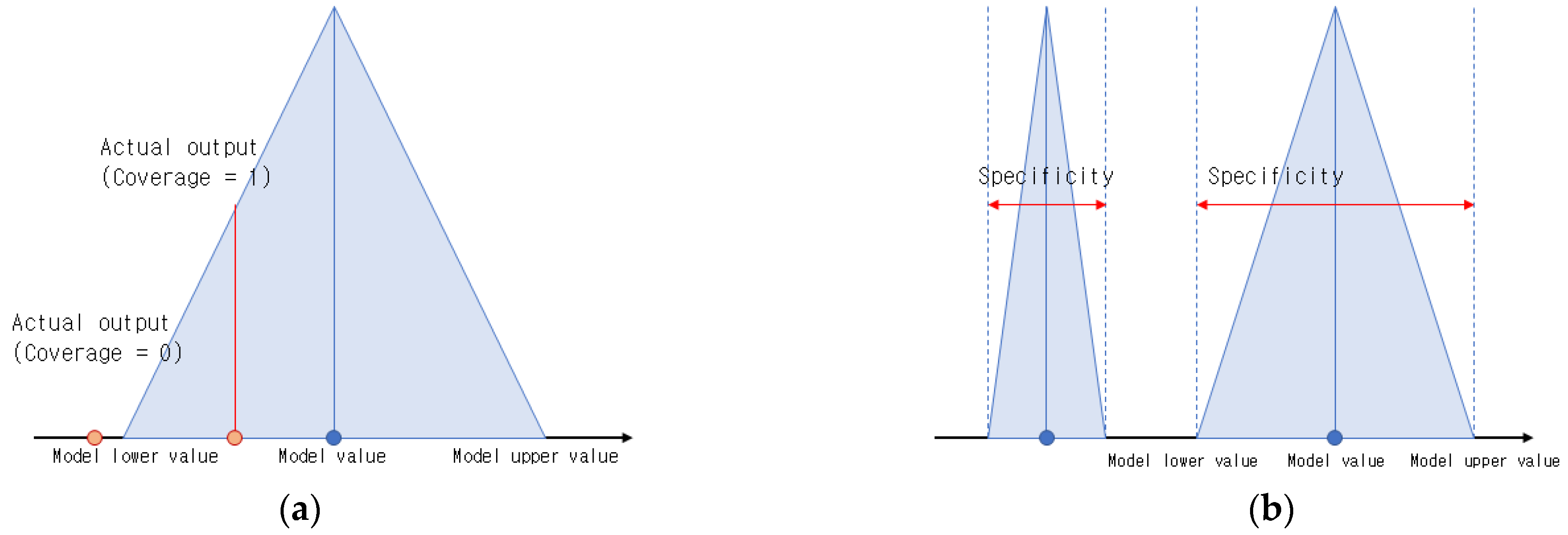Figure 4. Presents the coverage and specificity in IGs.

Coverage refers to whether the target data is included in the formed IG. In other words, it shows how much of the overall target data has accumulated within the IG’s range, including the extent of the accumulation. The more data that accumulates in the IG, the higher the coverage value. This can verify the validity of the IG, and the model may be better in terms of modeling functions. incl, which is the degree of inclusion and is specified according to the form in which the IG $Y_k$ is created. When $Y_k$ is in context form, incl has a value close to one when $y_k$ is included in $Y_k= \left[y_k{}^{-}, y_k{}^{+}\right]$, and it has a value close to zero when it is not included. In other words, coverage can be adopted to count the number that includes the data $y_k$ in the granularized output of the granular model, while an average value can be calculated for all data. Ideally, the coverage has a value that is close to one, and all data is included in the granular model’s output.

$$Coverage=\frac{1}{N}{{\displaystyle \sum }}_{k=1}^{N}incl \left(y_k, Y_k\right)$$

(15)

Specificity represents how specifically and semantically the IG $Y_k$ can be described. In general, the specificity of a given IG $Y_k$ must satisfy Equation (16). In other words, the IG must be created with as much detail as possible, and each IG must have a meaning that can be described. When an IG is in context form, the specificity becomes higher as the interval, i.e., the distance between the upper and lower bounds, becomes narrower. If the IG $Y_k$ is reduced to point form, the specificity arrives at a value close to one.

$$\mathrm{if} Y_k\subset Y_k{}^{\prime } \mathrm{then} specificity\left(Y_k\right) \succ specificity\left(Y_k{}^{\prime }\right), \mathrm{and} specificity\left(\left\{y\right\}\right) =1$$

(16)

$$Specificity=\frac{1}{N}{{\displaystyle \sum }}_{k=1}^{N}exp\left(-\left|y_k{}^{+}-y_k{}^{-}\right|\right)$$

(17)

A continuous decreasing function of the interval length can be considered instead of the exponential function used in Equation (17). Coverage and specificity can be adopted to evaluate the IG’s validity and the granular model’s prediction performance. In other words, the granular model can be evaluated by considering the coverage and specificity of the IG, and a method that can simultaneously maximize coverage and specificity should be determined. These two properties have a trade-off relationship. This implies that the higher the coverage value, the lower the specificity value. Rational IGs can be represented by Equation (18), and this is called the PI.

The PI plays an important role in evaluating the model’s accuracy and clarity, and various methods for evaluating model performance have been developed. General performance evaluation methods include root-mean-square error (RMSE) and mean absolute percentage error (MAPE). RMSE evaluates performance by subtracting the model’s predicted values from the actual predicted values, calculating the mean of the squares, and squaring the obtained value. MAPE evaluates performance by subtracting the model’s predicted value from the actual output value and dividing by the model’s predicted value. These performance evaluation methods are mainly used when the model’s output value is a numerical value. However, in the case of granular models comprise IGs, the model output is not a numerical value but an IG; hence, it is difficult to evaluate the model using general performance evaluation methods. To address this issue, studies are actively being conducted on adopting coverage and specificity as performance evaluation methods for granular models [45,46,47,48,49]. The higher the PI, the more meaningful the IG, and granular models with excellent performance can be designed.

$$\mathit{Performance} \mathit{index}=coverage\left(\varepsilon \right) · specificity\left(\varepsilon \right)$$

(18)

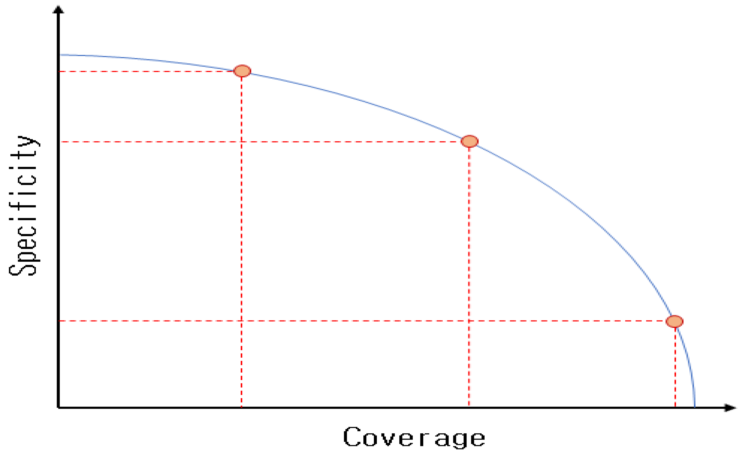
The PI value obtained from a granular model can be adopted to represent the relationship between coverage and specificity as coordinates, and the changes in model performance, which are related to changes in the PI value, can be observed. Figure 5 illustrates the trade-off relationship between coverage and specificity. If coverage approaches zero, specificity approaches one, and the shape of the IG approaches a point. It can be observed that as the coverage increases, the size of the IG increases, but the specificity decreases.

3.2. Fuzzy-Based Granular Model

Because the inference values of fuzzy rule-based inference systems used in various real-world fields of application are numeric values, there are limitations to describing these results linguistically. Fuzzy granular models, which are designed based on IGs that are created using fuzzy clustering, can express and process knowledge because their output values are IGs. Fuzzy granular models are created by granularizing a predetermined level of information in the data included in A. Owing to the granular properties of the data, granularized output is created from the variables of an existing fuzzy model with numerical input and output. This is based on the rational IG creation method described in Section 3.2. The IGs used in the fuzzy granular model exhibit the shapes of the fuzzy sets. The IG’s level of granularization is assumed to be $\varepsilon \left(\varepsilon \in \left[0, 1\right]\right)$. The granularization level creates the IG $a_{i0}$ with a fuzzy set shape by allowing IGs of the given level $\varepsilon \left(\varepsilon \in \left[0, 1\right]\right)$, which can be described as shown below, due to $a_{i0}, a_{i1}, a_{i2}, \dots , a_{iN}$, which represent the data in each rule’s output space.

$$G\left(a_{i0}\right) = \left[min\left(a_{i0}\left(1 - \varepsilon \right), a_{i0}\left(1 + \varepsilon \right)\right), max\left(a_{i0}\left(1 - \varepsilon \right), a_{i0}\left(1 + \varepsilon \right)\right)\left] = \right[a_{i0}{}^{+}, a_{i0}{}^{-}\right] = A_{i0}$$

(19)

Using the same method, the IGs $A_{i1}, A_{i2}, \dots , A_{iN}$ are created by granularizing $a_{i1}, a_{i2}, \dots , a_{iN}$, which represent the data in the output space. A general fuzzy granular model divides the output space uniformly to create triangle-shaped contexts and clusters in each context. The fuzzy granular model’s output value $Y$ is expressed in context form, and each fuzzy rule regarding the input $x_k$ creates the following IG output:

$$\mathrm{if} x_k\in {\Omega }_i, \mathrm{then}{Y}_{ik}=f_i\left(x_k,A_i\right) =A_{i0}\oplus A_{i1}\otimes x_{k1}\oplus A_{i2}\otimes x_{k2}\oplus \dots \oplus A_{iN}\otimes x_{kN}$$

(20)

The following method is used to calculate $Y_k$, which is the IG output in context form that was created based on all fuzzy rules.

$$Y_k={{\displaystyle \sum }}_{i=1}^c{\Omega }_i\left(x_k\right) \oplus Y_k$$

(21)

where ⊕, ⊗ represent the completed addition and multiplication operations for each IG, respectively. Figure 6. Presents the structure of the fuzzy granular model.

3.3. CGK Clustering

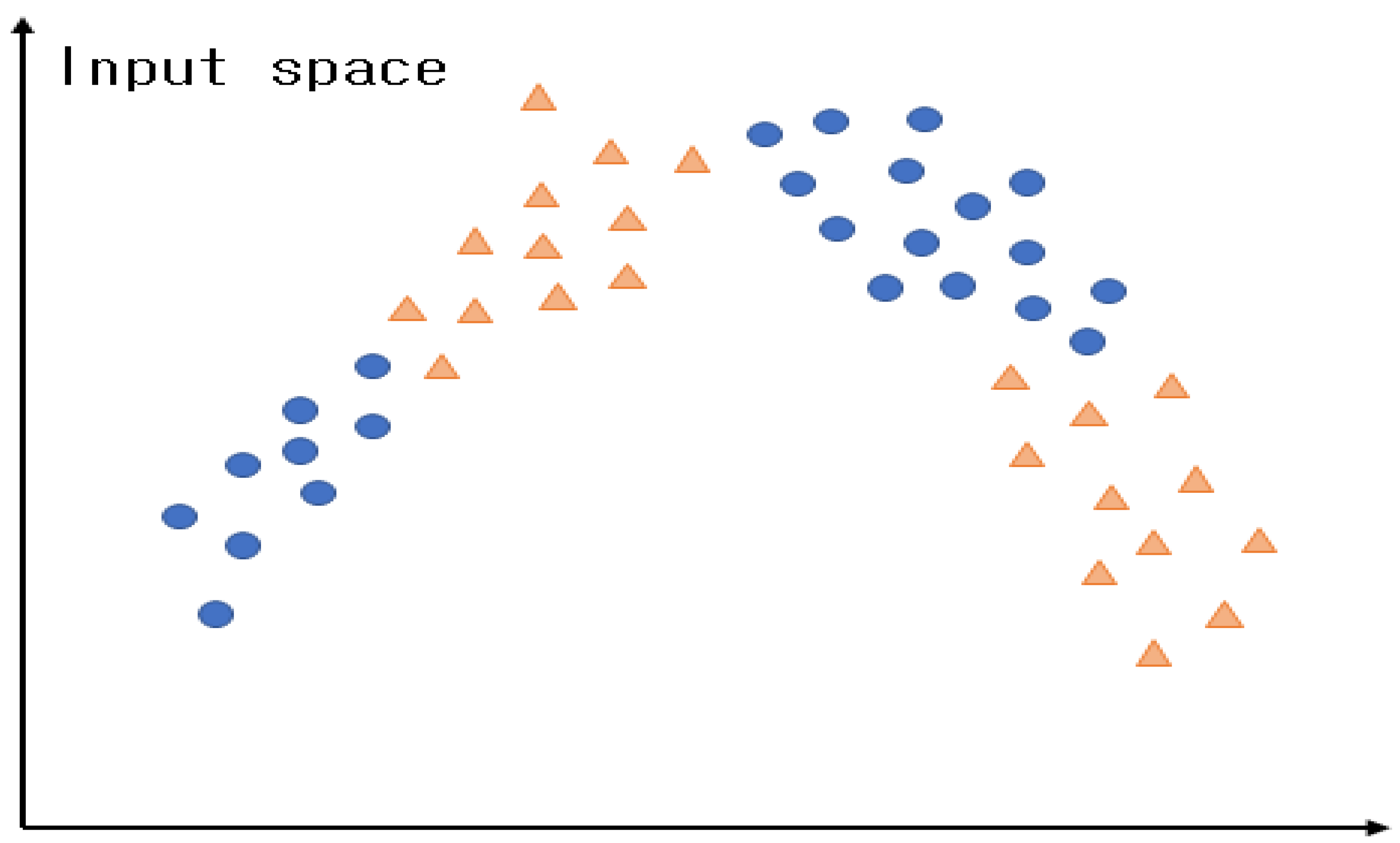
CGK clustering is a clustering method that considers the output space. It creates clusters based on the correlations between the data in the input and output spaces by considering the output space in conventional GK clustering. It is assumed that there are data with two features. The data above can be depicted in red and blue according to the dependent variable. Figure 7. Presents the data with two features.

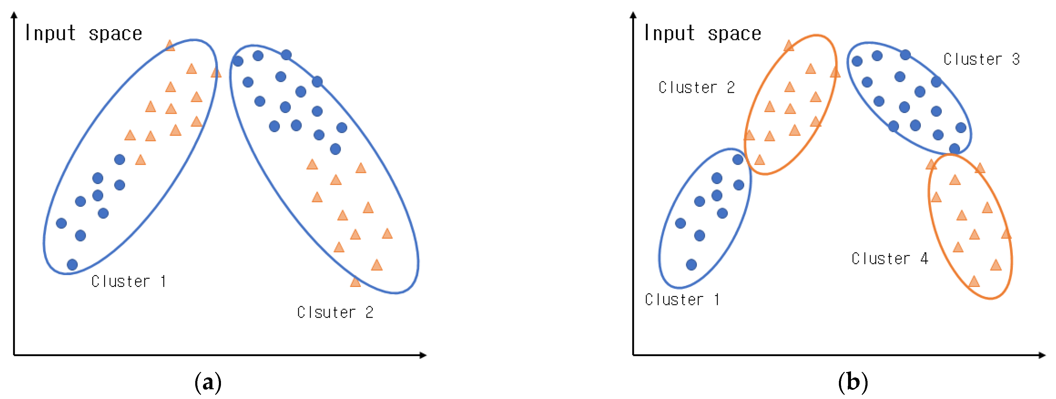
Figure 8a presents clusters created via normal GK clustering. In Figure 8a, it can be observed that the features of the data in the input space were considered when creating the clusters; however, the features of the output space were not considered. Figure 8b presents clusters created via CGK clustering that consider the output space. As illustrated in this figure, clusters are created by considering both the input and output spaces; hence, the features of the data in the output space can be preserved, and more efficient clusters can be created than in normal GK clustering. 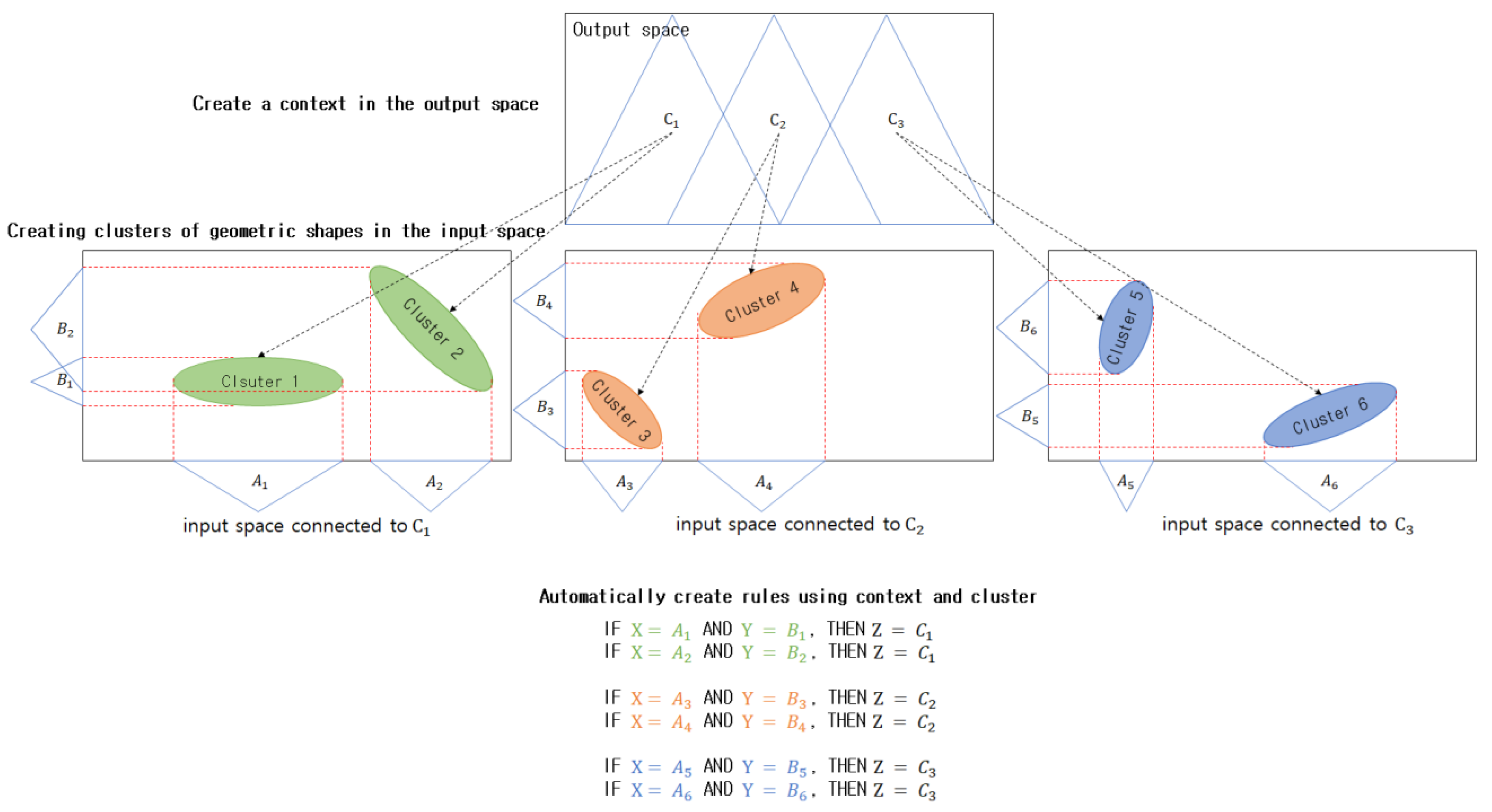Figure 9. Illustrates the concept of CGK that considers the output space.

The context regarding the data in the output space can be expressed as expressed in Equation (22). Here, D denotes the data in the output space. If it is assumed that a context-shaped IG is adopted for the given data in the output space, $f_k=T\left(d_k\right)$ represents the degree to which the context created in the output space belongs to the kth data.

$$D:T \to \left[0, 1\right]$$

(22)

Fuzzy clustering adopts Euclidean distance to create clusters, while GK clustering improves upon this by creating clusters with Mahalanobis distance using Equation (11).

Where $A_i$ is a matrix with $det\left(A_i\right) ={\rho }_i$, which is a fixed constant for each i. Because fuzzy clustering uses Euclidean distance, it exhibits excellent performance for only problems that create circle-shaped clusters. To circumvent this disadvantage, GK clustering adopts $d_{GK}{}^2\left(x_k, v_i\right)$ to extend the Euclidean distance of fuzzy clustering, such that clusters with various geometric shapes can be created, and it allows the distance standard to adapt to local areas. The objective functions are expressed in Equations (23)–(25).

$$J_m{}^{GK}\left(\mu , v\right) ={{\displaystyle \sum }}_{k=1}^n{{\displaystyle \sum }}_{i=1}^c{\mu }_{ik}{}^m{d}_{GK}{}^2\left(x_k, v_i\right)$$

(23)

$$v_i=\frac{{{\displaystyle \sum }}_{k=1}^n{\mu }_{ik}{}^m{x}_k}{{{\displaystyle \sum }}_{k=1}^n{\mu }_{ik}{}^m}$$

(24)

$${\mu }_{ik}=\frac{\parallel x_k-v_i{\parallel }_{A_i}{}^{\frac{-2}{\left(m-1\right)}}}{{{\displaystyle \sum }}_{j=1}^c\parallel x_k-v_j{\parallel }_{A_j}{}^{\frac{-2}{\left(m-1\right)}}}$$

(25)

Equations (23)–(25) are repeated in each context generated in the output space to create geometrically-shaped clusters. Below is the sequence in which context-based GK clustering is performed.

[Step 1] The number of contexts that can be expressed linguistically and the number of clusters that are created in each context are selected, as well as ɛ. Here, ɛ sets the degree of the geometric shape, and a value greater than zero must be selected. The membership function U is initialized with values between zero and one. The numbers of contexts and clusters can be set to be the same, or they can be set differently.

[Step 2] Context-shaped IGs with fixed sizes can be created by uniformly dividing the output space, while context-shaped IGs with different sizes can be created by via a Gaussian probability distribution.

[Step 3] Equation (24) is adopted to calculate the centers of the clusters in the contexts in the output space and a membership matrix.

[Step 4] Equations (23) and (26) are adopted to calculate an objective function, and the aforementioned process is repeated if the calculated value is greater than the previous objective-function value. Conversely, if the calculated value is less than the previous objective-function value, the above process ends.

$$\parallel {\mu }^t-{\mu }^{t-1}\parallel \le \varepsilon$$

(26)

3.4. CGK-Based Granular Model Design

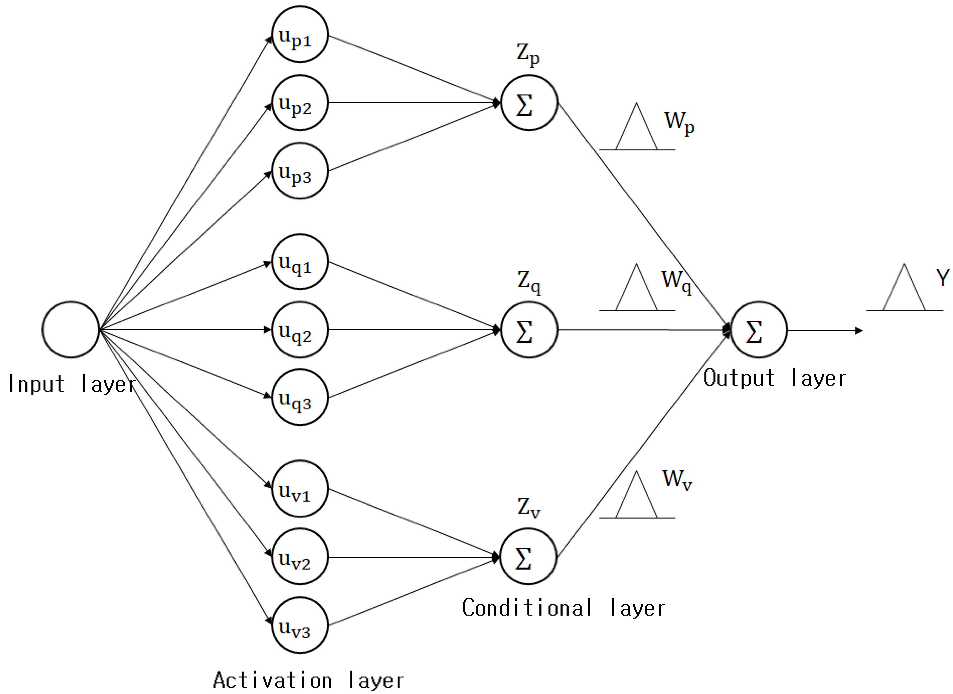
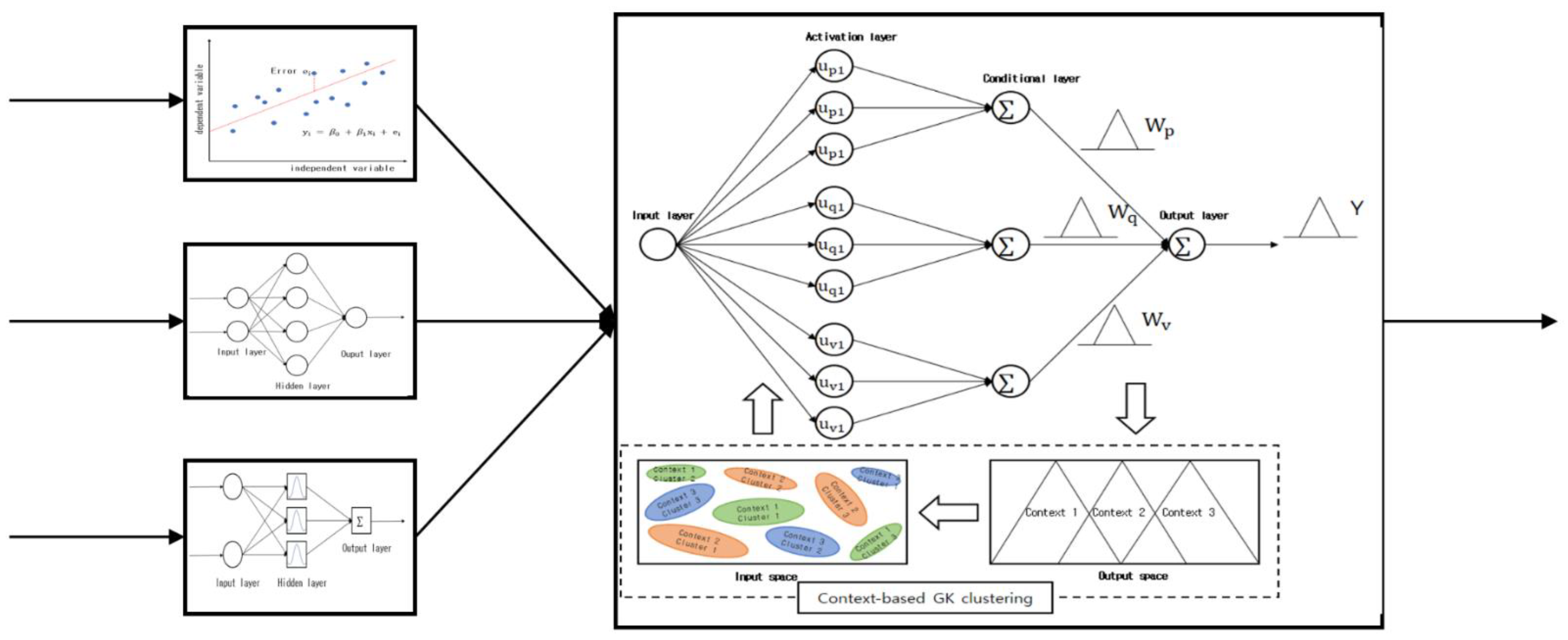
GK granular models are designed to adopt CGK clustering that considers the output space, to create context-shaped IGs in the output space and create geometrically-shaped clusters in each context. Figure 10. presents the structure of a GK granular model in which three contexts are created in the output space and three clusters are created in each context. As illustrated in the figure, there are conditional and conclusion variables. The conclusion variables represent the context-shaped IGs that are created in the output space, while the conditional variables represent the centers of the clusters that are created in each context, i.e., IGs that are created in the input space. As mentioned above, a uniform creation method and a flexible creation method can be adopted to create the contexts in the output space. The GK granular model’s final output value Y is calculated using Equation (27).

$$Y={{\displaystyle \sum }}_{\oplus }^{}{W}_t\otimes z_t$$

(27)

Here, the addition and multiplication symbols ⊕, ⊗ represent the completed addition and multiplication operations for the IGs, respectively. Fuzzy sets are created during the process of handling the GK granular model conditions. At this point, the clusters created via CGK clustering can be represented by the GK granular model’s hidden layer. The area between the hidden and output layers is expressed as a context that can be described linguistically. The sum, which is the GK granular model’s final output, can be expressed using all contexts as expressed in Equation (28):

$$Y=\left(z_{11}\otimes A_1\oplus z_{12}\otimes A_1\oplus \dots \oplus z_{1n1}\otimes A_1\right) \oplus \left(z_{21}\otimes A_2\oplus z_{22}\otimes A_2\oplus \dots \oplus z_{2n2}\otimes A_2\right) \oplus \dots \left(z_{c1}\otimes A_c\oplus z_{c2}\otimes A_c\oplus \dots \oplus z_{cnc}\otimes Ac\right)$$

(28)

The GK granular model’s final output is expressed as a triangle-shaped context, and it can be expressed as a fuzzy set:

$$Y_i= \left(y_i{}^{-}, y_i, y_i{}^{+}\right)$$

(29)

where $y_i{}^{-}, y_i, \mathrm{and} y_i{}^{+}$ denote the GK granular model’s lower bound, model, and upper bound values, respectively, and they refer to each of the triangle-shaped context’s points. The lower bound, model, and upper bound values can be expressed by Equations (30)–(32):

$$y_i{}^{-}= \left(z_{11}{a}_1+z_{12}{a}_1{}^{-}+\dots +z_{1n1}{a}_1{}^{-}\right) +\dots \left(z_{c1}{a}_c{}^{-}+z_{c2}{a}_c{}^{-}+\dots +z_{cnc}{a}_c{}^{-}\right)$$

(30)

$$y_i= \left(z_{11}{a}_1+z_{12}{a}_1+\dots +z_{1n1}{a}_1\right) +\dots \left(z_{c1}{a}_c+z_{c2}{a}_c+\dots +z_{cnc}{a}_c\right)$$

(31)

$$y_i{}^{+}= \left(z_{11}{a}_1+z_{12}{a}_1{}^{+}+\dots +z_{1n1}{a}_1{}^{+}\right) +\dots \left(z_{c1}{a}_c{}^{+}+z_{c2}{a}_c{}^{+}+\dots +z_{cnc}{a}_c{}^{+}\right)$$

(32)

When CGK clustering is performed, the membership matrix $U$ can be expressed as values between zero and 1, while the membership matrix’s requirements can be expressed as:

$$U\left(f\right)=\{eqalign{u}_{ik}\in \left[0, 1\right]\mid {{\displaystyle \sum }}_{i=1}^c{u}_{ik}=f_k \forall k \mathrm{and} 0<{{\displaystyle \sum }}_{k=1}^N{u}_{ik}<N\}$$

(33)

Here, the contexts are created by uniformly or flexibly dividing the output space into fuzzy set shapes. The GK granular model’s structure is as follows. In the input layer, data is received and enters the GK granular model. The activation layer is the cluster activation step in which clusters that correspond to the contexts that were created in the output space are created in the input space. The conditional layer performs conditional clustering in each context. The activation and conditional layers are connected, and the data information is adopted in GK clustering when a context is provided. The GK granular model is focused on the activation and conditional layers. The contexts are connected to the GK clustering in the conditional layer, and fuzzy sets are created by considering the features of the data in the input space. A specified number of clusters is created in each context, and the total number of nodes in the output layer is the same as the number of contexts. The final output values that are added up in the output layer are represented as a triangle-shaped context.

4. Granular Model Design with a Hierarchical Structure

4.1. CGK-Based Granular Model Design with a Hierarchical Structure

As the number of input variables for a fuzzy system and granular model increase, the number of rules increase geometrically. Large rule bases have the problem of reducing the computation efficiency of fuzzy systems and granular models. In addition, they make it difficult to understand the action of granular models, and complicate the adjustment of rules and membership functions. The possibility of generalizing fuzzy systems and granular models with large rule bases is minimized because various prediction-related fields of application provide limited amounts of data. To resolve these problems, rather than using a single fuzzy system and a single granular model, it is possible to design a granular model with a hierarchical structure in which these are mutually connected. Because the granular model is arranged in a hierarchical tree structure, the tree is called the hierarchical structure. The output of the low-level granular models in the hierarchical structure is adopted as the input for the high-level granular models. Granular models with hierarchical structures are computationally more efficient than single granular models with the same number of inputs, and are also designed with a simple structure [50,51,52].

Hierarchical structures that can be used in various prediction-related fields of application include incremental, aggregated, and cascaded structures. Figure 11. Presents each type of hierarchical structure. In incremental structures, input variables are combined in several stages, while output values are calculated at several levels. As illustrated in Figure 11, the granular model $G{M}_i{}^n$ is built with a 3-stage structure. Here, $i$ is the nth level’s granular model. In an incremental granular model, when $i$ is one, it means that there is one fuzzy inference system on each level. The nth level’s $i$th granular model’s jth input is called $x_{ij}{}^n$, while the nth level’s ith granular model’s kth output is called $y_{ik}{}^n$. When the input variables on each of the levels of an incremental granular model are selected, their ranks are determined according to their degrees of contribution to the final output value. The input variable with the highest degree of contribution is usually used on the lowest level; conversely, the input variable with the lowest degree of contribution is adopted on the highest level. In other words, low-rank input values depend on high-rank input values.

In an aggregate structure, the original data’s input variables are used on the lowest level, and the output of the low-level granular model that receives each input variable as the input is inputted in the high-level granular models, and the obtained results are combined. For example, the granular model $G{M}_{i_n}{}^n$ is built with two stages as, illustrated in Figure 11. $i_n$ is the index of the granular model on the nth level. The input variables in aggregated granular models are grouped for performing specific decision making. For example, an autonomous robot’s search task combines two tasks: searching while avoiding collisions with obstacles, and arriving at the goal. To perform the search task, the granular model adopts input variables related to obstacles. To perform the task of arriving at the goal, input variables related to the robot’s current position and movement direction are employed. Aggregated granular models can be modified to design parallel aggregated granular models that directly add up the outputs of low-level granular models to calculate their final output.

A cascaded structure is a structure that combines the aforementioned incremental structure with the hierarchical structure, and it is suitable for systems that include both correlated input variables and non-correlated input variables. It has a form in which the correlated input variables are grouped into an aggregated structure and the non-correlated input variables are added as an incremental structure.

4.2. CGK-Based Granular Model Design with an Aggregated Structure

This paper presents a design for a granular model that adopts an aggregated structure. When an aggregated structure is built, rather than using low-level and high-level granular models, the low level comprises LR (LR) models, neural network models, and radial basis function networks, and each prediction model’s output is adopts as the input for the high-level fuzzy granular model to calculate the final output.

An LR model [53] models the linear correlations between input and output variables. Figure 12 shows the concept of linear regression. Simple linear regression models are based on explanatory variables, while multiple linear regression models are based on two or more explanatory variables. Linear regression models estimate unknown parameters in the data. A linear regression model can be expressed as:

$$y_i = {\beta }_1{x}_{i1} + \dots + {\beta }_p{x}_{ip} + {\varepsilon }_i = x_i{}^T\beta + {\varepsilon }_i, i = 1, 2, \dots , n$$

(34)

where ${\beta }_i$ and p denote each independent variable’s coefficient and the number of parameters estimated by the linear regression model, respectively. $T$ indicates transposition, while $x_i{}^T\beta$ represents the inner product of $x_i$ and $\beta$. Furthermore, ${\varepsilon }_i$ is the error term, and it represents the error variables. This refers to the error between the dependent and independent variables.

Neural networks [54] are algorithms that are created with inspiration from biological neural networks in cognitive science and machine learning. These models can solve problems by altering the strength of the connections between synapses via the learning performed by the nodes that constitute the neural network by combining synapses. Figure 13. Presents the structure of a simple neural network. A simple neural network consists of an input layer, hidden layer, and output layer. The input layer inputs the data’s input variables into the neural network, and the number of input variables must equal the number of input layer nodes. Usually, no calculation is performed in the input layer, and the layer simply performs the role of passing the values on. The hidden layer is between the input and output layers. If there are two or more hidden layers, it is called a multi-layer neural network. The output layer calculates the neural network’s output. To achieve this, it adopts an activation function that is suitable for the problem to be solved.

A radial basis function network [55,56] is a neural network that adopts a radial basis function, instead of a sigmoid function, as the activation function in a conventional neural network structure. Figure 14. Presents the structure of a radial basis function network. A radial basis function network has a simple structure because there is only one hidden layer and the form of the output is linear; therefore, weight value calculations can be performed efficiently.

The outputs from a linear regression model, neural network, and radial basis function network are combined and adopted as the input of a high-level fuzzy granular model. The high-level fuzzy granular model determines the number of contexts created in the output space and the number of clusters created in the input spaces, and then creates the IGs. Accordingly, the final output of the hierarchical structure is calculated. Existing fuzzy granular models are limited in creating meaningful IGs in the input and output spaces when processing large-scale data, and they have the problem of long computation times. In contrast, the fuzzy granular model with a hierarchical structure proposed in this study has the advantages of being able to create meaningful IGs from large-scale data and reduce processing times by taking the data created by combining the output from the low-level linear regression model, neural network, and radial basis function network, as well as adopting it as the input of the high-level fuzzy granular model. Here, if the clustering used by the granular model is context-based fuzzy clustering, the model is a fuzzy granular model with a hierarchical structure, and if the clustering is context-based GK clustering, the model is a GK granular model with a hierarchical structure. Figure 15. Presents the structure of a granular model with a hierarchical structure.

5. Experiment and Results Analysis

To examine the validity of the CGK-based Granular Model (CGK-GM), which is the method proposed in this study, as well as the CGK granular model with an aggregated structure (AGM), the experiments were performed through a concrete compressive strength database [57] which are benchmarking databases used in the field of forecasting. For convenience in the experiments and the results analysis, the two proposed granular models are labeled CGK-GM, AGM. The databases used in the experiments are presented as follows. The concrete compressive strength database was collected by Tsinghua University in Taiwan, and it comprises 1030 instances and 9 variables. The input variables include the cement, fly ash, blast furnace slag, water, superplasticizer, coarse aggregate, fine aggregate, and time. The output variable is the concrete’s compressive strength.

Experimental Method and Results

In this study, the prediction performance of the granular model was evaluated by the Performance Index (PI) method, which is a performance evaluation method that is suitable for IGs and granular models, rather than the generally used evaluation methods. As expressed in Equation (18). The experiment method is presented as follows. Each database was divided into 50% learning data and 50% validation data, normalized to values between zero and one and then used in the experiments. The numbers of contexts (P) and clusters (C) in conventional GM, the proposed CGK-GM, and AGM were increased from 2 to 6 in increments of 1 during the experiments, while the fuzzification coefficient was fixed at 2. In addition, the experiments were performed using the uniform and flexible method of creating contexts.

The following shows the results of the concrete compressive strength prediction experiment.

Table 1. Performance index of GM that created context evenly.

	C	2	3	4	5	6
P
2		0	0	0	0	0
3		0	0	0	0	0
4		0.3165	0.3175	0.3191	0.3184	0.3191
5		0.4039	0.4184	0.4223	0.4175	0.4204
6		0.4031	0.4136	0.4183	0.4159	0.4276

shows the prediction performance of the existing GM that created the context uniformly, and

Table 2. Performance index of GM that created context flexibly.

	C	2	3	4	5	6
P
2		0	0	0	0	0
3		0.0097	0.0093	0.0097	0.0093	0.0090
4		0.2931	0.2947	0.2953	0.2945	0.2948
5		0.3897	0.3962	0.3962	0.3946	0.3960
6		0.4022	0.4120	0.4183	0.4212	0.4230

shows the prediction performance of the GM that created the context flexibly. Figure 16 shows the output value and actual output value of the existing GM, and Figure 17 shows the performance index value of the existing GM for the verification data. In Figure 16, the x-axis represents the number of verification data for the concrete compressive strength, and the y-axis represents the concrete compressive strength value. The black solid line is the actual concrete compressive strength value, and the red dotted line shows the output value of the existing GM. As shown in the figure, it can be confirmed that the GM output value predicts a large change in the actual output value, but does not predict a small change. In Figure 17, the x-axis represents the number of clusters created in the input space, and the y-axis represents the number of contexts created in the output space. The z-axis shows the performance index values for the verification data. As shown in the figure, it can be seen that when the number of contexts is 6 and the number of clusters is 6 when the contexts are created equally, the performance index value is 0.4276, which is the best.

Table 3. Performance index of CGK-GM that created context evenly.

	C	2	3	4	5	6
P
2		0	0	0	0	0
3		0.0204	0.0204	0.0204	0.0205	0.0206
4		0.3328	0.3315	0.3308	0.3295	0.3315
5		0.4409	0.4379	0.4350	0.4350	0.4300
6		0.4618	0.4629	0.4700	0.4618	0.4606

lists the prediction performance of the CGK-GM in which the contexts are uniformly generated, and

Table 4. Performance index of CGK-GM that created context flexibly.

	C	2	3	4	5	6
P
2		0	0	0	0	0
3		0.0295	0.0241	0.0282	0.0259	0.0233
4		0.3060	0.3070	0.3084	0.3070	0.3052
5		0.4182	0.4254	0.4183	0.4178	0.4162
6		0.4662	0.4640	0.4569	0.4466	0.4449

lists the prediction performance of the CGK-GM in which the contexts are flexibly generated. Figure 18 shows the output and actual output values of CGK-GM, and Figure 19 shows the predictive performance of CGK-GM using performance indicators. As shown in Figure 18, it can be seen that the CGK-GM output value predicts only a large change in the actual output value, but predicts the actual output value more similarly than the conventional GM output value. Figure 19. Shows the performance index values of CGK-GM for the verification data. As shown in the figure, when the number of contexts is 6 and the number of clusters is 4 when the contexts are equally created, the performance index value is 0.4700, which is the best.

Table 5. Performance index of AGM that created context evenly.

	C	2	3	4	5	6
P
2		0	0	0	0	0
3		0.0201	0.0204	0.0203	0.0202	0.0203
4		0.3194	0.3221	0.3302	0.3315	0.3295
5		0.4548	0.4587	0.4548	0.4488	0.4637
6		0.5125	0.5149	0.5208	0.5184	0.5196

lists the prediction performance of the AGM in which the context is equally generated, and

Table 6. Performance index of AGM that created context flexibly.

	C	2	3	4	5	6
P
2		0	0	0	0	0
3		0.0481	0.0437	0.0446	0.0391	0.0451
4		0.3071	0.3023	0.3136	0.3187	0.3129
5		0.4344	0.4348	0.4380	0.4471	0.4418
6		0.4884	0.4981	0.4921	0.5074	0.5028

lists the prediction performance of the AGM in which the context is flexibly generated. Figure 20 shows the output value and actual output value of AGM, and Figure 21 shows the predictive performance of AGM using performance indicators. As shown in Figure 20 it can be confirmed that the output value of AGM similarly predicts the actual output value with strong nonlinear characteristics. Figure 21 shows the performance index values of CGK-GM for the verification data. As shown in the figure, when the number of contexts is 6 and the number of clusters is 4 when the contexts are created equally, the performance index value is 0.5208, which is the best.

Table 7. Experimental Results of Predicting Concrete Compressive Strength.

Model Types	IG Type	Num. of Contexts	Num. of Clusters	Training PI	Testing PI
GM	Uniform	6	6	0.4311	0.4276
CGK-GM	Uniform	6	4	0.4743	0.4700
AGM	Uniform	6	4	0.5287	0.5208

shows the experimental results of concrete compressive strength prediction. As shown in the table, it can be seen that the existing GM creates the contexts equally and the performance index value for the verification data is 0.4276 when the context is 6 and the cluster is 6. In this paper, it was confirmed that the proposed methods, CGK-GM and AGM, show better prediction performance than the conventional GM when the contexts are created equally. As an additional experiment, a house price prediction experiment using the Boston house price database [58] was performed.

Table 8. Experimental Results of Predicting Boston Home Price.

Model Types	IG Type	Num. of Contexts	Num. of Clusters	Training PI	Testing PI
GM	Uniform	6	4	0.5410	0.5431
CGK-GM	Uniform	6	5	0.5476	0.5502
AGM	Flexible	6	3	0.5842	0.5870

shows the experimental results of Boston house price prediction. As a result of the experiment, the existing GM created the context equally in the output space, and when there were 6 contexts and 4 clusters, a value of 0.5431 was obtained. It was confirmed that the proposed method, CGK-GM, generates contexts evenly and shows better performance at 0.5502 when there are 6 contexts and 5 clusters. It can be seen that AGM flexibly creates a context in the output space and shows better prediction performance than the previous model at 0.5870 when there are 3 contexts and 6 clusters. As a result of conducting an experiment using two databases, it was confirmed that the shape of the context created in the output space affects the performance according to the characteristics of the data.

6. Conclusions

In this paper, we proposed a CGK-based particle model using context-based GK clustering and a CGK-based particle model with a hierarchical structure. Conventional fuzzy clustering generates clusters by calculating the distance between the center of the cluster and each data using the Euclidean distance. However, there is a problem in that the performance decreases when the data has geometric characteristics. To improve this problem, GK clustering is used. GK clustering uses Mahalanobis distance to calculate the distance between the center of the cluster and each data to generate a geometrical cluster. This paper proposes context-based GK clustering that considers the output space in the existing GK clustering and creates a cluster that considers not only the input space but also the output space. Using the proposed CGK clustering, we designed a CGK-based particle model (CGK-GM) and a CGK-based particle model with aggregated structure (AGM). The advantages of the proposed CGK-based particle model can be summarized as follows.

First, unlike the existing new network, it is possible to automatically generate an explanatory meaningful fuzzy IF-THEN rule that can be expressed verbally by generating information particles in the input space and output space from numerical input and output data. Second, unlike the existing fuzzy clustering, it is effective to process numerical input/output databases with geometric features because it is possible to create a geometrical cluster. Third, meaningful information particles with high abstraction values can be generated by combining the general prediction models, such as linear regression model, neural network, and radiative basis function neural network, with the CGK-based particle model proposed in this paper.

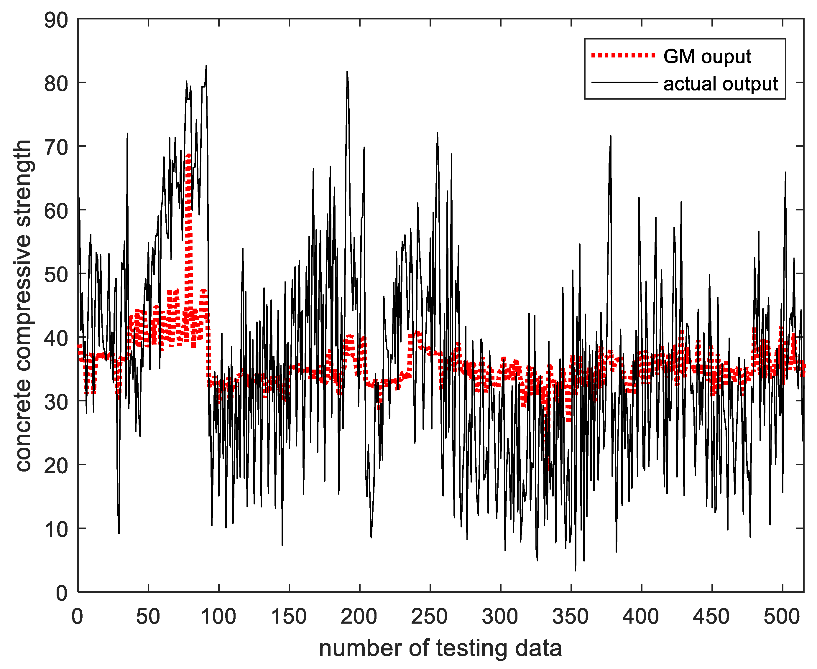
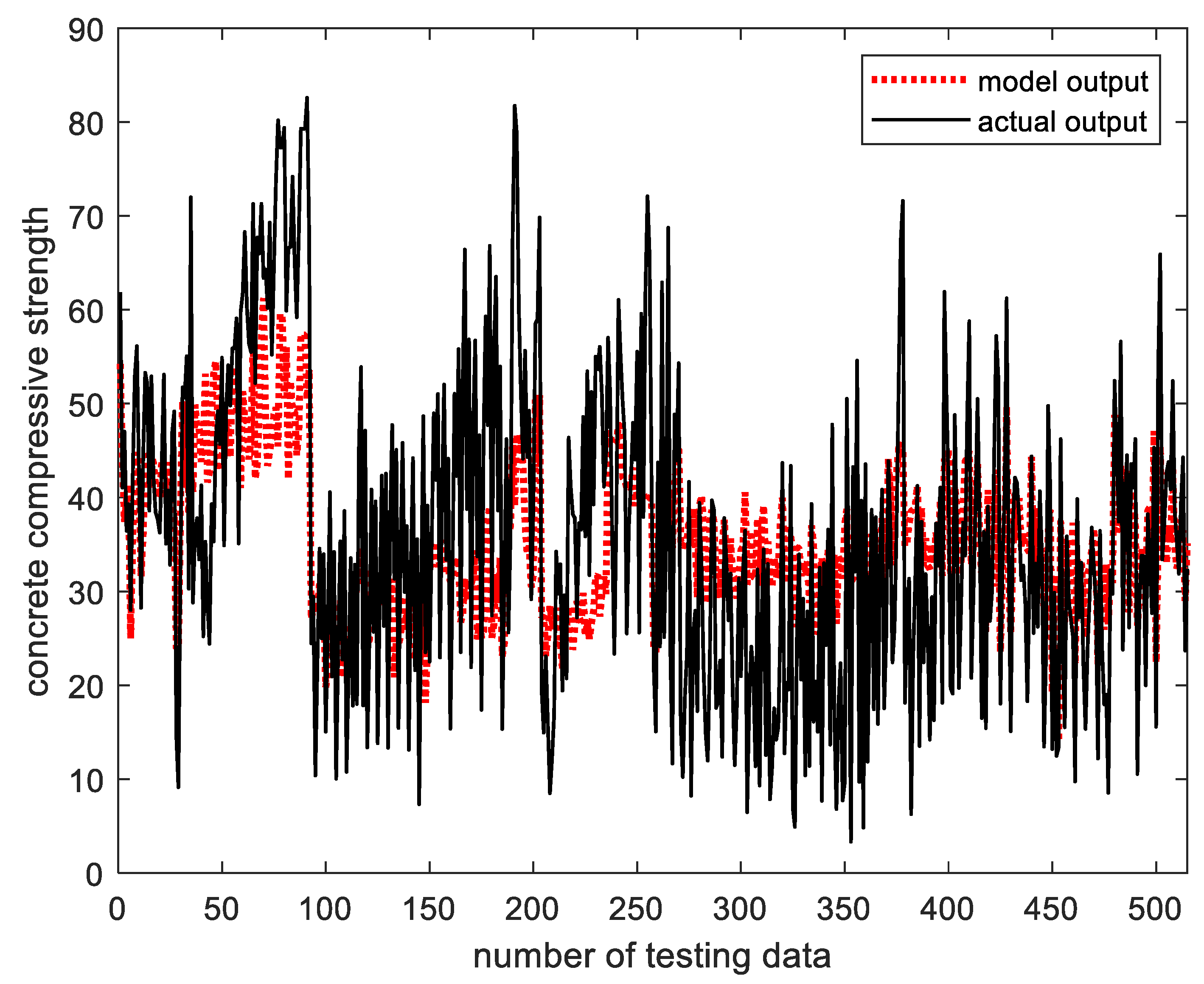
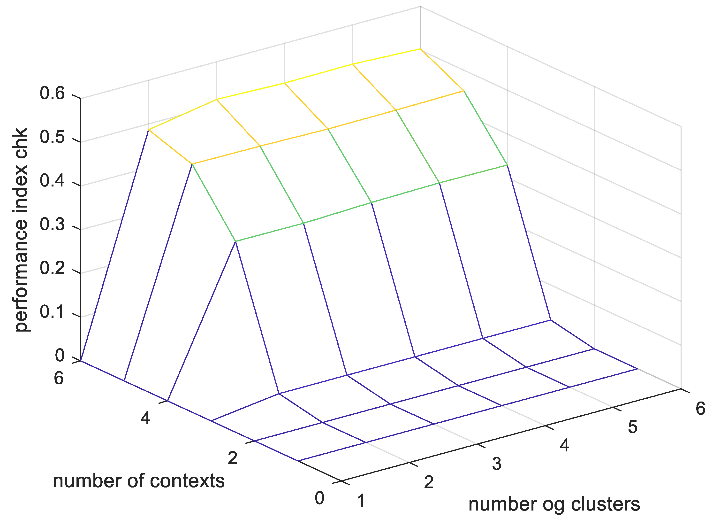
To verify the feasibility of the proposed method, an experiment was conducted using the concrete compressive strength data, a benchmarking database. To evaluate the performance of each particle model, we used a performance index using the scalability and specificity that we consider when generating rational information particles. As a result of the experiment, it was confirmed that the proposed methods were superior to the existing particle models.

In the future, based on the rational information particle generation principle, we plan to conduct research on generating various types of information particles and optimally allocating information particles created in the input space and output space.

References

1. Cazarez, R.L.U.; Diaz, N.G.; Equigua, L.S. Multi-layer adaptive fuzzy inference system for predicting student performance in online higher education. IEEE Lat. Am. Trans. 2021, 19, 98–106. [Google Scholar] [CrossRef]
2. Yeom, C.U.; Kwak, K.C. Performance comparison of ANFIS models by input space partitioning methods. Symmetry 2018, 10, 700. [Google Scholar] [CrossRef] [Green Version]
3. Ishak, K.E.H.K.; Ayoub, M.A. Predicting the efficiency of the oil removal from surfactant and polymer produced water by using liquid-liquid hydrocyclone comparison of prediction abilities between response surface methodology. IEEE Access 2019, 7, 179605–179619. [Google Scholar] [CrossRef]
4. Elbaz, K.; Shen, S.L.; Sun, W.J.; Yin, Z.Y.; Zhou, A. Prediction model of shield performance during tunneling via incorporating improved particle swarm optimization into ANFIS. IEEE Access 2020, 8, 39659–39671. [Google Scholar] [CrossRef]
5. Saucedo, J.A.M.; Hemanth, J.D.; Kose, U. Prediction of electroencephalogram time series with electro-search optimization algorithm trained adaptive neuro-fuzzy inference system. IEEE Access 2019, 7, 15832–15844. [Google Scholar] [CrossRef]
6. Alreshoodi, M.; Danish, E.; Woods, J.; Fernando, A.; Alwis, C.D. Prediction of perceptual quality for mobile video using fuzzy inference systems. IEEE Trans. Consum. Electron. 2015, 61, 546–554. [Google Scholar] [CrossRef] [Green Version]
7. Sahoo, S.; Panda, S.K.; Pratihar, D.K.; Mukhopadhyay, S. Prediction of step length using neuro-fuzzy approach suitable for prosthesis control. IEEE Trans. Instrum. Meas. 2020, 69, 5658–5665. [Google Scholar] [CrossRef]
8. Loung, T.H.L.; Tran, M.T.; Tran, T.N.; Le, H.S.; Nguyen, L.G.; Vo, T.N.N.; Pham, V.H. A new complex fuzzy inference system with fuzzy knowledge graph and extensions in decision making. IEEE Access. 2020, 8, 164899–164921. [Google Scholar]
9. Ai, C.; Jia, L.; Hong, M.; Zhang, C. Short-term road speed forecasting based on hybrid RBF neural network with the aid of fuzzy system-based techniques in urban traffic flow. IEEE Access 2020, 8, 69461–69470. [Google Scholar] [CrossRef]
10. An, J.; Fu, L.; Chen, W.; Zhen, J. A novel fuzzy-based convolutional neural network method to traffic flow prediction with uncertain traffic accident information. IEEE Access 2019, 7, 20708–20722. [Google Scholar] [CrossRef]
11. Yeom, C.U.; Kwak, K.C. Adaptive neuro-fuzzy inference system predictor with an incremental tree structure based on a context-based fuzzy clustering approach. Appl. Sci. 2020, 10, 8495. [Google Scholar] [CrossRef]
12. Parsapoor, M.; Bilstrupo, U.; Svensson, B. Forecasting solar activity with computational intelligence models. IEEE Access 2018, 6, 70902–70909. [Google Scholar] [CrossRef]
13. Kannadasan, K.; Edla, D.R.; Yadav, M.H.; Bablani, A. Intelligent-ANFIS model for predicting measurement of surface roughness and geometric tolerances in three-axis CNC milling. IEEE Trans. Instrum. Meas. 2020, 69, 7683–7694. [Google Scholar] [CrossRef]
14. Guo, H.; Zeng, W.; Shi, Y.; Deng, J.; Zhao, L. Kernel granger causality based on back propagation neural network fuzzy inference system on fMRI data. IEEE Trans. Neural Syst. Rehabil. Eng. 2020, 28, 1049–1058. [Google Scholar] [CrossRef]
15. Hwang, Y.; Kang, B.; Kim, W. Motion cue-based sudden pedestrian behavior prediction using fuzzy inference. IEEE Access 2021, 9, 135245–135255. [Google Scholar] [CrossRef]
16. Ding, Y.; Yang, S.; Chen, Y.; Long, Q.; Wei, J. Explaining and predicting mobile government microblogging services participation behaviors a SEM-neural network method. IEEE Access 2019, 7, 39600–39611. [Google Scholar] [CrossRef]
17. Ibragimov, B.; Toesca, D.A.S.; Yuan, Y.; Koong, A.C.; Chang, D.T.; Xing, L. Neural networks for deep radiotherapy dose analysis and prediction of liver SBRT outcomes. IEEE J. Biomed. Health Inform. 2019, 23, 1821–1833. [Google Scholar] [CrossRef]
18. Jia, T.; Yan, P. Predicting citywide road traffic flow using deep spatiotemporal neural networks. IEEE Trans. Intell. Transp. Syst. 2020, 22, 3101–3111. [Google Scholar] [CrossRef]
19. Wu, Q.; Jiang, Z.; Hong, K.; Liu, H.; Yang, L.T.; Ding, J. Tensor-based recurrent neural network and multi-modal prediction with Its applications in traffic network management. IEEE Trans. Netw. Serv. Manag. 2021, 18, 780–792. [Google Scholar] [CrossRef]
20. Bouda, M.; Krishna, G.; Krystofik, J.; Oda, S.; Palacharla, P. Towards vendor-agnostic real-time optical network design with extended Kalman state estimation and recurrent neural network machine learning Invited. J. Opt. Commun. Netw. 2021, 13, B21–B34. [Google Scholar] [CrossRef]
21. Liu, Y.T.; Lin, Y.Y.; Wu, S.L.; Chuang, C.H.; Lin, T.C. Brain dynamics in predicting driving fatigue using a recurrent self-evolving fuzzy neural network. IEEE Trans. Neural Netw. Learn. Syst. 2015, 27, 347–360. [Google Scholar] [CrossRef] [PubMed]
22. Dumas, T.; Roumy, A.; Guillemot, C. Context-adaptive neural network-based prediction for image compression. IEEE Trans. Image Processing 2019, 29, 679–693. [Google Scholar] [CrossRef] [PubMed] [Green Version]
23. Lin, J.W.; Chao, C.T.; Chiou, J.S. Determining neuronal number in each hidden layer using earthquake catalogues as training data in training an embedded back propagation neural network for predicting earthquake magnitude. IEEE Access 2018, 6, 52582–52597. [Google Scholar] [CrossRef]
24. Pedrycz, W.; Vasilakos, A.V. Linguistic models and linguistic modeling. IEEE Trans. Syst. Man Cybern. Part B 1999, 29, 745–757. [Google Scholar] [CrossRef] [PubMed]
25. Zhou, P.; Xu, Z.; Song, C.; Shao, Z. Long-term hybrid prediction method based on multiscale decomposition and granular computing for oxygen supply network. Comput. Chem. Eng. 2021, 153, 107442. [Google Scholar] [CrossRef]
26. Hmouz, R.A.; Pedrycz, W.; Balamash, A.S.; Morfeq, A. Hierarchical system modeling. IEEE Trans. Fuzzy Syst. 2017, 26, 258–269. [Google Scholar] [CrossRef]
27. Pedrycz, W.; Homenda, W.; Jastrzebska, A.; Yu, F. Information granules and granular models selected design investigations. In Proceedings of the 2020 IEEE International Conference on Fuzzy Systems (FUZZ-IEEE), Glasgow, UK, 19–24 July 2020. [Google Scholar]
28. Liu, Y.; Zhao, J.; Wang, W.; Pedrycz, W. Prediction intervals for granular data streams based on evolving type-2 fuzzy granular neural network dynamic ensemble. IEEE Trans. Fuzzy Syst. 2020, 29, 874–888. [Google Scholar] [CrossRef]
29. Wang, S.; Pedrycz, W. Robust granular optimization a structured approach for optimization under integrated uncertainty. IEEE Trans. Fuzzy Syst. 2014, 23, 1372–1386. [Google Scholar] [CrossRef]
30. Zhu, X.; Pedrycz, W.; Li, Z. A development of granular input space in system modeling. IEEE Trans. Cybern. 2019, 51, 1639–1650. [Google Scholar] [CrossRef]
31. Truong, H.Q.; Ngo, L.T.; Pedrycz, W. Advanced fuzzy possibilistic C-means clustering based on granular computing. In Proceedings of the 2016 IEEE International Conference on Systems, Man, and Cyberneticx, Budapest, Hungary, 9–12 October 2016. [Google Scholar]
32. Zuo, H.; Zhang, G.; Pedrycz, W.; Behbood, V.; Lu, J. Granular fuzzy regression domain adaptation in Takagi-Sugeno fuzzy models. IEEE Trans. Fuzzy Syst. 2017, 26, 847–858. [Google Scholar] [CrossRef]
33. Hu, X.; Pedrycz, W.; Wang, X. Granular fuzzy rule-Bbased models a study in a comprehensive evaluation and construction of fuzzy models. IEEE Trans. Fuzzy Syst. 2016, 25, 1342–1355. [Google Scholar] [CrossRef]
34. Zhao, J.; Han, Z.; Pedrycz, W.; Wang, W. Granular model of long-term prediction for energy system in steel industry. IEEE Trans. Cybern. 2015, 46, 388–400. [Google Scholar] [CrossRef]
35. Bezdek, J.C. Pattern Recognition with Fuzzy Objective Function Algorithms; Springer: Berlin/Heidelberg, Germany, 1981; ISBN 0-306-40671-31. [Google Scholar]
36. Silva, L.; Moura, R.; Canuto, A.M.P.; Santiago, R.H.N.; Bedregal, B. An interval-based framework for fuzzy clustering applications. IEEE Trans. Fuzzy Syst. 2015, 23, 2174–2187. [Google Scholar] [CrossRef]
37. Pedrycz, W. Conditinal fuzzy C-means. Pattern Recognit. Lett. 1996, 17, 625–632. [Google Scholar] [CrossRef]
38. Pedrycz, W. Conditional fuzzy clustering in the design of radial basis function neural networks. IEEE Trans. Neural Netw. 1998, 9, 601–612. [Google Scholar] [CrossRef] [PubMed]
39. Gustafuson, D.E.; Kessel, W.C. Fuzzy clustering with a fuzzy covariance matrix. In Proceedings of the 1978 IEEE Conference on Decision and Control inclusing the 17th Symposium on Adaptive Precesses, San Diego, CA, USA, 10–12 January 1979. [Google Scholar]
40. Babuska, R. Fuzzy Modeling for Control; Kluwer Academic Publishers: Dordrecht, The Netherlands, 1998. [Google Scholar]
41. Babuska, R.; van der Veen, P.J.; Kaymak, U. Improved covariance estimation for Gustafuson-Kessel clustering. In Proceedings of the 2002 IEEE International Conference on Fuzzy Systems, Honolulu, HI, USA, 12–17 May 2002; pp. 1081–1085. [Google Scholar]
42. Nguyen, T.T.; Pham, X.C.; Liew, A.W.C.; Pedrycz, W. Aggregation of classifiers a justifiable information granularity approach. IEEE Trans. Cybern. 2018, 49, 2168–2177. [Google Scholar] [CrossRef] [PubMed] [Green Version]
43. Zhang, B.; Pedrycz, W.; Wang, X.; Gacek, A. Design of interval type-2 information granules based on the principle of justifiable granularity. IEEE Trans. Fuzzy Syst. 2020, 29, 3456–3469. [Google Scholar] [CrossRef]
44. Wang, D.; Pedrycz, W.; Li, Z. Granular data aggregation an adaptive principle of the justifiable granularity approach. IEEE Trans. Cybern. 2018, 49, 417–426. [Google Scholar] [CrossRef]
45. Wang, D.; Pedrycz, W.; Li, Z. A two-phase development of fuzzy rule-based model and their analysis. IEEE Access 2019, 7, 80328–80341. [Google Scholar] [CrossRef]
46. Pedrycz, W.; Wang, X. Designing fuzzy sets with the use of the parametric principle of justifiable granularity. IEEE Trans. Fuzzy Syst. 2015, 24, 489–496. [Google Scholar] [CrossRef]
47. Zhang, B.; Pedrycz, W.; Fayek, A.R.; Gacek, A.; Dong, Y. Granular aggregation of fuzzy rule-based models in distributed data environment. IEEE Trans. Fuzzy Syst. 2020, 29, 1297–1310. [Google Scholar] [CrossRef]
48. Lu, W.; Wang, D.; Pedrycz, W.; Zhang, L.; Yang, J.; Liu, X. Granular fuzzy modeling for multidimensional numeric data A layered approach based on hyperbox. IEEE Trans. Fuzzy Syst. 2018, 27, 775–789. [Google Scholar] [CrossRef]
49. Zhang, B.; Dong, Y.; Feng, X.; Pedrycz, W. Maximum fuzzy consensus feedback mechanism with minimum cost and private interest in group decision-making. IEEE Trans. Fuzzy Syst. 2020, 29, 2689–2700. [Google Scholar] [CrossRef]
50. Wang, L.; Han, Z.; Pedrycz, W.; Zhao, J. A granular computing-based hybrid hierarchical method for construction of long-term prediction intervals for gaseous system of steel industry. IEEE Access 2020, 8, 63538–63550. [Google Scholar] [CrossRef]
51. Pedrycz, W.; Hmouz, R.A.; Balamash, A.S.; Morfeq, A. Hierarchical granular clustering an emergence of information granules of higher type and higher order. IEEE Trans. Fuzzy Syst. 2015, 23, 2270–2283. [Google Scholar] [CrossRef]
52. Siddique, N.; Adeli, H. Computational Intelligence: Synergies of Fuzzy Logic, Neural Networks and Evolutionary Computing; John Wiley & Sons Ltd.: Oxford, UK, 2013. [Google Scholar]
53. Freedman, D.A. Statistical Models: Theory and Practice; Cambrige University Press: Cambrige, UK, 2009. [Google Scholar]
54. Siegelmann, H.T.; Sontag, E.D. Turing computability with neural nets. Appl. Math. Lett. 1991, 4, 77–80. [Google Scholar] [CrossRef] [Green Version]
55. Broomhead, D.S.; Lowe, D. Multivariable functional interpolation and adaptive networks. Complex Syst. 1988, 2, 321–355. [Google Scholar]
56. Broomhead, D.S.; Lowe, D. Radial Basis Functions, Multi-Variable Functional Interpolation and Adaptive Networks; Technical Report; RSRE (Royal Signals & Radar Establishment): Malvern, UK, 1988; Volume 4148. [Google Scholar]
57. UCI Machine Learning Repository, Concrete Compressive Strength Data Set. Available online: https://archive.ics.uci.edu/ml/datasets/Concrete+Compressive+Strength (accessed on 16 February 2022).
58. Available online: https://www.cs.toronto.edu/~delve/data/boston/bostonDetail.html (accessed on 16 February 2022).
Figure 1. Context-based fuzzy clustering and interval-based fuzzy clustering concept: (a) context-based fuzzy clustering; (b) interval-based fuzzy clustering.
Applsci 12 03154 g001
Figure 2. Comparison of clusters created in fuzzy clustering and context-based fuzzy clustering: (a) presents normal fuzzy clustering; (b) context-based fuzzy clustering.
Applsci 12 03154 g002
Figure 3. Comparison of clusters created with fuzzy and GK clustering: (a) fuzzy clustering; (b) GK clustering.
Applsci 12 03154 g003
Figure 4. Concepts of coverage and specificity for creating rational IGs: (a) concept of coverage; (b) concept of specificity.
Applsci 12 03154 g004
Figure 5. Trade-off relationship between IG coverage and specificity.
Applsci 12 03154 g005
Figure 6. Structure of a fuzzy-based granular model.
Applsci 12 03154 g006
Figure 7. Data set with two features in the output space.
Applsci 12 03154 g007
Figure 8. Comparison of clusters created in GK and CGK clustering: (a) general GK clustering; (b) context-based GK clustering.
Applsci 12 03154 g008
Figure 9. CGK clustering concept.
Applsci 12 03154 g009
Figure 10. CGK-based granular model structure.
Applsci 12 03154 g010
Figure 11. Granular model with a hierarchical structure.
Applsci 12 03154 g011
Figure 12. Linear regression model concept.
Applsci 12 03154 g012
Figure 13. Neural network structure.
Applsci 12 03154 g013
Figure 14. Radial basis function network structure.
Applsci 12 03154 g014
Figure 15. Structure of a CGK granular model with an aggregated structure.
Applsci 12 03154 g015
Figure 16. Comparison of the output value of the existing GM with the actual output value (context is created equally, the number of contexts = 6, the number of clusters = 6).
Applsci 12 03154 g016
Figure 17. GM’s performance index for validation data (context equally generated, number of contexts = 6, number of clusters = 6).
Applsci 12 03154 g017
Figure 18. Comparison of the output value of the existing CGK-GM with the actual output value (context is created equally, the number of contexts = 6, the number of clusters = 4).
Applsci 12 03154 g018
Figure 19. CGK-GM’s performance index for validation data (context equally generated, number of contexts = 6, number of clusters = 4).
Applsci 12 03154 g019
Figure 20. Comparison of the output value of the existing AGM with the actual output value (context is created equally, the number of contexts = 6, the number of clusters = 6).
Applsci 12 03154 g020
Figure 21. AGM’s performance index for validation data (context equally generated, number of contexts = 6, number of clusters = 6).
Applsci 12 03154 g021