An Accurate State Visualization of Multiplexed and PWM Fed Peripherals in the Virtual Simulators of Embedded Systems

Abstract

A method of precise and real-like embedded systems peripherals visualization in virtual simulations is presented in the article. For high frequency peripheral inputs, blended graphics of real-look representations of peripherals are used, allowing for an accurate visualization with consideration of their input signal nature based on PWM and multiplexing schemes. An accurate simulator of a didactic embedded system called MKD-51 is introduced as a plug in for Keil μVision IDE. A comparison with a real microprocessor system using multiplexing seven-segment LED modules as well as LED bar fed by PWM is shown. The achieved quantity results are included to illustrate compliance with real devices and improvements in visualization accuracy due to applying additional blending mapping function. Brightness estimation differences of LED visualization compared to a real device are at a single percentage level for seven-segment multiplexed modules.

1. Introduction

The virtual simulators of real embedded systems are widely used nowadays composing so called virtual laboratories [1]. Following [1] “a virtual laboratory is a real laboratory at an university with corresponding laboratory devices, receptacles and substances, that can be observed by tele-users with the help of cameras and can be remote controlled with robots”. Also “textual web-pages with integrated animations, Java-Applets or Shockwave-Movies, that are used for simulation of laboratory equipment or processes, are frequently named virtual laboratories”. Virtual laboratories are frequently used nowadays allowing for virtual or fast prototyping [2]. They can be used for complex systems of different nature such as electrical, mechanical, thermal, software, etc. [2] and both for developing software for embedded systems in industry [3] as well as in didactic areas [4,5]. In [3] the process of building the concrete simulation, a system for an embedded board that can run the real software can be determined. [4] describes the design and implementation of a simulation-based education package for embedded system courses. The described solutions help to develop a microprocessor system embedded software quickly and efficiently.

This is even more important these days, when remote work, without access to physical devices, is more than common due to the COVID 19 pandemic [6,7]. According to [8], more than 850 million of children and young people were being kept away from schools and universities, with national closures active in 102 countries and local closures in 11 others. The authors propose the emergency remote teaching (ERT) technique using Microsoft Teams and analyze the satisfaction of the students using it. The virtual simulator of an embedded system presented in our article was also accompanied by MS Teams in the didactic process.

Access to the simulators of embedded systems has many advantages. Among them, the protection of hardware [9] (especially MCU main boards, actuators and controlled objects), avoidance of repeated programming of memories (the process is slow and can lead to wear out of the hardware) and high speed and accuracy of software running process seems to be the most important [10]. There are also some drawbacks of the virtual simulators. The main drawback seems to be the simulation itself which that leads to the feeling that it is not the reality. That is why much effort must be made to accurately emulate the peripheral hardware devices seen or touched by the user.

In real hardware, utilization of a pulse width modulation (PWM) fed and multiplexed peripherals are the most basic techniques, and they are used frequently [11]. Unfortunately, if PWM or multiplexing techniques are used in conjunction with peripherals that are intended for human handling, a proper reception of their operation is based on human perception inertia. The proper visualization of this situation in a virtual simulator, regarding to graphical representation of visualized peripherals on the monitor, can be very difficult.

In this article, a simple and very effective algorithm which considers high rate dynamic changes of visualized peripherals is introduced along with exemplary simulator of the MKD-51 didactical system used inside the Keil μVision IDE as a plugin [12]. The objective of the paper is to present an algorithm for visualizing peripherals fed by PWM or multiplexed in their real-like representation regardless of its input signal frequency. This approach represents a novelty in the field of virtual simulators.

This work is divided into the following sections. In Section 2, hardware details of the MKD-51 didactic system and its virtual simulator are presented. In Section 3, the mathematical and algorithmic background is shown. In Section 4 and Section 5, the results and discussion are presented, respectively. Section 6, concludes the paper.

2. Materials

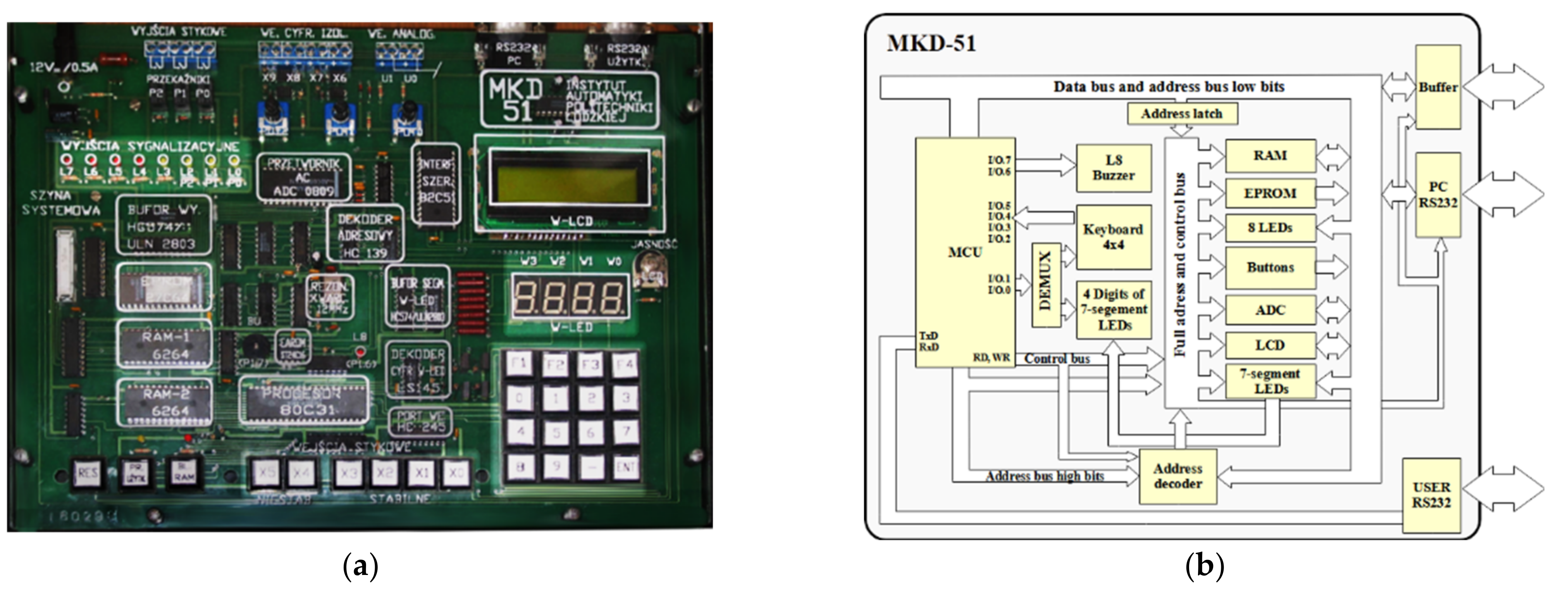
2.1. The MKD-51 Didactic System

At the Lodz University of Technology, in the Institute of Automatic Control [13], a number of virtual simulators for the purpose of embedded system programming teaching are used. One of them is especially useful for early-stage learning of peripherals handling that are used in real embedded systems. The MKD-51 didactic system [14], shown in Figure 1, includes all of those basic peripherals in the simplest possible form - switches, matrix keyboard, LEDs, seven-segment displays, alphanumeric LCD, and potentiometers with an external ADC.

All of those peripherals are handled both directly from MCU I/O ports and through an external bus, covering the basis of peripheral programming methods. The hardware structure was intentionally left in a low scale of integration to show memories, address decoders, and additional I/O ports, gates, and buffers. Those are all of the electronic components that students should be aware of, especially given that every modern microcontroller [15] or Programmable System on Chip (PSoC) [16] has hidden them inside a single chip.

2.2. The MKD51 SIM—A Virtual Simulator of Peripherals

Access to the reliable virtual embedded system simulator is very important in didactics. Students often need much more time to practice and debug their programming tasks, and time spent at university is insufficient in many situations. Also nowadays, during the COVID 19 pandemic, lots of didactic laboratories were transferred into a remote form. This has encouraged us to develop a virtual simulator called MKD-51 SIM (Figure 2) which requires exactly the same programming methods as the real MKD-51 system (described in Section 2.1). The compatibility of the virtual simulator with the real hardware is basically 100%. This leads very often to situations wherein students prefer to use virtual simulator even in class hours instead of real devices.

The simulator guarantees a high accuracy of all peripherals’ behavior. Keys can be pushed, both with a mouse or PC keyboard, potentiometers can be rotated to produce voltage inputs to the ADC, LEDs can be driven with high frequency inputs, seven-segment LED modules can be multiplexed, and alphanumeric LCDs can be programmed in the same way as real ones. The simulator has one additional component that is not present in the real platform, namely a graphical LCD operating in RGB888 mode with resolution of 64 × 128 pixels.

2.3. Keil μVision IDE

There are many good integrated development environments (IDE) for embedded systems software development. Some of them can use external virtual hardware simulators, but only a few have a strong support for simulating processors and microcontrollers inside IDE. This support is very convenient, since a virtual embedded system simulator has to implement only specific peripherals behavior for the specific hardware project. On the market, there are a few well known IDEs with internal support of MCUs. These include Microchip Studio [17], earlier versions of Code Composer Studio [18] (now without internal CPU simulation support), and Keil μVision [19]. The last one allows one to expand the internal simulator capabilities through the simple but very effective plugin system quite easily [20]. The virtual simulator presented in this paper was prepared as such a plugin and can run directly under control of μVision IDE (Figure 3).

3. Methods

3.1. The Problem Formulation

A typical PC monitor is able to show graphical information at a typical rate in a range from 50 Hz to 200 Hz. This directly limits the rate of simulated visualization parts in the form which represents their physical appearance. For example, the attempt to change the LED state with a rate of 400 Hz in the monitor or a refreshing rate of 200 Hz would lead to permanent LED OFF or ON state visualization, depending on the LED initial state. This problem will also occur when the visualization changing time moment will be improperly taken even for lower frequencies than the monitor refresh rate. The visual analysis of the achieved results in the virtual simulator, made by developer, could lead to wrong conclusions and inability to locate potentially not working part of the software.

The problem could also be defined in terms of the aliasing phenomena and spectral leakage in digital signal processing [21]. In such an approach, the visual modifications of simulated peripherals should change less frequently than half of the monitor refresh rate and their graphical representation changing time should be its multiple. The main issue here is that for a certain and desirable input signal frequency to be shown in the virtual simulator through the behavior of controlled peripheral, increasing the monitor refresh rate is rather impossible.

3.2. An Algorithm for Visualizing Peripherals Fed by High Rate Input Signal

A proper graphical visualization of simulated parts (in their real appearance) needs to analyze input signals and be able to show their influence on peripheral (and, even then, if the input signal changes are more frequent than monitor refreshing rate). Solving this issue is possible using a proposed algorithm presented in Figure 4.

The algorithm principle is to take two different actions regarding to signal changes nature. In the case of low frequency or no change of an input signal for a given time threshold, a graphical representation of the peripheral should be just drawn on the screen. In the opposite case, a mean value should be calculated and properly proposed. In the case of PWM signals, this could be a width of its active state (Figure 4). The time threshold T_h, in the simplest approach, can be calculated as simply as:

$$T_h=\frac{1}{f_r},$$

(1)

where f_r is a frequency of monitor refresh rate. For most simulators and typical peripherals. T_h can be assumed to be 10 ms.

3.3. Experimental Setup

For verification purposes of peripheral visualization results, the photos for different expositions of real MKD-51 peripherals were taken. The system was executing a specially prepared program (Appendix A) which was also run in the virtual simulator under Keil μVision IDE in the same form. Results of the simulator visualizations were acquired using screenshots of corresponding peripherals. Both types of obtained images were normalized and compared using procedure described in the following sections.

3.4. Calculating the Peripheral Image Corresponding to the Averaged Input Signal

The important part of proposed algorithm is to calculate resultant image. This is based on three components: two real peripheral appearances in two of their states and the time moment of triggering these two states. The formula for visualization image calculation is a linear combination between those two images in proportions dependent of an input signal. This is very well know image blending technique [22] and it is given by:

$$Im{g}_{result}\left(x,y\right)=Im{g}_{stat{e}_1}\left(x,y\right) · c_{stat{e}_1}+Im{g}_{stat{e}_2}\left(x,y\right) · c_{stat{e}_2}$$

(2)

where c_state coefficients are closely related to the distance of the average input signal i_avg to the boundaries of its graphical peripheral representations for i_img1 and i_img2 inputs:

$$c_{stat{e}_1}=\frac{|i_{img2}-i_{avg}|}{|i_{img1}-i_{img2}|}, c_{stat{e}_2}=\frac{|i_{img1}-i_{avg}|}{|i_{img1}-i_{img2}|}$$

(3)

The correct peripheral visualization image, prepared according to Equations (2) and (3), assumes that the real appearance is changing gradually along the input signal between two captured peripheral image representations. This is especially true for brightness perception of LED fed by PWM with pulse width that corresponds to average input value and LED displays controlled using multiplexing. If the peripheral behavior does not meet this assumption, any nonlinear function f_map can be applied to provide a visualization that corresponds to the reality. In such a case image calculation can be rewritten as:

$$\begin{gathered} Im{g}_{result}\left(x,y\right)=Im{g}_{stat{e}_1}\left(x,y\right) · c_{map}+Im{g}_{stat{e}_2}\left(x,y\right) · \left(1-c_{map}\right) \\ where c_{map}=f_{map}\left(c_{stat{e}_1}\right) \end{gathered}$$

(4)

4. Results

4.1. Multiplexed Seven-Segment LED Displays Visualization

For analysis purposes, a special multiplexing scheme of seven-segment LED displays was applied. There was a switching sequence: W0, W0, W0, W0, W1, W1, W2, with period of 2 ms. The result of such a multiplexing is shown in Figure 5a,b.

The LCD display images were normalized for analysis by histogram stretching [23] with the results shown in Figure 5c,d. The mean value and median of statistics distributions were gathered in

Table 1. Comparison of multiplexed digits images statistics.

Analyzed Statistics	W2 Digit	W1 Digit	W0 Digit
MKD-51 brightness mean MKD-51 SIM brightness mean	0.06	0.18	0.25
	0.05	0.16	0.25
MKD-51 brightness median MKD-51 SIM brightness median	0.05	0.17	0.29
	0.06	0.18	0.29

for every visualized digit separately. It should be emphasized that from analyzed histograms, the zeroth brightness (black background) were removed in order not to distort the results [24].

4.2. Visualization of the LEDs Fed by PWM in the Simulator

Similarly, to the seven-segment LEDs display case presented in Section 4.1, a dedicated algorithm, implemented in C language (Appendix A), was applied to drive LEDs with different pulse widths to verify the MKD-51 SIM. The LED bar consist of four red diodes and four yellow ones. Each color behaves differently, so they were tested separately. Pulse widths of 0%, 10%, 30%, and 100% were applied for diodes L7-L4 and L3-L0. The time period of PWM was set to 5 ms which gives a frequency of 200 Hz with 10 points of PWM resolution. Results achieved in real MKD-51 system and its virtual simulator are shown in Figure 6a,c.

Images of controlled LEDs are not suitable for direct comparison. To be able to compare them, the series of images processing is needed to normalize them in terms of:

• Any non-corresponding to LEDs brightness image parts were removed;
• Image histograms were stretched to trim brightness below graphical representation of 0% of diode PWM and to achieve comparable parts of diodes graphical representation for 100% of PWM;
• The brightness levels from 0 to 0.3 were removed from images to avoid shadows and afterglows influence on results [25].

The normalization procedure allowed on to achieve the images shown in Figure 6b,d. In case of LED brightness analysis, it can be easily noticed that the size of their graphical representation can be a supplementary information. Therefore, a nonzero pixel ratio of analyzed LED to the LED driven with 100% of PWM was acquired and calculated. The results were gathered and are shown in

Table 2. Comparison of LED normalized images statistics.

Analyzed Feature	L6	L5	L4	L2	L1	L0
MKD-51 non-zero pixels ratio MKD-51 SIM non-zero pixels ratio	0.47	0.75	1	0.44	0.78	1
	0.42	0.85	1	0.13	0.43	1
MKD-51 brightness mean MKD-51 SIM brightness mean	0.48	0.62	0.63	0.41	0.73	0.8
	0.19	0.27	0.81	0.15	0.19	0.89
MKD-51 brightness median MKD-51 SIM brightness median	0.46	0.58	0.58	0.41	0.82	0.98
	0.2	0.28	0.81	0.12	0.2	0.9

.

4.3. LED Brightness Mapping for Accurate Visualization

Results of LEDs visualization presented in previous subchapter are not satisfying. To achieve more accurate visualization, a simple compensation function can be used to adjust virtual LED brightness. The function was proposed is in the following form:

$$f_{map}\left(V\right)=1+a · e^{-V · b}$$

(5)

where a and b coefficients were picked empirically as values of 4 and 5. The comparative results with the use of compensation formula and for different PWM duty cycle schemes are shown in Figure 7.

The statistics of normalized images histograms for single LEDs were calculated using perceptual scale. The results are shown in

Table 3. Comparison of LED normalized images statistics with (W) and without (N) brightness compensation for 0%, 10%, 30%, and 100% duty cycle of PWM scheme.

Analyzed Feature	L6	L5	L4	L2	L1	L0
MKD-51 non-zero pixels ratio MKD-51 SIM non-zero pixels ratio W MKD-51 SIM non-zero pixels ratio N	0.47	0.75	1	0.44	0.78	1
	0.73	0.9	1	0.28	0.94	1
	0.42	0.85	1	0.13	0.43	1
MKD-51 brightness mean MKD-51 SIM brightness mean W MKD-51 SIM brightness mean N	0.48	0.62	0.63	0.41	0.73	0.8
	0.22	0.42	0.81	0.17	0.25	0.9
	0.19	0.27	0.81	0.15	0.19	0.9
MKD-51 brightness median MKD-51 SIM brightness median W MKD-51 SIM brightness median N	0.46	0.58	0.58	0.41	0.82	0.98
	0.2	0.44	0.81	0.16	0.25	0.9
	0.2	0.28	0.81	0.12	0.2	0.9

and

Table 4. Comparison of LED normalized images statistics with (W) and without (N) brightness compensation for 0%, 30%, 60%, and 100% duty cycle of PWM scheme for different photo exposure of the real MKD-51.

Analyzed Statistics	L6	L5	L4	L2	L1	L0
MKD-51 non-zero pixels ratio MKD-51 SIM non-zero pixels ratio W MKD-51 SIM non-zero pixels ratio N	0.65	0.9	1	0.73	0.95	1
	0.9	0.97	1	0.94	0.98	1
	0.85	0.95	1	0.43	0.96	1
MKD-51 brightness mean MKD-51 SIM brightness mean W MKD-51 SIM brightness mean N	0.71	0.73	0.72	0.7	0.76	0.78
	0.42	0.6	0.81	0.25	0.45	0.9
	0.27	0.54	0.81	0.19	0.32	0.9
MKD-51 brightness median MKD-51 SIM brightness median W MKD-51 SIM brightness median N	0.77	0.82	0.8	0.76	0.92	0.94
	0.44	0.59	0.81	0.25	0.44	0.9
	0.28	0.55	0.81	0.2	0.31	0.9

.

5. Discussion

An accurate visualization of graphical representation of peripheral state needs to consider two issues. The first one is a proper visualizing algorithm and the second is the method to assess achieved results. Determining the brightness of objects based on their graphical representation is a common task [26]. For the purposes of analyzing acquired graphical data, the authors adopts a simplified method based on two features of the light emitting element normalized graphic representation, namely its size expressed in non-zero pixels [27] and the basic histogram statistics [28]. The analysis of the obtained results leads to the following considerations:

• Visualizing multiplexing seven-segment LED displays is satisfyingly accurate without any additional modification to proposed visualization algorithm. After image normalization a W2 LED module brightness is almost the same, in a statistic manner, as for real hardware. The difference of statistics is at level 0.02 for the mean value and 0.01 for the median. The conclusion can be extended to results analysis without an image normalization as a comparable relation between any two LED digits brightness which are almost identical for a virtual and a real peripheral;
• Comparison of real and virtual LED bar visualization accuracy cannot be carried out reliable using only histogram statistics. This is caused by size changing of real image representation of LEDs along with their brightness. An additional feature is needed, which was taken into account;
• More accurate result analysis can introduce the resulting compound brightness factor as a multiplication of relative image size, expressed as a relation of non-zero pixels counts of two LEDs (analyzed and fully driven), and chosen histogram statistics. Based on this, the set of factors can be achieved that are more suitable for direct comparison (Figure 8 and Figure 9).

• As shown in Figure 8 and Figure 9, the proposed algorithm of LEDs visualization is following changes in controlled LED perceived brightness. In the case of implemented algorithm without additional brightness compensation, its perceived brightness was considered to be far insufficient in receipt. Using additional f_map function, correcting visualized LED brightness was carried out. Although analysis of relative factors indicate that the compensation could be more intensive, final visualization results perceived by the human eye deemed sufficient. The a and b correction factors, chosen in the f_map function, have been selected empirically in order to obtain more appropriate visual representation of simulated peripheral behavior. They were not selected analytically or optimally, which may be the subject of potential further research, as well as the class of f_map functions modifying brightness, which may be more closely related to the visualized type of LED or another peripheral object.

The photos of the actual hardware being analyzed in the article were not taken in identical conditions. Moreover, for a more reliable, comprehensive, and robust [29] assessment of proposed solutions, they should not be taken in stationary manner and should even emphasize various features of the object [30]. This means that the chosen methods should not rely on the stationary nature of the image acquiring parameters. One solution to this issue is an image normalization [31], which was performed according to instructions given in the article criteria. The data prepared in this way can be compared in more reliable manner, and this has been carried out in this article.

6. Conclusions

The proposed method of embedded systems peripherals visualization and obtained research results confirm that a correct graphic representation of peripheral systems, consistent with the visual perception of the user of real hardware, can be achieved in virtual simulators. The presented algorithm can be successfully used as a component of modern simulators of embedded systems that need to reproduce a visual behavior of LEDs controlled by both PWM and multiplexed methods with the greatest possible precision. The brightness estimation coefficients relative differences of LED visualization compared to real device are at 1% for median and 2% for mean values in the case of simulating seven-segment modules controlled by multiplexing. Comparing LEDs brightness fed by PWM signal with the use of indicative brightness estimates was less accurate due to the additional image feature in the virtual simulator (in the form of white rings around a LED) that caused less relative estimated image brightness of a whole graphical LED representation. Visualization accuracy calculated under those assumptions is between 10 to 30% depending on LED color and PWM duty cycle. The discussed method is simple to implement and does not require large computational resources. It can be used for developing virtual simulators operating in the real time. The MKD-51 SIM simulator presented in the paper proves that such a solution can be successfully used as component that expands the capabilities of modern IDE.

References

1. Scherp, A. Software development process model and methodology for virtual laboratories. In Proceedings of the 20th IASTED International Conference on Applied Informatics, Innsbruck, Austria, 18–21 February 2002. [Google Scholar]
2. Beghi, A.; Marcuzzi, F.; Martin, P.; Tinazzi, F.; Zigliotto, M. Virtual prototyping of embedded control software in mechatronic systems: A case study. Mechatronics 2017, 43, 99–111. [Google Scholar] [CrossRef]
3. Engblom, J. Using Simulation Tools for Embedded Software Development. In Proceedings of the Embedded Systems Conference, San Jose, CA, USA, 14–18 April 2008. [Google Scholar]
4. Cho, S.-Y. A virtual simulation package for Embedded System training and education. In Proceedings of the 2009 International Conference on Engineering Education (ICEED), Kuala Lumpur, Malaysia, 7–8 December 2009; pp. 72–76. [Google Scholar]
5. Cruz-Miguel, E.; Rodriguez, J.; García-Martínez, J.; Camarillo-Gómez, K.; Pérez-Soto, G. Field-programmable gate array-based laboratory oriented to control theory courses. Comput. Appl. Eng. Educ. 2019, 27, 1253–1266. [Google Scholar] [CrossRef] [Green Version]
6. Xie, W.; Yang, X.; Li, F. A virtual laboratory platform and simulation software based on web. In Proceedings of the 2008 10th International Conference on Control, Automation, Robotics and Vision, Hanoi, Vietnam, 17–20 December 2008; IEEE: Piscataway, NJ, USA, 2008; pp. 1650–1654. [Google Scholar]
7. Khant, S.; Patel, A. COVID19 remote engineering education: Learning of an embedded system with practical perspective. In Proceedings of the International Conference on Innovative Practices in Technology and Management (ICIPTM 2021), Noida, India, 17–19 February 2021. [Google Scholar]
8. Rodriguez-Segura, L.; Zamora-Antuñano, M.A.; Rodriguez-Resendiz, J.; Paredes-García, W.J.; Altamirano-Corro, J.A.; Cruz-Pérez, M.Á. Teaching Challenges in COVID-19 Scenery: Teams Platform-Based Student Satisfaction Approach. Sustainability 2020, 12, 7514. [Google Scholar] [CrossRef]
9. Engblom, J. On Hardware and Hardware Models for Embedded Real-Time Systems. In Proceedings of the IEEE Workshop on Real-Time Embedded Systems (WRTES 2001), London, UK, 3 December 2001. [Google Scholar]
10. Schnerr, J.; Bringmann, O.; Viehl, A.; Rosenstiel, W. High-performance timing simulation of embedded software. In Proceedings of the 45th annual conference on Design automation—DAC ’08, Anaheim, CA, USA, 8–13 June 2008; p. 290. [Google Scholar]
11. Lee, J.; Park, G.; Shin, J.; Lee, J.; Sreenan, C.; Yoo, S. SoEasy: A Software Framework for Easy Hardware Control Programming for Diverse IoT Platforms. Sensors 2018, 18, 2162. [Google Scholar] [CrossRef] [PubMed] [Green Version]
12. Microprocessor Systems Laboratory. Available online: http://ztchs.p.lodz.pl/index.php?www=SM (accessed on 20 February 2022).
13. Institute of Automatic Control, Lodz University of Technology. Available online: https://www.automatyka.p.lodz.pl/?lang=en (accessed on 19 February 2022).
14. Mroczek, H. Microprocessor Technique (In Polish); Lodz Uniwersity of Technology Press: Łódź, Poland, 2007; ISBN 978-83-7283-238-2. [Google Scholar]
15. Bolanakis, D.E. A Survey of Research in Microcontroller Education. IEEE Rev. Iberoam. Tecnol. de Aprendiz. 2019, 14, 50–57. [Google Scholar] [CrossRef]
16. Adi, P.D.P.; Kitagawa, A.; Sihombing, V.; Silaen, G.J.; Mustamu, N.E.; Siregar, V.M.M.; Sianturi, F.A.; Purba, W. A Study of Programmable System on Chip (PSoC) Technology for Engineering Education. J. Phys. Conf. Ser. 2021, 1899, 012163. [Google Scholar] [CrossRef]
17. Microchip Studio for AVR® and SAM Devices. Available online: https://www.microchip.com/en-us/tools-resources/develop/microchip-studio (accessed on 19 February 2022).
18. CCSTUDIO. Code Composer StudioTM Integrated Development Environment (IDE). Available online: https://www.ti.com/tool/CCSTUDIO (accessed on 19 February 2022).
19. µVision® IDE. Available online: https://www2.keil.com/mdk5/uvision/ (accessed on 19 February 2022).
20. Nayyar, A. An Encyclopedia Coverage of Compiler’s, Programmer’s & Simulator’s for 8051, PIC, AVR, ARM, Arduino Embedded Technologies. Int. J. Reconfigurable Embed. Syst. 2016, 5, 18. [Google Scholar] [CrossRef]
21. Lyons, R.G. Understanding Digital Signal. Processing; Addison Wesley Pub Co., Inc., Pearson: Boston, MA, USA, 2010; ISBN 9780137027415. [Google Scholar]
22. Popovic, V.; Afshari, H.; Schmid, A.; Leblebici, Y. Real-time implementation of Gaussian image blending in a spherical light field camera. In Proceedings of the 2013 IEEE International Conference on Industrial Technology (ICIT), Cape Town, South Africa, 25–28 February 2013; IEEE: Piscataway, NJ, USA; pp. 1173–1178.
23. Im, J.; Jeon, J.; Hayes, M.; Paik, J. Single image-based ghost-free high dynamic range imaging using local histogram stretching and spatially-adaptive denoising. IEEE Trans. Consum. Electron. 2011, 57, 1478–1484. [Google Scholar] [CrossRef]
24. Myasnikova, E.; Samsonova, M.; Kosman, D.; Reinitz, J. Removal of background signal from in situ data on the expression of segmentation genes in Drosophila. Dev. Genes Evol. 2005, 215, 320–326. [Google Scholar] [CrossRef] [PubMed]
25. Kirberger, R.M. Imaging artifacts in diagnostic ultrasound—A review. Vet. Radiol. Ultrasound 1995, 36, 297–306. [Google Scholar] [CrossRef]
26. Park, H.J.; Kim, K.B. Estimation of object location probability for object detection using brightness feature only. Int. J. Electr. Comput. Eng. 2019, 9, 5227. [Google Scholar] [CrossRef]
27. Wang, X.; Guo, Q. Enhancing computational integral imaging performance using an interpolation method based on non-zero-pixel derivation. Appl. Opt. 2010, 49, 3997. [Google Scholar] [CrossRef] [PubMed]
28. Maini, R.; Aggarwal, H. A Comprehensive Review of Image Enhancement Techniques. arXiv 2010, arXiv:1003.4053. [Google Scholar]
29. Kaur, H.; Sohi, N. A Study for Applications of Histogram in Image Enhancement. Int. J. Eng. Sci. 2017, 6, 59–63. [Google Scholar] [CrossRef]
30. Blaschke, T. Object based image analysis for remote sensing. ISPRS J. Photogramm. Remote Sens. 2010, 65, 2–16. [Google Scholar] [CrossRef] [Green Version]
31. Li, T.; Wei, L.; Hsu, W. A Multi-Pronged Evaluation for Image Normalization Techniques. In Proceedings of the 2021 IEEE 18th International Symposium on Biomedical Imaging (ISBI), Nice, France, 13–16 April 2021; IEEE: Piscataway, NJ, USA, 2021; pp. 1292–1296. [Google Scholar]
Figure 1. The MKD-51 didactic system: (a) real photo; (b) block diagram.
Applsci 12 03137 g001
Figure 2. The MKD-51 SIM running demo program.
Applsci 12 03137 g002
Figure 3. The MKD-51 virtual simulator runs under debugging process inside Keil μVision IDE.
Applsci 12 03137 g003
Figure 4. An algorithm of proper graphical visualization of peripherals in their real appearance regarding the input signal changes.
Applsci 12 03137 g004
Figure 5. The multiplexed seven-segment LED display: (a) MKD-51 photo; (b) MKD-51 SIM image; (c) normalized MKD-51 photo for analysis; and (d) normalized MKD-51 SIM image for analysis.
Applsci 12 03137 g005
Figure 6. The LED bar of MKD-51 didactic system fed by different PWM duty cycles: (a) the real MKD-51 photo; (b) the real MKD-51 photo after normalization; (c) the MKD-51 SIM image; (d) the MKD-51 SIM image after normalization.
Applsci 12 03137 g006
Figure 7. The LED bars driven with different PWMs. (a,b) The real MKD-51 photos taken with two different exposures; (c,d) MKD-51 SIM with compensation formula; (e,f) MKD-51 SIM without compensation formula; (a,c,e) LEDs driven with 0%, 30%, 60%, and 100% of PWM duty cycle; (b,d,f) LEDs driven with 0%, 10%, 30%, and 100% of PWM duty cycle;.
Applsci 12 03137 g007
Figure 8. Comparison of LED normalized compound brightness factors with (W) and without (N) brightness compensation for 0%, 10%, 30%, and 100% duty cycle of PWM scheme.
Applsci 12 03137 g008
Figure 9. Comparison of LED normalized compound brightness factors with (W) and without (N) brightness compensation for 0%, 30%, 60%, and 100% duty cycle of PWM scheme for different photo exposure of the real MKD-51.
Applsci 12 03137 g009