
Estimation of Hydrogeological Parameters by Using Pumping, Laboratory Data, Surface Resistivity and Thiessen Technique in Lower Bari Doab (Indus Basin), Pakistan


Abstract
1. Introduction
2. Materials and Methodology
3. Results and Discussion
4. Conclusions
Author Contributions
Funding
Institutional Review Board Statement
Informed Consent Statement
Data Availability Statement
Acknowledgments
Conflicts of Interest
References
- Alam, U.; Sahota, P.; Jeffrey, P. Irrigation in the Indus basin: A history of unsustainability? Water Supply 2007, 7, 211–218. [Google Scholar] [CrossRef]
- Watto, M.A. The Economics of Groundwater Irrigation in the Indus Basin, Pakistan: Tube-Well Adoption, Technical and Irrigation Water Efficiency and Optimal Allocation. Ph.D. Thesis, University of Western Australia, Perth, Australia, 2015. [Google Scholar]
- Mondal, P.; Dalai, A.K. Sustainable Utilization of Natural Resources; CRC Press: Boca Raton, FL, USA, 2017. [Google Scholar] [CrossRef]
- Yu, W.H.; Yang, Y.-C.; Savitsky, A.; Alford, D.; Brown, C. The Indus Basin of Pakistan: The Impacts of Climate Risks on Water and Agriculture; World Bank Publications: Herndon, VA, USA, 2013; Available online: http://hdl.handle.net/10986/13834 (accessed on 10 January 2022).
- Mukherjee, A. Overview of the groundwater of South Asia. In Groundwater of South Asia; Springer Science and Business Media LLC: Dordrecht, The Netherlands, 2018; pp. 3–20. Available online: https://link.springer.com/chapter/10.1007/978-981-10-3889-1_1 (accessed on 10 January 2022).
- Bakhsh, A.; Awan, Q. Water issues in Pakistan and their remedies. In Proceedings of the National Symposium on Drought and Water Resources in Pakistan, Punjab, Pakistan, 16 March 2002; pp. 145–150. [Google Scholar]
- Bakhsh, A.; Kanwar, R.S.; Pederson, C.; Bailey, T.B. N-Source Effects on Temporal Distribution of NO3-N Leaching Losses to Subsurface Drainage Water. Water Air Soil Pollut. 2007, 181, 35–50. [Google Scholar] [CrossRef]
- Saeed, M. Skimming Wells; Higher Education Commission: Islamabad, Pakistan, 2008. [Google Scholar]
- Sikandar, P.; Christen, E.W. Geoelectrical Sounding for the Estimation of Hydraulic Conductivity of Alluvial Aquifers. Water Resour. Manag. 2012, 26, 1201–1215. [Google Scholar] [CrossRef]
- Hasan, M.; Shang, Y.; Akhter, G.; Jin, W. Application of VES and ERT for delineation of fresh-saline interface in alluvial aquifers of Lower Bari Doab, Pakistan. J. Appl. Geophys. 2019, 164, 200–213. [Google Scholar] [CrossRef]
- Greenman, D.; Swarzenski, W.; Bennett, G. Ground-Water Hydrology of the Punjab Region of West Pakistan, with Emphasis on Problems Caused by Canal Irrigation; WASID Bulletin 6; West Pakistan Water and Power Development Authority: Punjab, Pakistan, 1967. Available online: https://pubs.er.usgs.gov/publication/wsp1608H (accessed on 10 January 2022).
- Ahmad, N. Waterlogging and Salinity Problems in Pakistan; Government of Pakistan, Scientific and Technological Research Division, Irrigation, Drainage and Flood Control Research Council: Islamabad, Pakistan, 1974; Available online: https://books.google.com.sg/books/about/Waterlogging_and_Salinity_Problems_in_Pa.html?id=HD5EAAAAYAAJ&redir_esc=y (accessed on 10 January 2022).
- Alam, K. A groundwater flow model of the Lahore City and its surroundings. In Proceedings of the Regional Workshop on Artificial Groundwater Recharge, Quetta, Pakistan, 10–14 June 1996; pp. 10–14. [Google Scholar]
- Mashadi, S.; Mohammad, A. Recharge the depleting aquifer of Lahore Metropolis. In Proceedings of the Regional Groundwater Management Seminar, Islamabad, Pakistan, 9–11 October 2000; pp. 209–220. [Google Scholar]
- Qureshi, A.S.; Gill, M.A.; Sarwar, A. Sustainable groundwater management in Pakistan: Challenges and opportunities. Irrig. Drain. J. Int. Comm. Irrig. Drain. 2010, 59, 107–116. [Google Scholar] [CrossRef]
- Soupios, P.M.; Kouli, M.; Vallianatos, F.; Vafidis, A.; Stavroulakis, G. Estimation of aquifer hydraulic parameters from surficial geophysical methods: A case study of Keritis Basin in Chania (Crete—Greece). J. Hydrol. 2007, 338, 122–131. [Google Scholar] [CrossRef]
- Fetter, C. Applied Hydrogeology, 3rd ed.; University of Wisconsin-Oshkosh, Mc Millian College Publishing Company: New York, NY, USA, 1994. [Google Scholar]
- Bowling, J.C.; Rodriguez, A.B.; Harry, D.L.; Zheng, C. Delineating Alluvial Aquifer Heterogeneity Using Resistivity and GPR Data. Ground Water 2005, 43, 890–903. [Google Scholar] [CrossRef] [PubMed]
- Chowdhury, A.; Jha, M.K.; Chowdary, V.M. Delineation of groundwater recharge zones and identification of artificial recharge sites in West Medinipur district, West Bengal, using RS, GIS and MCDM techniques. Environ. Earth Sci. 2010, 59, 1209–1222. [Google Scholar] [CrossRef]
- Lee, S.; Kim, Y.-S.; Oh, H.-J. Application of a weights-of-evidence method and GIS to regional groundwater productivity potential mapping. J. Environ. Manag. 2012, 96, 91–105. [Google Scholar] [CrossRef] [PubMed]
- Nwachukwu, M.A.; Feng, H.; Achilike, K. Integrated study for automobile wastes management and environmentally friendly mechanic villages in the Imo River Basin, Nigeria. Afr. J. Environ. Sci. Technol. 2010, 4, 4. [Google Scholar]
- Naghibi, S.A.; Pourghasemi, H.R.; Dixon, B. GIS-based groundwater potential mapping using boosted regression tree, classification and regression tree, and random forest machine learning models in Iran. Environ. Monit. Assess. 2016, 188, 44. [Google Scholar] [CrossRef] [PubMed]
- Hasan, M.; Shang, Y.; Jin, W.; Akhter, G. Geophysical investigation of a weathered terrain for groundwater exploitation: A case study from Huidong County, China. Explor. Geophys. 2021, 52, 273–293. [Google Scholar] [CrossRef]
- Akhtar, N.; Mislan, M.S.; I Syakir, M.; Anees, M.T.; Yusuff, M.S.M. Characterization of aquifer system using electrical resistivity tomography (ERT) and induced polarization (IP) techniques. IOP Conf. Ser. Earth Environ. Sci. 2021, 880, 012025. [Google Scholar] [CrossRef]
- Bowling, J.C.; Harry, D.L.; Rodriguez, A.B.; Zheng, C. Integrated geophysical and geological investigation of a heterogeneous fluvial aquifer in Columbus Mississippi. J. Appl. Geophys. 2007, 62, 58–73. [Google Scholar] [CrossRef]
- Iqbal, N.; Hossain, F.; Lee, H.; Akhter, G. Integrated groundwater resource management in Indus Basin using satellite gravimetry and physical modeling tools. Environ. Monit. Assess. 2017, 189, 128. [Google Scholar] [CrossRef] [PubMed]
- Bhatti, S.A. Analysis of Aquifer Characteristics and Probable Lowering of Water Levels in Bari Doab; Wasid Publication No. 63; WAPDA: Lahore, Pakistan, 1969. [Google Scholar]
- Akhter, G.; Ge, Y.; Iqbal, N.; Shang, Y.; Hasan, M. Appraisal of Remote Sensing Technology for Groundwater Resource Management Perspective in Indus Basin. Sustainability 2021, 13, 9686. [Google Scholar] [CrossRef]
- Water and Power Development Authority (WAPDA). Hydrogeological Data of Bari Doab (No. Vol.1, Pub. No. 27); Directorate General of Hydrogeology WAPDA: Lahore, Pakistan, 1980. [Google Scholar]
- Kidwai, Z.D.; Alam, S. The Geology of Bari Doab, West Pakistan (Bulletin#8); Water and Power Development Authority (WAPDA): Punjab, Pakistan, 1964. [Google Scholar]
- Bennett, G.D.; Rehman, A.-U.; Sheikh, I.A.; Alr, S. Analysis of Aquifer Tests in the Punjab Region of West Pakistan. US Geological Survey: 1967. Available online: https://pubs.er.usgs.gov/publication/wsp1608G (accessed on 10 January 2022).
- Store, H.; Storz, W.; Jacobs, F. Electrical resistivity tomography to investigate geological structures of the earth’s upper crust. Geophys. Prospect. 2000, 48, 455–471. [Google Scholar] [CrossRef]
- Kearey, P.; Brooks, M.; Hill, I. An Introduction to Geophysical Exploration; John Wiley & Sons: Hoboken, NJ, USA, 2002; Available online: https://faculty.ksu.edu.sa/sites/default/files/AN_INTRODUCTION_TO_GEOPHYSICAL_EXPLORATION_brooks_0_0.pdf (accessed on 10 January 2022)ISBN 978-0-632-04929-5.
- Mondal, N.C.; Singh, V.P.; Ahmed, S. Delineating shallow saline groundwater zones from Southern India using geophysical indicators. Environ. Monit. Assess. 2012, 185, 4869–4886. [Google Scholar] [CrossRef]
- Grygar, T.M.; Elznicová, J.; Tumová, Š.; Faměra, M.; Balogh, M.; Kiss, T. Floodplain architecture of an actively meandering river (the Ploučnice River, the Czech Republic) as revealed by the distribution of pollution and electrical resistivity tomography. Geomorphology 2016, 254, 41–56. [Google Scholar] [CrossRef]
- Lashkaripour, G.R.; Ghafoori, M.; Dehghani, A. Electrical resistivity survey for predicting Samsor aquifer properties, Southeast Iran. In Proceedings of the Geophysical Research Abstracts European Geosciences Union, Vienna, Austria, 24–29 April 2005; Available online: https://www.semanticscholar.org/paper/Electrical-resistivity-survey-for-predicting-Samsor-Lashkaripour-Ghafoori/54824cd84005ab12c3b7d10510ac697f2489626d (accessed on 10 January 2022).
- Oseji, J.; Asokhia, M.; Okolie, E. Determination of groundwater potential in obiaruku and environs using surface geoelectric sounding. Environmentalist 2006, 26, 301–308. [Google Scholar] [CrossRef]
- Bussian, A.E. Electrical conductance in a porous medium. Geophysics 1983, 48, 1258–1268. [Google Scholar] [CrossRef]
- Senthil, K.M.; Gnanasundar, D.; Elango, L. Geophysical studies in determining hydraulic characteristics of an alluvial aquifer. J. Environ. Hydrol. 2001, 9, 1–8. [Google Scholar]
- Singh, K. Nonlinear estimation of aquifer parameters from surficial resistivity measurements. Hydrol. Earth Syst. Sci. Discuss. 2005, 2, 917–938. [Google Scholar]
- Moreira, C.A.; Cavalheiro, M.L.D.; Pereira, A.M.; Caron, F. Relações entre condutividade hidráulica, transmissividade, condutância longitudinal e sólidos totais dissolvidos para o aquífero livre de Caçapava do Sul (RS), Brasil. Eng. Sanit. Ambient. 2012, 17, 193–202. [Google Scholar] [CrossRef]
- Choo, H.; Kim, J.; Lee, W.; Lee, C. Relationship between hydraulic conductivity and formation factor of coarse-grained soils as a function of particle size. J. Appl. Geophys. 2016, 127, 91–101. [Google Scholar] [CrossRef]
- Rosa, F.T.; Moreira, C.A.; Carrara, A.; dos Santos, S.F. Análise das relações entre resistividade elétrica, condutividade hidráulica e parâmetros físico-químicos para o Aquífero Livre da Região de Corumbataí (SP). Águas Subterrâneas 2017, 31, 384–392. [Google Scholar] [CrossRef]
- Hasan, M.; Shang, Y.; Akhter, G.; Khan, M. Geophysical Investigation of Fresh-Saline Water Interface: A Case Study from South Punjab, Pakistan. Ground Water 2017, 55, 841–856. [Google Scholar] [CrossRef] [PubMed]
- Dhakate, R.; Chowdhary, D.K.; Rao, V.V.S.G.; Tiwary, R.K.; Sinha, A. Geophysical and geomorphological approach for locating groundwater potential zones in Sukinda chromite mining area. Environ. Earth Sci. 2012, 66, 2311–2325. [Google Scholar] [CrossRef]
- Gao, Q.; Shang, Y.; Hasan, M.; Jin, W.; Yang, P. Evaluation of a Weathered Rock Aquifer Using ERT Method in South Guangdong, China. Water 2018, 10, 293. [Google Scholar] [CrossRef]
- Loke, M.; Barker, R. Rapid least-squares inversion of apparent resistivity pseudosections by a quasi-Newton method1. Geophys. Prospect. 1996, 44, 131–152. [Google Scholar] [CrossRef]
- Robinson, E.S. Basic Exploration Geophysics; John Wiley & Sons: New York, NY, USA, 1988. [Google Scholar]
- Rucker, D.; Noonan, G.E.; Greenwood, W.J. Electrical resistivity in support of geological mapping along the Panama Canal. Eng. Geol. 2011, 117, 121–133. [Google Scholar] [CrossRef]
- Balasubramanian, A.; Sharma, K.; SASTRI, J.V. Geoelectrical and hydrogeochemical evaluation of coastal aquifers of Tambraparni basin, Tamil Nadu. Geophys. Res. Bull. 1985, 23, 203–209. [Google Scholar]
- Devaraj, N.; Chidambaram, S.; Panda, B.; Thivya, C.; Thilagavathi, R.; Ganesh, N. Geo-electrical approach to determine the lithological contact and groundwater quality along the KT boundary of Tamilnadu, India. Model. Earth Syst. Environ. 2018, 4, 269–279. [Google Scholar] [CrossRef]
- Hussain, Y.; Ullah, S.F.; Akhter, G.; Aslam, A.Q. Groundwater quality evaluation by electrical resistivity method for optimized tubewell site selection in an ago-stressed Thal Doab Aquifer in Pakistan. Model. Earth Syst. Environ. 2017, 3, 15. [Google Scholar] [CrossRef]
- Sonkamble, S. Electrical resistivity and hydrochemical indicators distinguishing chemical characteristics of subsurface pollution at Cuddalore coast, Tamil Nadu. J. Geol. Soc. India 2014, 83, 535–548. [Google Scholar] [CrossRef]
- Adepelumi, A.A.; Ako, B.D.; Ajayi, T.R.; Afolabi, O.; Omotoso, E.J. Delineation of saltwater intrusion into the freshwater aquifer of Lekki Peninsula, Lagos, Nigeria. Environ. Earth Sci. 2009, 56, 927–933. [Google Scholar] [CrossRef]
- Batayneh, A.T. Use of electrical resistivity methods for detecting subsurface fresh and saline water and delineating their interfacial configuration: A case study of the eastern Dead Sea coastal aquifers, Jordan. Appl. Hydrogeol. 2006, 14, 1277–1283. [Google Scholar] [CrossRef]
- Suprapti, A.; Pongmanda, S. Estimation of aquifer parameters using pumping tests: Case study of hotel Makassar paradise. IOP Conf. Ser. Earth Environ. Sci. 2020, 419, 012118. [Google Scholar] [CrossRef]
- Freeze, R.A.; Cherry, J.A. Groundwater; Prentice-Hall, Inc.: Englewood Cliffs, NJ, USA, 1979. [Google Scholar]
- Akhter, G.; Hasan, M. Determination of aquifer parameters using geoelectrical sounding and pumping test data in Khanewal District, Pakistan. Open Geosci. 2016, 8, 630–638. [Google Scholar] [CrossRef]
- Lesmes, D.P.; Friedman, S.P. Relationships between the Electrical and Hydrogeological Properties of Rocks and Soils; Springer Science and Business Media LLC: Dordrecht, The Netherlands, 2005; pp. 87–128. [Google Scholar]
- Kouamé, I.K.; Douagui, A.G.; Bouatrin, D.K.; Kouadio, S.K.A.; Savané, I. Assessing the hydrodynamic properties of the fissured layer of granitoid aquifers in the Tchologo Region (Northern Côte d’Ivoire). Heliyon 2021, 7, 07620. [Google Scholar] [CrossRef] [PubMed]
- Heigold, P.C.; Gilkeson, R.H.; Cartwright, K.; Reed, P.C. Aquifer Transmissivity from Surficial Electrical Methods. Ground Water 1979, 17, 338–345. [Google Scholar] [CrossRef]
- Chenini, I.; Rafini, S.; Ben Mammou, A. A Simple Method to Estimate Transmissibility and Storativity of Aquifer Using Specific Capacity of Wells. J. Appl. Sci. 2008, 8, 2640–2643. [Google Scholar] [CrossRef][Green Version]
- Olatunji, S.; Musa, A. Estimation of Aquifer Hydraulic Characteristics from Surface Geoelectrical Methods: Case Study of the Rima Basin, Northwestern Nigeria. Arab. J. Sci. Eng. 2014, 39, 5475–5487. [Google Scholar] [CrossRef]
- Okiongbo, K.S.; Mebine, P. Estimation of aquifer hydraulic parameters from geoelectrical method—A case study of Yenagoa and environs, Southern Nigeria. Arab. J. Geosci. 2014, 8, 6085–6093. [Google Scholar] [CrossRef]
- Khalilidermani, M.; Knez, D.; Zamani, M.A.M. Empirical Correlations between the Hydraulic Properties Obtained from the Geoelectrical Methods and Water Well Data of Arak Aquifer. Energies 2021, 14, 5415. [Google Scholar] [CrossRef]
- Türkkan, G.E.; Korkmaz, S. Relationship between hydraulic and geoelectrical parameters for alluvial aquifers in Bursa, Turkey—A case study. Arab. J. Geosci. 2021, 14, 2221. [Google Scholar] [CrossRef]
- Water and Power Development Authority (WAPDA). Hydrogeological Data of Bari Doab (Vol-II, Directorate General of Hydrogeology WAPDA); WAPDA: Lahore, Pakistan, 1982. [Google Scholar]
- Shahid, M.D. Hydraulic Conductivity contouring by the analysis of aquifer tests and lithologic logs in Bari Doab area. Bull. Pak. Counc. Res. Water Resour. 1990, 20, 1. [Google Scholar]
- Ahmad, Z. Numerical Ground water modelling of Rechna Doab flow system. In Proceedings of the Conference PCRWR, Islamabad, Pakistan, 6–9 December 2000. [Google Scholar]
- Ahmad, Z. Prickett and Lonnquist Finite Difference Basic Aquifer Simulation Program for Wet and Dry Season, 2nd Golden Software, Version 5; Department of Geological Sciences, University of Kentucky: Lexington, KY, USA, 1992. [Google Scholar]
- Theissen, A.H. Precipitation average for large areas. Mon. Wea. Rev. 1911, 39, 1082–1084. [Google Scholar] [CrossRef]
- Rhynsburger, D. Analytic Delineation of Thiessen Polygons. Geogr. Anal. 1973, 5, 133–144. [Google Scholar] [CrossRef]
- Mujtaba, G. Conjunctive Use of Geographic Information System (GIS) and 3-D Numerical Models (FEEFLOW) to Characterize the Groundwater Flow Regimes of the Lower Thal Doab, Punjab, Pakistan. Ph.D. Thesis, Quaid-i-Azam University, Islamabad, Pakistan, 2013. [Google Scholar]
- Hölting, B.; Coldewey, W.G. Hydrogeology; Spriger: Berlin/Heidelberg, Germany, 2019; 24p. [Google Scholar]
- Domenico, P.A.; Schwartz, F.W. Physical and Chemical Hydrogeology; John Wiley & Sons: New York, NY, USA, 1990. [Google Scholar]
- Todd, D.K. Groundwater Hydrology, 3rd ed.; John Wiley & Sons: Hoboken, NJ, USA, 2015; Available online: https://www.wiley.com/en-ie/Groundwater+Hydrology,+3rd+Edition-p-9780471059370 (accessed on 10 January 2022)ISBN 978-0-471-05937-0.
- Martínez, A.G.; Takahashi, K.; Núñez, E.; Silva, Y.; Trasmonte, G.; Mosquera, K.; Lagos, P. A multi-institutional and interdisciplinary approach to the assessment of vulnerability and adaptation to climate change in the Peruvian Central Andes: Problems and prospects. Adv. Geosci. 2008, 14, 257–260. [Google Scholar] [CrossRef]
- Ebong, E.; Akpan, A.E.; Onwuegbuche, A.A. Estimation of geohydraulic parameters from fractured shales and sandstone aquifers of Abi (Nigeria) using electrical resistivity and hydrogeologic measurements. J. Afr. Earth Sci. 2014, 96, 99–109. [Google Scholar] [CrossRef]
- Akpan, A.E.; Ugbaja, A.N.; George, N.J. Integrated geophysical, geochemical, and hydrogeological investigation of shallow groundwater resources in parts of the Ikom-Mamfe Embayment and the adjoining areas in Cross River State, Nigeria. Environ. Earth Sci. 2013, 70, 1435–1456. [Google Scholar] [CrossRef]
- George, N.J.; Ibuot, J.C.; Obiora, D.N. Geoelectrohydraulic parameters of shallow sandy aquifer in Itu, Akwa Ibom State (Nigeria) using geoelectric and hydrogeological measurements. J. Afr. Earth Sci. 2015, 110, 52–63. [Google Scholar] [CrossRef]
- Marotz, G. Techische Grundlageneiner Wasserspeicherung Imm Naturlichen Untergrund Habilitationsschrift. Ph.D. Thesis, Universitat Stuttgart, Stuttgart, Germany, 1968. [Google Scholar]
- Khalili, M.; Brissette, F.; Leconte, R. Stochastic multi-site generation of daily weather data. Stoch. Hydrol. Hydraul. 2009, 23, 837–849. [Google Scholar] [CrossRef]
- Worthington, P.F. The uses and abuses of the Archie equations, 1: The formation factor-porosity relationship. J. Appl. Geophys. 1993, 30, 215–228. [Google Scholar] [CrossRef]
- Archie, G.E. Classification of carbonate reservoir rocks and petrophysical considerations. Aapg Bull. 1952, 36, 278–298. [Google Scholar]
- Aleke, C.G.; Ibuot, J.C.; Obiora, D.N. Application of electrical resistivity method in estimating geohydraulic properties of a sandy hydrolithofacies: A case study of Ajali Sandstone in Ninth Mile, Enugu State, Nigeria. Arab. J. Geosci. 2018, 11, 322. [Google Scholar] [CrossRef]
- Clennell, M.B. Tortuosity: A guide through the maze. Geol. Soc. Lond. Spec. Publ. 1997, 122, 299–344. [Google Scholar] [CrossRef]
- Matyka, M.; Khalili, A.; Koza, Z. Tortuosity-porosity relation in porous media flow. Phys. Rev. E 2008, 78, 026306. [Google Scholar] [CrossRef] [PubMed]
- The Netherland Organization. Geophysical Well Logging for Geohydrological Purposes in Unconsolidated Formations; Groundwater Survey TNO; The Netherlands Organisation for Applied Scientific Research: Delft, The Netherlands, 1976. [Google Scholar]
- Omeje, E.T.; Ugbor, D.O.; Ibuot, J.C.; Obiora, D.N. Assessment of groundwater repositories in Edem, Southeastern Nigeria, using vertical electrical sounding. Arab. J. Geosci. 2021, 14, 421. [Google Scholar] [CrossRef]
- George, N.J.; Ibuot, J.C.; Ekanem, A.M.; George, A.M. Estimating the indices of inter-transmissibility magnitude of active surficial hydrogeologic units in Itu, Akwa Ibom State, southern Nigeria. Arab. J. Geosci. 2018, 11, 134. [Google Scholar] [CrossRef]


| Period | Rate of Decline (m/Year) |
|---|---|
| 1960–1967 | 0.2987 |
| 1967–1973 | 0.5486 |
| 1973–1980 | 0.6004 |
| 1980–2000 | 0.6492 |
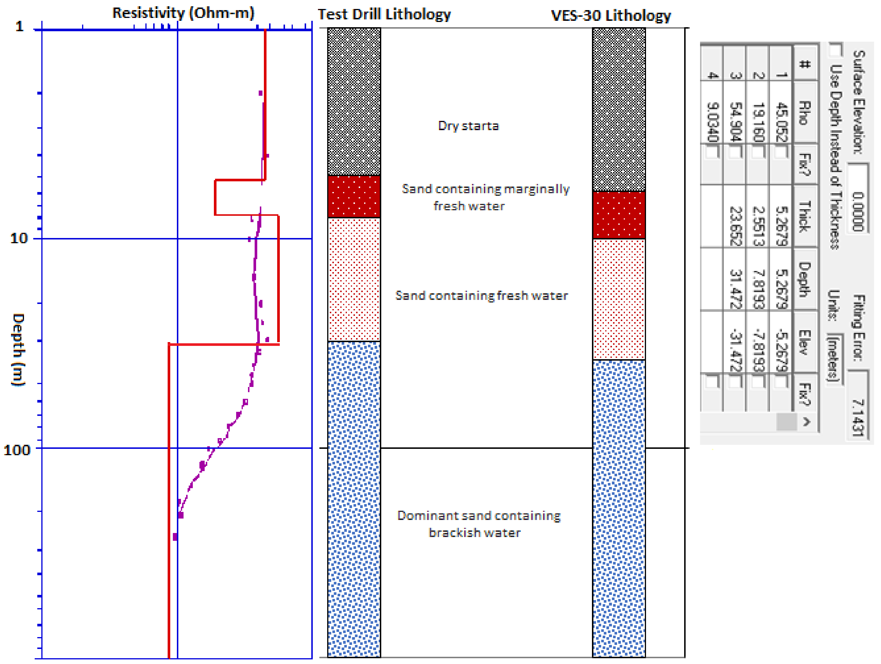
| Resistivity (ohm-m) | Lithology |
|---|---|
| Less than 20 | Silt containing saline water; Dominant sand containing brackish water |
| 20–40 | Sand containing marginally fresh water |
| 40–55 | Sand containing fresh water |
| Greater than 55 | Mixture of sand and minor gravel containing fresh water |
| Polygon # | Log Kpump (m/s) | Log Klab (m/s) | Kdiff = Log Kpump−Log Klab (m/s) | Test Hole Klab (m/s) | Log Klab (m/s) | Log Kmodel =Kdiff + Log Klab (m/s) | Kmodel (m/s) | Geometric Mean K (m/day) |
|---|---|---|---|---|---|---|---|---|
| 1 | −2.5430 | −5.2940 | 2.7510 | 3.20 × 10 −7 | -6.49 | −3.74 | 1.80 × 10⁻⁴ | 12.11 |
| 3.84 × 10 −7 | -6.42 | −3.66 | 2.16 × 10⁻⁴ | |||||
| 2.90 × 10 −7 | −6.54 | −3.79 | 1.63 × 10⁻⁴ | |||||
| 1.77 × 10 −8 | −7.75 | −5.00 | 1.00 × 10⁻⁵ | |||||
| 1.49 × 10 −7 | −6.83 | −4.07 | 8.41 × 10⁻⁵ | |||||
| 8.41 × 10 −7 | −6.08 | −3.32 | 4.75 × 10⁻⁴ | |||||
| 1.83 × 10 −7 | −6.74 | −3.99 | 1.03 × 10⁻⁴ | |||||
| 1.01 × 10 −6 | −6.00 | −3.25 | 5.67 × 10⁻⁴ | |||||
| 2 | −3.0160 | −5.4610 | 2.4450 | 7.68 × 10 −7 | −6.11 | −3.67 | 2.14 × 10⁻⁴ | 23.67 |
| 1.77 × 10 −6 | −5.75 | −3.31 | 4.94 × 10⁻⁴ | |||||
| 9.97 × 10 −7 | −6.00 | −3.56 | 2.78 × 10⁻⁴ | |||||
| 3.78 × 10 −6 | −5.42 | −2.98 | 1.05 × 10⁻³ | |||||
| 1.80 × 10 −7 | −6.75 | −4.30 | 5.00 × 10⁻⁵ | |||||
| 3 | −2.3450 | −4.7720 | 2.4270 | 2.41 × 10 −7 | −6.62 | −4.19 | 6.43 × 10⁻⁵ | 4.35 |
| 4.39 × 10 −7 | −6.36 | −3.93 | 1.17 × 10⁻⁴ | |||||
| 1.10 × 10 −7 | −6.96 | −4.53 | 2.95 × 10⁻⁵ | |||||
| 3.05 × 10 −8 | −7.52 | −5.09 | 8.14 × 10⁻⁶ | |||||
| 8.47 × 10 −7 | −6.07 | −3.64 | 2.26 × 10⁻⁴ | |||||
| 5.36 × 10 −7 | −6.27 | −3.84 | 1.43 × 10⁻⁴ | |||||
| 5.18 × 10 −8 | −2.06 | −1.32 | 1.38 × 10⁻⁵ | |||||
| 4 | −2.9064 | −5.4000 | 2.4936 | 3.84 × 10 −7 | −6.42 | −3.92 | 1.20 × 10⁻⁴ | 20.73 |
| 5.09 × 10 −7 | −6.29 | −3.80 | 1.58 × 10⁻⁴ | |||||
| 1.02 × 10 −6 | −5.99 | −3.50 | 3.20 × 10⁻⁴ | |||||
| 4.45 × 10 −7 | −6.35 | −3.86 | 1.39 × 10⁻⁴ | |||||
| 7.77 × 10 −7 | −6.11 | −3.62 | 2.43 × 10⁻⁴ | |||||
| 3.02 × 10 −6 | −5.52 | −3.03 | 9.42 × 10⁻⁴ | |||||
| 7.62 × 10 −7 | −6.12 | −3.62 | 2.38 × 10⁻⁴ | |||||
| 5 | −2.8090 | −5.3650 | 2.5560 | 1.74 × 10 −7 | −6.76 | −4.20 | 6.25 × 10⁻⁵ | 19.83 |
| 1.16 × 10 −6 | −5.94 | −3.38 | 4.18 × 10⁻⁴ | |||||
| 1.87 × 10 −7 | −6.73 | −4.17 | 6.74 × 10⁻⁵ | |||||
| 2.78 × 10 −6 | −5.56 | −3.00 | 1.00 × 10⁻³ | |||||
| 1.01 × 10 −6 | −6.00 | −3.44 | 3.63 × 10⁻⁴ | |||||
| 6 | −2.6190 | −5.4030 | 2.7840 | 6.10 × 10 −7 | −6.21 | −3.43 | 3.72 × 10⁻⁴ | 16.85 |
| 1.71 × 10 −7 | −6.77 | −3.98 | 1.04 × 10⁻⁴ | |||||
| 3.17 × 10 −7 | −6.50 | −3.71 | 1.93 × 10⁻⁴ | |||||
| 7 | −2.4300 | −5.5850 | 3.1550 | 7.62 × 10 −8 | −7.12 | −3.96 | 1.09 × 10⁻⁴ | 41.35 |
| 4.57 × 10 −7 | −6.34 | −3.18 | 6.55 × 10⁻⁴ | |||||
| 4.27 × 10 −7 | −6.37 | −3.21 | 6.10 × 10⁻⁴ | |||||
| 8.47 × 10 −7 | −6.07 | −2.92 | 1.21 × 10⁻³ | |||||
| 8 | −2.4990 | −4.9720 | 2.4730 | 3.29 × 10 −7 | −6.48 | −4.01 | 9.78 × 10⁻⁵ | 10.74 |
| 4.30 × 10 −7 | −6.37 | −3.89 | 1.28 × 10⁻⁴ | |||||
| 5.18 × 10 −7 | −6.29 | −3.81 | 1.54 × 10⁻⁴ | |||||
| 9 | −2.7310 | −5.5470 | 2.8160 | 2.13 × 10 −7 | −6.67 | −3.85 | 1.40 × 10⁻⁴ | 7.90 |
| 9.14 × 10 −8 | −7.04 | −4.22 | 5.97 × 10⁻⁵ | |||||
| 10 | −2.6600 | −5.2430 | 2.5830 | 2.13 × 10 −7 | −6.67 | −4.09 | 8.17 × 10⁻⁵ | 22.75 |
| 1.39 × 10 −6 | −5.86 | −3.27 | 5.33 × 10⁻⁴ | |||||
| 4.54 × 10 −7 | −6.34 | −3.76 | 1.74 × 10⁻⁴ | |||||
| 2.14 × 10 −6 | −5.67 | −3.09 | 8.17 × 10⁻⁴ | |||||
| 5.36 × 10 −7 | −6.27 | −3.69 | 2.05 × 10⁻⁴ | |||||
| 11 | −2.9010 | −5.5050 | 2.6040 | 9.14 × 10 −8 | −7.04 | −4.43 | 3.66 × 10⁻⁵ | 6.14 |
| 3.05 × 10 −8 | −7.52 | −4.91 | 1.23 × 10⁻⁵ | |||||
| 3.81 × 10 −7 | −6.42 | −3.82 | 1.53 × 10⁻⁴ | |||||
| 9.45 × 10 −7 | −6.02 | −3.42 | 3.81 × 10⁻⁴ | |||||
| 1.74 × 10 −7 | −6.76 | −4.16 | 6.98 × 10⁻⁵ | |||||
| 12 | −2.9930 | −5.6510 | 2.6580 | 2.33 × 10 −6 | −5.63 | −2.97 | 1.06 × 10⁻³ | 40.56 |
| 4.57 × 10 −7 | −6.34 | −3.68 | 2.08 × 10⁻⁴ | |||||
| 13 | −2.7770 | −5.4480 | 2.6710 | 2.34 × 10 −6 | −5.63 | −2.96 | 1.10 × 10⁻³ | 34.24 |
| 7.01 × 10 −7 | −6.15 | −3.48 | 3.29 × 10⁻⁴ | |||||
| 2.86 × 10 −7 | −6.54 | −3.87 | 1.34 × 10⁻⁴ | |||||
| 5.64 × 10 −6 | −5.25 | −2.58 | 2.64 × 10⁻³ | |||||
| 1.65 × 10 −7 | −6.78 | −4.11 | 7.71 × 10⁻⁵ | |||||
| 14 | −2.9000 | −5.3100 | 2.4100 | 6.10 × 10 −7 | −6.21 | −3.80 | 1.57 × 10⁻⁴ | 39.24 |
| 5.15 × 10 −6 | −5.29 | −2.88 | 1.32 × 10⁻³ | |||||
| 15 | −1.8210 | −6.0140 | 4.1930 | 3.05 × 10 −8 | −7.52 | −3.32 | 4.75 × 10⁻⁴ | 65.05 |
| 7.62 × 10 −8 | −7.12 | −2.93 | 1.19 × 10⁻³ | |||||
| 16 | −2.4260 | −6.1510 | 3.7250 | 3.05 × 10 −8 | −7.52 | −3.79 | 1.62 × 10⁻⁴ | 85.59 |
| 3.90 × 10 −6 | −5.41 | −1.68 | 2.07 × 10⁻² | |||||
| 1.34 × 10 −7 | −6.87 | −3.15 | 7.13 × 10⁻⁴ | |||||
| 7.62 × 10 −8 | −7.12 | −3.39 | 4.05 × 10⁻⁴ | |||||
| 17 | −2.9180 | −5.3760 | 2.4580 | 5.97 × 10 −7 | −6.22 | −3.77 | 1.71 × 10⁻⁴ | 14.80 |
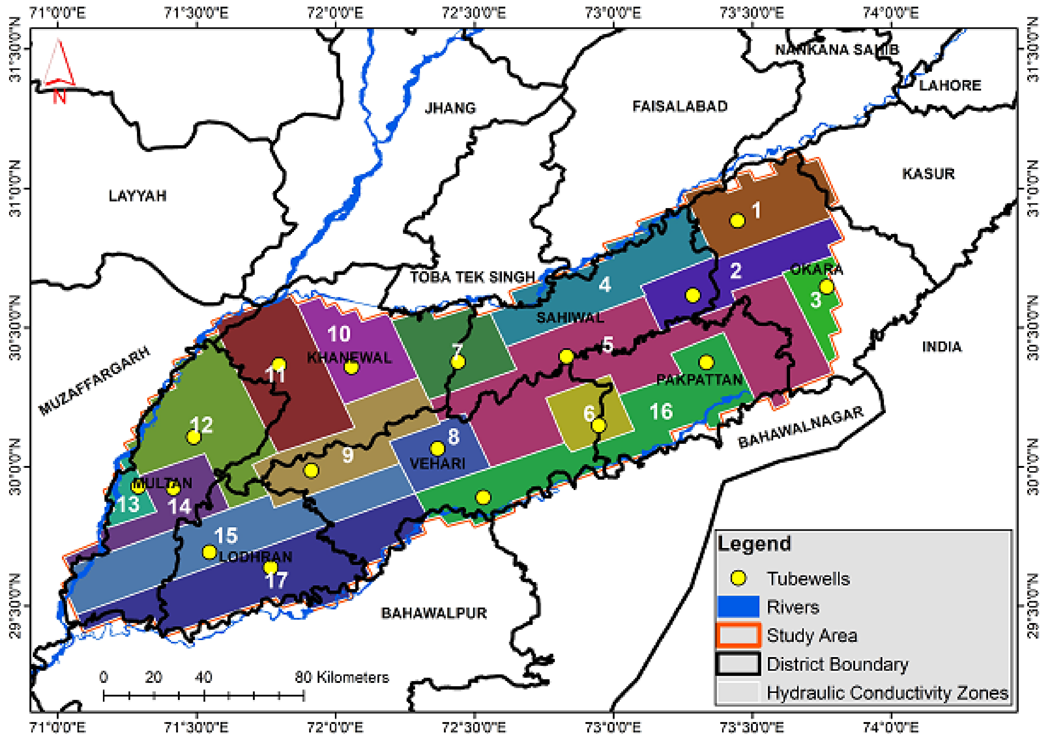
| Polygon# | K (m/Day) | Φ (%) | Formation Factor (F) | Aquifer Resistivity (Ohm-m) | Aquifer Thickness (m) | Tortuosity | Transmissivity m2/Day |
|---|---|---|---|---|---|---|---|
| 1 | 12.11 | 36.72 | 6.71 | 28–52 | 78 | 15.7 | 944.89 |
| 2 | 23.67 | 39.74 | 5.77 | 26–48 | 57 | 15.1 | 1349.47 |
| 3 | 4.35 | 32.11 | 12.17 | 32–55 | 155 | 19.8 | 673.51 |
| 4 | 20.73 | 39.14 | 4.49 | 29–63 | 64 | 13.2 | 1326.43 |
| 5 | 19.83 | 38.94 | 4.52 | 34–69 | 105 | 13.3 | 2082.15 |
| 6 | 16.85 | 38.21 | 5.65 | 35–82 | 164 | 14.7 | 2764.09 |
| 7 | 41.35 | 42.25 | 5.14 | 31–69 | 139 | 14.7 | 5747.03 |
| 8 | 10.74 | 36.18 | 6.90 | 21–67 | 176 | 15.8 | 1891.04 |
| 9 | 7.90 | 34.80 | 7.43 | 26–71 | 172 | 16.1 | 1358.87 |
| 10 | 22.75 | 39.56 | 8.44 | 22–81 | 85 | 18.3 | 1934.02 |
| 11 | 6.14 | 33.66 | 12.23 | 29–88 | 178 | 20.3 | 1092.21 |
| 12 | 40.56 | 42.16 | 7.29 | 32–69 | 170 | 17.5 | 6894.43 |
| 13 | 34.24 | 41.40 | 7.60 | 25–66 | 167 | 17.7 | 5717.27 |
| 14 | 39.24 | 42.01 | 4.00 | 23–51 | 175 | 13.0 | 6866.78 |
| 15 | 65.05 | 44.29 | 4.70 | 28–48 | 101 | 14.4 | 6569.72 |
| 16 | 85.59 | 45.52 | 4.46 | 32–54 | 105 | 14.2 | 8986.72 |
| 17 | 14.80 | 37.63 | 8.59 | 33–64 | 183 | 18.0 | 2708.42 |
Publisher’s Note: MDPI stays neutral with regard to jurisdictional claims in published maps and institutional affiliations. |
© 2022 by the authors. Licensee MDPI, Basel, Switzerland. This article is an open access article distributed under the terms and conditions of the Creative Commons Attribution (CC BY) license (https://creativecommons.org/licenses/by/4.0/).
Share and Cite
Akhter, G.; Ge, Y.; Hasan, M.; Shang, Y. Estimation of Hydrogeological Parameters by Using Pumping, Laboratory Data, Surface Resistivity and Thiessen Technique in Lower Bari Doab (Indus Basin), Pakistan. Appl. Sci. 2022, 12, 3055. https://doi.org/10.3390/app12063055
Akhter G, Ge Y, Hasan M, Shang Y. Estimation of Hydrogeological Parameters by Using Pumping, Laboratory Data, Surface Resistivity and Thiessen Technique in Lower Bari Doab (Indus Basin), Pakistan. Applied Sciences. 2022; 12(6):3055. https://doi.org/10.3390/app12063055
Chicago/Turabian StyleAkhter, Gulraiz, Yonggang Ge, Muhammad Hasan, and Yanjun Shang. 2022. "Estimation of Hydrogeological Parameters by Using Pumping, Laboratory Data, Surface Resistivity and Thiessen Technique in Lower Bari Doab (Indus Basin), Pakistan" Applied Sciences 12, no. 6: 3055. https://doi.org/10.3390/app12063055
APA StyleAkhter, G., Ge, Y., Hasan, M., & Shang, Y. (2022). Estimation of Hydrogeological Parameters by Using Pumping, Laboratory Data, Surface Resistivity and Thiessen Technique in Lower Bari Doab (Indus Basin), Pakistan. Applied Sciences, 12(6), 3055. https://doi.org/10.3390/app12063055