Application of Spearman’s Method for the Analysis of the Causes of Long-Term Post-Failure Downtime of City Buses

Abstract

The aim of this study was to analyze the impact of the categories of bus downtime caused by the necessity of their repair on the availability indicator. A retrospective study covering 12 years of bus operation was carried using the selected municipal transport company as an example. The share of the selected categories of downtime in the total time of vehicle downtime was analyzed. The Spearman’s rank correlation coefficient was used for the analysis. The research covered seven makes and types of buses and six categories of downtime. A ranking of the downtime categories was developed according to the criterion of the statistical dispersion of stoppage time as a measure of their unpredictability. It was shown that categorized unavailability was strongly dependent on the rank of downtime and loosely dependent on the age of buses. In practical applications, the test results may be useful in improving the fleet maintenance processes, selecting the make of new buses or development of models for safety margin availability.

1. Introduction

The availability of the transport system in general depends on the reliability and serviceability of vehicles and the conditions of their use, as well as the quality of the technical service [1,2,3].

AT = f (R_v, M_v, K, O_ZM)

(1)

where AT—vehicle availability, R_v—vehicle reliability, M_v—vehicle serviceability, K—operating conditions, O_ZM—quality of technical services and repairs.

The concept of availability is often used in rapid response systems when the moments of launching operational tasks are sudden (unplanned), e.g., in the air force, ambulance services or the fire brigade [4,5,6,7,8]. In recent years, the concept of using the availability criterion has gained wide recognition also in the management of public transport companies. In general, companies want to reduce costs while guaranteeing business continuity. According to Formula (1), an increase in the availability of the transport system can be ensured by:

• using vehicles with higher reliability;
• maintaining proper standards of operation;
• improving organizational procedures and staff competences as well as technology of technical maintenance and repairs of the vehicle fleet.

The analysis of methods to improve the availability of transport systems has been the subject of many scientific studies. The paper [9] presents various methods of estimating the relationship between the quality of transport services and selected quality factors, including the availability of the transport service, effectiveness of the offer information, the timeliness of the services, and customer service standards.

In the works [10,11], the problem of the relationship between the vehicle availability and maintenance costs was analyzed. The model of optimal inspections and technical service strategy, from the point of view of costs, was presented. Knowing the costs of operation, the operator can control those costs, and thus financial risk decreases, connected with planned and preventive as well as forced maintenance of vehicles, significantly limiting the risk of fleet availability and decreasing the risk related to safety of transport activities [12,13]. The papers [14,15] conducted analyses on the impact of bus reliability and the shift system of service operation on increasing the availability and reducing the costs of maintaining the transport system. The works [16,17] present a model of urban transport enterprise management, taking into account the design of travel routes and the selection of transport means and timetables. In the papers [18,19], the authors proposed the use of the semi-Markov model in relation to the selected example of public bus transport. The work [20] presents a method of continuous identification of the technical condition of city bus engines as the basis for optimizing the maintenance process.

The papers [21,22,23,24] describe the use of the availability index to improve city bus timetables and to monitor and maintain the punctuality of trips. The method of increasing the availability of the transport system by improving the efficiency of the repair subsystem is described by [25]. A queuing model with delayed repair and two maintenance phases was proposed. On the basis of this, the size of the queue of the vehicles waiting for repair was optimized. In the conclusion, it was emphasized that rationalizing the organization of the service process creates, in the long run, great opportunities to minimize the costs of maintaining high fleet availability.

Guided by those assumptions, we undertook a study of the availability of buses during 12 years of their operation at a selected municipal transport company. The observations covered the operation process of 162 buses of 7 makes and model. The objective of the research was to analyze the relationship between availability and the category (type) of bus downtime and the time of their operation. This article is an extension of the previous studies presented by the authors in the papers [26,27,28,29].

2. Research Method

2.1. Availability Indicator

The availability of the vehicle is defined as the probability that the vehicle is capable of performing the required function under given conditions at a given moment in time. The state of unavailability of the object means that the vehicle is unable to work due to technical malfunctions or due to organizational errors, e.g., related to the provision of necessary external resources, including spare parts and warranty services [23]. System availability is defined similarly in relation to the fleet of vehicles cooperating in the system.

The model of the vehicle operation process can be treated as a sequence of successive states of availability and unavailability [7]. A simple two-state model of the vehicle operation was chosen. The formula for AT availability indicator [30,31] can be written as

$$AT=\frac{{{\displaystyle \sum }}_{i=1}^{n}A{T}_i}{{{\displaystyle \sum }}_{i=1}^{n}A{T}_i+{{\displaystyle \sum }}_{i=1}^{n}U{T}_i}\ast 100\%$$

(2)

where AT_i—availability time of the tested sample of objects (vehicles) in the i-th observation interval (Availability Time); i = 1, 2, 3, …, n—number of the considered observation interval (month).

In this study, AT_i availability time was measured by the number of active vehicle-days defined as the product of the number of working days in the considered month of observation and the total number of vehicles conducting transport activities and operational vehicles remaining in reserve.

UT_i—unavailability time of the tested sample of objects (vehicles) in the i-th observation interval.

The sum written in the denominator, found in Formula (2), is the total inventory time T_c of the tested vehicle sample expressed in vehicle-days.

$$T_c={\displaystyle \sum }_{i=1}^{n}A{T}_i+{\displaystyle \sum }_{i=1}^{n}U{T}_i{}_{}$$

(3)

Adequately alongside Formula (2), the UT unavailability indicator can be represented by the following formula:

$$UT=\frac{{{\displaystyle \sum }}_{i=1}^{n}U{T}_i}{{{\displaystyle \sum }}_{i=1}^{n}A{T}_i+{{\displaystyle \sum }}_{i=1}^{n}U{T}_i}\ast 100\%$$

(4)

2.2. Downtime Categorization and Categorized Unavailability Coefficient

In this paper, the division of vehicle downtime caused by maintenance or repair for 6 categories was adopted, depending on the reasons for their unavailability. This division is used in practice in the examined enterprise. The following categories of downtime were taken into account.

• NB—current repair;
• ON—awaiting repair by an external service (mainly for warranty repairs);
• BCZ—awaiting spare parts;
• NW—post-accident repair;
• WS—engine replacement;
• INN—downtime due to other reasons not mentioned above.

In accordance with the adopted categorization of downtime, the concept of “categorized unavailability” of the vehicle was introduced. It was defined as the operational state of non-availability (standstill) corresponding to the downtime of a specific category. As an indicator of the quantitative assessment of the impact of a given category of downtime on the availability of buses, the “categorized unavailability coefficient” of the UT_k, is defined by the following formula:

$$U{T}_k=\frac{{{\displaystyle \sum }}_{i=1}^{n}U{T}_{ik}}{{{\displaystyle \sum }}_{i=1}^{n}U{T}_i}\ast 100\%$$

(5)

where UT_ik—the downtime of the tested sample of vehicles in the i-th observation interval due to the k-category downtime (Unavailability Time) expressed in vehicle-days.

The UT_k coefficient was interpreted as an indicator of the frequency of a given downtime category in the total downtime period in the i-th interval.

2.3. Spearman’s Rank Correlation Coefficient

In this paper, the Spearman rank correlation coefficient was used to study the impact of the vehicle downtime category and their age on availability. This coefficient is used for the non-parametric analysis of the relationship between two variables.

The rank correlation coefficient assumes a value in the range [−1; 1]. The closer the value of this measure is to −1, the stronger the negative correlation between the examined features, while the closer it is to +1, the stronger the positive correlation. Values close to zero indicate a weak relationship between the variables.

$$R_s=1-\frac{6{{\displaystyle \sum }}_{i=1}^N{d}_i^2{}_{}}{N\left(N^{2 }-1\right)}$$

(6)

where d_i—differences between the ranks of the corresponding values of x_i and y_i, i.e., the ranks of the X and Y features for individual research units.

In line with the objective of the research in this paper, the variable X represents the category of downtime k, and the variable Y is the coefficient of categorized unavailability UT_k determined by Formula (5). In the second stage of the analysis, the vehicle’s operating time (vehicle’s age) was assumed as the X variable, and the system availability and categorized unavailability coefficient as the Y variable.

In ranking of the bus stoppage category, it was assumed that the decisive feature of the downtime gradation is the proportion of the influence of random factors to the deterministic factors. It was taken into account that the influence of random factors (causes) on the duration of the downtime reduces its predictability and thus limits the possibility of managing the vehicle repair process. The V(UT_k) variation coefficient was assumed as the criterion for ranking downtime calculated according to the following formula:

$$V\left(U{T}_k\right)=\frac{SD(U{T}_k)}{M\left(U{T}_k\right)}$$

(7)

where M(UT_k) is the mean value of the U_k variable, and SD(UT_k) is the standard deviation of the UT_k variable.

3. The Course of Research

The experimental research was carried out at the Municipal Transport Company in Lublin using the retrospective method. The observations covered the operation process of 162 buses of 7 makes and models over a period of 12 years (2008–2019). The characteristics of the tested bus sample is shown in

Table 1. Characteristics of the studied bus sample during 12 years of operation.

No.	Vehicle’s Make	Manufacturer’s Prestige	Name of the Indicator
			Length of the Vehicle (m)	Number of the Vehicles Tested (pcs)	Average Daily Mileage of the Vehicle (km)
1	A	Low	12	53	201.3
2	B	Low	9	20	151.3
3	C	High	18	27	171.5
4	D	High	9	10	221.8
5	E	High	18	10	217.6
6	F	High	12	22	225.7
7	G	Medium	12	20	226.0

. The table shows the conventionally adopted estimate of the manufacturer’s prestige, considered in this study as an indicator of the expected quality of vehicles. The day and time of departure and return of vehicles to the depot as well as that of the downtime while under repair were recorded. The source documentation was the daily reports of the company. Data on the completed transports and vehicles’ downtime were arranged according to the monthly intervals.

The tested buses served regular public transport routes. The average daily mileages were about 202 km. The lowest average daily mileage was recorded for the B make bus—151.3 km. The highest daily mileage was recorded for the buses F and G—225.7 km and 226 km, respectively.

4. The Research Results

The data on bus downtime in monthly intervals were arranged according to the downtime categories (reasons for unavailability) of vehicles. Using Formula (2), the AT availability factor of each make of vehicles was calculated in the entire observed period of operation (144 months). Using Formula (4), the UT_k categorized unavailability rate was calculated for the following categories: NB, ON, BCZ, NW, WS, and NN.

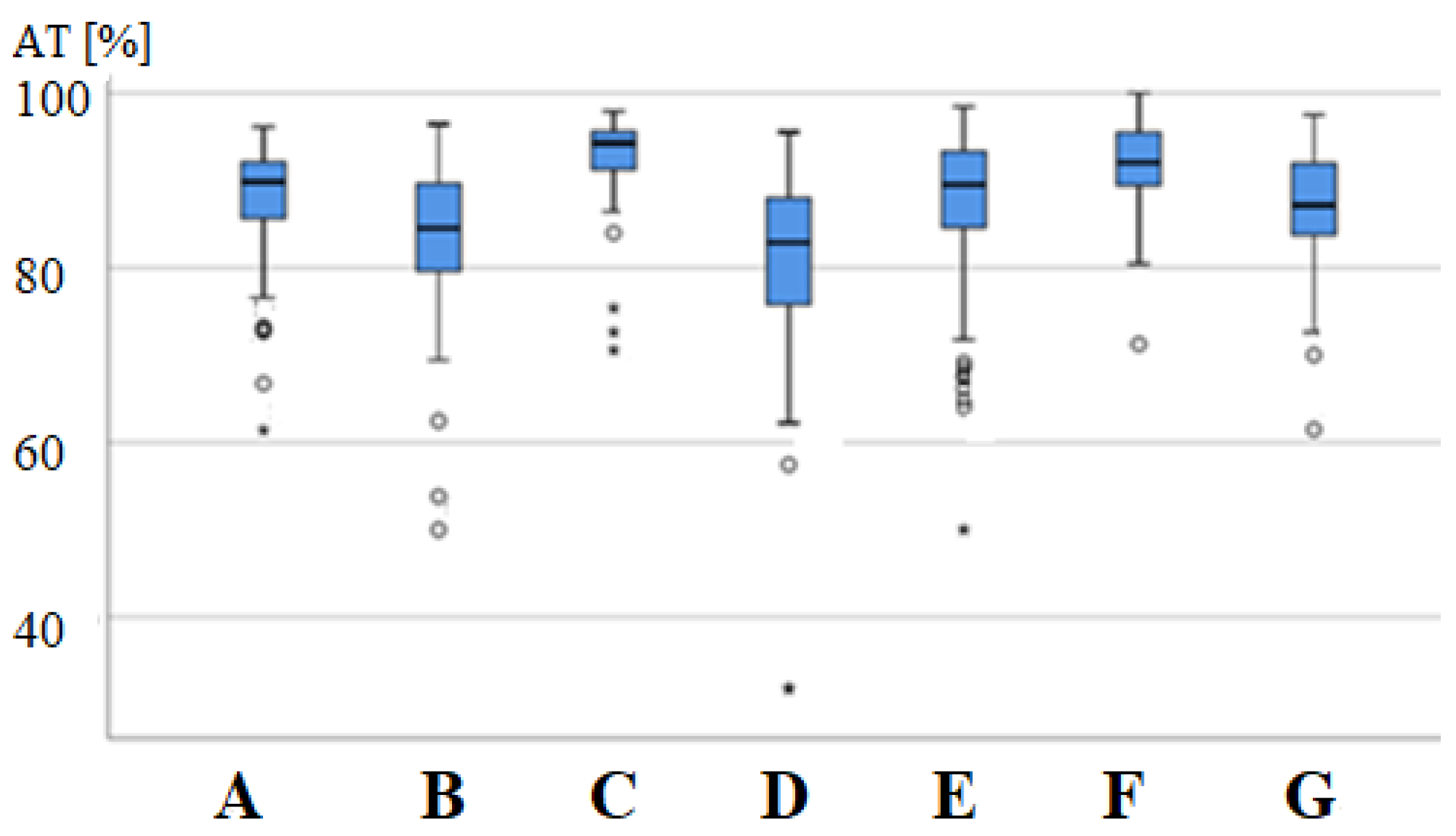
4.1. Descriptive Statistics of AT Availability and UT’s Categorized Unavailability

Using the IBM SPSS Statistics 25 package, a statistical analysis of the AT availability coefficients distribution and the categorized UT_k unavailability coefficient was performed. In particular, the descriptive statistics were determined: mean value, median, standard deviation, coefficient of variation, maximum and minimum value. The obtained values of the statistics concerning the availability ratio are presented in

Table 2. Descriptive statistics for the buses’ AT availability indicators.

No.	Vehicle’s Make	Number of Vehicles (pcs)	M(AT) (%)	Me(AT) (%)	SD(AT) (%)	V(AT)	Min. (%)	Max. (%)
1	A	53	88.07	89.84	6.36	0.07	61.39	96.13
2	B	20	83.49	84.50	8.62	0.10	50.00	96.45
3	C	27	92.73	94.27	4.88	0.05	70.55	97.90
4	D	10	81.03	82.89	9.92	0.12	31.82	95.53
5	E	10	87.97	89.50	7.71	0.09	50.00	98.41
6	F	22	91.55	92.05	5.41	0.06	71.24	100.00
7	G	20	87.18	87.16	6.07	0.07	61.48	97.50

M(AT)—mean availability; Me(AT)—median of the availability; SD(AT)—standard deviation; V(AT)—variation coefficient; Min and Max—minimum and maximum value.

. The frame chart of the AT availability indicator is presented in Figure 1. A summary of the descriptive statistics for the categorized unavailability coefficient is presented in

Table 3. Descriptive statistics of the categorized UT_k availability and the result of the Shapiro–Wilk test.

Vehicle’s Make	Downtime Category	M(UTk) (%)	Me(UTk) (%)	SD(UTk) (%)	V(UTk)	Min. (%)	Max. (%)	W	p
A	NB	39.41	36.26	16.29	0.41	14.39	95.50	0.94	<0.001
	ON	10.09	7.27	10.76	1.07	0.00	43.74	0.86	<0.001
	BCZ	17.19	14.31	14.26	0.83	0.00	59.71	0.93	<0.001
	NW	14.60	11.90	11.53	0.79	0.00	55.56	0.93	<0.001
	WS	1.93	0.00	5.33	2.76	0.00	23.67	0.41	<0.001
	INN	11.54	5.11	15.60	1.35	0.00	64.44	0.75	<0.001
B	NB	44.88	40.38	25.90	0.58	3.76	95.08	0.95	0.007
	ON	8.15	3.49	13.45	1.65	0.00	57.61	0.65	<0.001
	BCZ	14.36	8.59	16.29	1.13	0.00	74.07	0.83	<0.001
	NW	6.51	2.67	8.52	1.31	0.00	35.20	0.77	<0.001
	WS	-	-	-	-	-	-	-	-
	INN	21.78	5.32	24.43	1.12	0.00	75.84	0.82	<0.001
C	NB	45.79	41.38	21.31	0.46	7.32	91.43	0.96	0.005
	ON	9.49	2.46	13.88	1.46	0.00	52.75	0.72	<0.001
	BCZ	14.03	6.06	17.08	1.22	0.00	66.67	0.81	<0.001
	NW	14.44	9.52	16.88	1.17	0.00	67.57	0.81	<0.001
	WS	-	-	-	-	-	-	-	-
	INN	8.24	0.00	16.64	2.02	0.00	70.00	0.55	<0.001
D	NB	63.11	64.76	17.93	0.28	17.02	97.92	0.98	0.080
	ON	7.60	2.84	10.04	1.32	0.00	46.43	0.78	<0.001
	BCZ	12.80	7.44	14.16	1.11	0.00	55.22	0.84	<0.001
	NW	4.64	0.86	7.10	1.53	0.00	34.65	0.71	<0.001
	WS	1.12	0.00	4.65	4.15	0.00	41.10	0.26	<0.001
	INN	5.56	0.78	12.27	2.20	0.00	73.86	0.51	<0.001
E	NB	56.22	57.14	22.30	0.40	8.77	100.00	0.98	0.049
	ON	7.88	2.00	12.21	1.55	0.00	53.73	0.70	<0.001
	BCZ	19.97	15.59	19.16	0.96	0.00	80.85	0.89	<0.001
	NW	6.88	0.00	11.92	1.73	0.00	65.09	0.65	<0.001
	WS	0.26	0.00	2.44	9.38	0.00	23.62	0.08	<0.001
	INN	3.57	0.00	9.27	2.6	0.00	60.00	0.44	<0.001
F	NB	53.23	53.64	21.97	0.41	14.29	100.00	0.96	0.110
	ON	10.70	5.75	14.19	1.33	0.00	72.73	0.75	<0.001
	BCZ	16.87	9.25	17.77	1.05	0.00	61.70	0.85	<0.001
	NW	12.23	4.97	17.14	1.40	0.00	78.57	0.73	<0.001
	WS	-	-	-	-	-	-	-	-
	INN	6.96	1.22	15.35	2.20	0.00	85.71	0.51	<0.001
G	NB	51.24	50.00	20.10	0.39	13.79	100.00	0.98	0.024
	ON	8.93	4.27	12.15	1.36	0.00	55.81	0.75	<0.001
	BCZ	17.48	14.41	14.53	0.83	0.00	65.65	0.93	<0.001
	NW	9.31	3.70	12.82	1.38	0.00	80.00	0.74	<0.001
	WS	0.04	0.00	0.32	8.00	0.00	3.37	0.09	<0.001
	INN	10.00	3.85	13.49	1.35	0.00	68.00	0.75	<0.001

M(UT)—average; Me(UT)—median; SD(UT)—standard deviation; V(UT)—variation coefficient; Min and Max—the lowest and highest value of the distribution; W—Shapiro–Wilk test result; p—statistical significance of the S-W test.

. The results of the Shapiro–Wilk test concerning the assessment of the normality of the UT_k variable distribution are also given.

The results concerning the availability of buses presented in Figure 1 and in Table 2 show that the average availability over the total research period of 144 months was in the AT ≈ (81.03–92.73%) range depending on the make and model of the vehicle. The highest average availability was achieved by C and F makes, M(AT_C) vehicles = 92.73%; M(AT_F) = 91.55%). Both brands represented a manufacturer with high prestige. It is also worth noting that the coefficient of variation characterizing the uniqueness of the results had the lowest value here, V(AT_C) = 0.05 and V(AT_F) = 0.06. The lowest average availability was achieved by vehicles of makes D and B, M(AT_D) = 81.03% and M(AT_B) = 83.49%. In the literature, the availability of bus communication systems in large urban agglomerations in Poland at the level of 85–90% is assessed as good (satisfactory) in terms of smooth requirements for system (enterprise) functioning. Taking into account all makes and models of the tested buses, the average availability M(AT) = 87.43% was calculated. This result should be regarded as satisfactory from the point of view of the quality of the vehicle fleet and the effectiveness of the transport enterprise.

In the next stage of work, the share of particular categories of downtime in the total period of the vehicles’ unavailability of a given make was analyzed. Using Formula (4), the coefficient of unavailability of categorized UT_k was calculated, and then descriptive statistics of this coefficient were determined. The values of these statistics and the Shapiro–Wilk normality test result are given in Table 3. The result of the Shapiro–Wilk test for all the analyzed variables turned out to be statistically significant, which means that their distributions significantly differed from the normal distribution.

The results of the calculations indicate that the share of individual categories of downtime varied greatly. There was a large share of the NB category—“current repair”, M(UT_k) = 39.41% ÷ 63.11%. On the other hand, the smallest share in the total time of downtime was WS downtime—“engine replacement” within the range UT_k = 0.04 ÷ 2.0.

4.2. Selection of the Rank of Downtime Categories and Downtime Periods

In the next step of the analysis, the dependence of the amount of downtime categorized on downtime category was examined. The non-parametric Spearman method was used. The mean value M(UT_k) was adopted as the categorized stoppage value indicator, and the V(UT_k) coefficient was adopted as the stoppage category indicator according to Table 3. Taking into account the proportion between the influence of random and deterministic factors, the following ranking of the downtime category was developed:

• NB “current repair”—category NB includes repetitive maintenance procedures and repeated replacement of wearing parts; therefore, the influence of determined factors is of dominant character, while the influence of random factors is of minority character. In this study, the estimated V(NB) < 0.58 (Table 3).
• BCZ “lack of spare parts”—it is known from company practice that shortages of spare parts are events with a balanced influence of random and deterministic factors. In the study, it was estimated that V(BCZ) = 1.0 +/− 0.25 (Table 3).
• ON “pending repair”—downtime in this category is related to the awaiting warranty service by the manufacturer, and thus they mainly concern external causes and are difficult to predict and manage. It is known from practice that the influence of random factors (independent of the company’s management) is balanced here with the influence of deterministic factors. In the study, the estimated V(ON) = 1.25 +/− 0.25 (Table 3).
• NW “post-accident repair”—road accidents as the cause of vehicle downtime are random, but it is possible to predict repairs of this category on the basis of statistical data. In the presented research, it was estimated that V(NW) = 1.25 +/− 0.5 (Table 3).
• INN “other causes”—due to the large number and variety of non-standard causes of downtime, the role of the chance is very large here. In the study, the estimated V(INN) = 1.5 +/− 0.5 (Table 3).
• WS “engine replacement”—the WS category applies to defects that require removal of the engine, as a result of which the engine is replaced and the damaged vehicle is sent for repair in a separate cycle. It is known from company practice that there is a high uniqueness of downtime duration. In the study, the estimated V(WS) = 4.0 +/− 4.0 (Table 3).

On the basis of the data contained in Table 3, the V_k variation coefficient values characterizing individual categories of stoppages were compiled, the x_k ranks were adjusted, and the Spearman coefficient R_S was calculated. The compilation ranks for the downtime category and the results of the R_S Spearman coefficient calculations are provided in

Table 4. Downtime ranks and Spearman’s rank correlation coefficient between categorized unavailability and downtime category.

L	Downtime Category	x(NB)	x(BCZ)	x(ON)	x(NW)	x(INN)	x(WS)	Rs
	Bus Make
1	A	1	3	4	2	5	6	−0.88
2	C	1	3	5	4	5	6	−0.90
3	F	1	3	4	2	5	6	−1.00
4	B	1	2	3	4	5	6	−1.00
5	D	1	2	3	4	5	6	−1.00
6	E	1	2	3	4	5	6	−0.94
7	G	1	2	4	5	3	6	−0.61
xme		1	2.93	3.71	3.57	4.71	6	Rs.me = −0.90
Xest		1	2	4	3	5	6

Where X_est—estimated value of downtime rank; R_s.me—mean value of the Spearman coefficient.

.

The obtained result of Spearman’s coefficient calculation amounting to R_s.me = −0.90 (on average for all bus makes) indicates a negative strong relationship between the category and duration of downtime. In this paper, taking into account the adopted indicators, it means the relationship between the categorized unavailability coefficient (defined as the ratio of the number of coach days of unavailability caused by k-th cause to the total number of coach days of unavailability covering all causes) and the coefficient of statistical variability as a measure of variation in the tested sample of a given bus brand. The differences in the Spearman’s coefficient values between vehicle brands were significant. They were in the range from R_S(G) = −0.61 to R_S(E) = R_S(C) = R_S(D) = −1.00. In the case of low Rs, NB and WS downtimes of extreme ranks stood out. The other downtime categories were comparable in terms of the order of magnitude of the downtime. It concerns both UT_K = (10 ÷ 17)% and V_K = (0.83 ÷ 1.38).

In the next part of the empirical data analysis, the dependence of the coefficient of unavailability of categorized buses on their annual service life was checked. For this purpose, the Spearman correlation analysis was conducted, the results of which are presented in

Table 5. Spearman’s rank correlation coefficient between categorized unavailability and the age of the bus.

Vehicle Make	Downtime Categories
	∑—All Factors	NB—Current Repair	ON—Pending Repair	BCZ—No Spare Parts	NW—Accident Repair	WS—Engine Replacement	INN—Other
A	0.51	0.41	−0.65	0.09	0.01	0.46	−0.48
B	0.22	0.49	−0.40	0.36	−0.21		−0.59
C	0.11	0.30	−0.44	0.03	−0.1		−0.13
D	−0.07	0.05	0.17	−0.4	−0.11	0.36	−0.26
E	−0.12	−0.02	−0.22	0.09	−0.13	0.18	0.01
F	−0.19	0.21	0.11	0.07	0.22		0.13
G	−0.04	0.26	−0.25	0.13	−0.31		−0.40

.

The results of the Spearman’s rank correlation analysis showed for all the tested buses, except for the F model, that with the increase in vehicle usage time, the share of each category of downtime in the total vehicle downtime changed. For category NB—“current repairs”, the impact of operating time was positive. This applied to the following vehicles: make A (R = 0.41), make B (R = 0.49), make C (R = 0.30), and make G (R = 0.26). A similar relationship was observed in the case of the WS category—“engine replacement”. This applied to the following brands: A (R = 0.46), D (R = 0.36), and E (R = 0.18). For the ON category—“pending repair”, the impact of calendar time was negative. Spearman’s coefficients were A (R = −0.65), B (R = −0.40), C (R = −0.44), E (R = −0.22), and G (R = −0.25). A similar relationship occurred in the case of the INN category—“other”, wherein the Spearman coefficients were A (R = −0.48), B (R = −0.59), E (R = −0.13), D (R = −0.26), and G (R = −0.40). On the other hand, the BCZ category—“no spare parts” was correlated with the service life in a different way. This relationship was positive for B model vehicles (R = 0.36) and negative for D (R = −0.42).

5. Summary

On the basis of the conducted research, the following conclusions were drawn:

• The availability coefficient of buses of seven makes and models was determined for the 12 year period of their operation. The average availability value in the period under consideration was in the AT ≈ (81.03–92.7)% range, depending on the make and model of the bus. The highest average availability was achieved by C and F make vehicles—M(AT_c) vehicles = 92.7% and M(AT_F) = 91.5%. Both makes came from a high-profile manufacturer.
• A ranking of the downtime-type categories in the vehicle servicing system at the enterprise was created according to the criterion of downtime repeatability.
• The relationship between the category of downtime and the bus unavailability coefficient was determined as the basis for rationalization of bus fleet maintenance.
• It was shown that the share of categorized unavailability was strongly, negatively dependent on the category of downtime (Spearman’s rank coefficient R_s ≈ −(0.6 ÷ 1.0)) and mostly slightly positively dependent on the age of the buses (R_s ≈ (0.2 ÷ 0.4)).
• The largest share of the state of unavailability had downtime due to repetitive causes, and therefore for predictable reasons—NB (current repair). Unpredictable, difficult-to-manage downtimes were dictated by random WS—“engine replacement” and INN—”other” causes.

The availability of vehicles significantly affects the economy of transport services. With the increasing availability of vehicles, the unit’s fixed costs decrease. The growing availability of vehicles increases the competitiveness of the carrier.

References

1. Michalski, R.; Wierzbicki, S. Comparative reliability tests of city transport busses. Eksploat. Niezawodn.-Maint. Reliab. 2006, 4, 22–26. [Google Scholar]
2. Stapelberg, R.F. Handbook of Reliability, Availability, Maintainability and Safety in Engineering Design; Springer: London, UK, 2009. [Google Scholar]
3. Zio, E. Reliability engineering: Old problems and new challenges. Reliab. Eng. Syst. Saf. 2009, 94, 125–141. [Google Scholar] [CrossRef] [Green Version]
4. Herder, P.M.; van Luijk, J.A.; Bruijnooge, J. Industrial application of RAM modeling development and implementation of a RAM simulation model for the Lexan plant at GE Industrial. Reliab. Eng. Syst. Saf. 2008, 93, 501–508. [Google Scholar] [CrossRef]
5. Pham, H. Handbook of Reliability Engineering; Springer: London, UK, 2003. [Google Scholar]
6. Poliak, M.; Poliakova, A.; Svabova, L.; Zhuravleva, N.A.; Nica, E. Competitiveness of Price in International Road Freight Transport. J. Compet. 2021, 13, 83–98. [Google Scholar] [CrossRef]
7. Szkoda, M. Assessment of Reliability, Availability and Maintainability of Rail Gauge Change Systems. Eksploat. Niezawodn.-Maint. Reliab. 2014, 16, 422–432. [Google Scholar]
8. Jurecki, R.; Jaśkiewicz, M. Analysis of Road accidents over the last ten years. Zesz. Nauk. Akad. Mor. Szczecinie 2012, 32, 65–70. [Google Scholar]
9. Zhao, F.; Zeng, X. Optimization of transit route network, vehicle headways and timetables for large-scale transit networks. Eur. J. Oper. Res. 2008, 186, 841–855. [Google Scholar] [CrossRef]
10. Caban, J.; Droździel, P.; Krzywonos, L.; Rybicka, I.K.; Šarkan, B.; Vrábel, J. Statistical Analyses of Selected Maintenance Parameters of Vehicles of Road Transport Companies. Adv. Sci. Technol. Res. J. 2019, 13, 1–13. [Google Scholar] [CrossRef]
11. Xuan, Y.; Argote, J.; Daganzo, C.F. Dynamic bus holding strategies for schedule reliability: Optimal linear control and performance analysis. Transp. Res. Part B 2011, 45, 1831–1845. [Google Scholar] [CrossRef]
12. Andrzejczak, K.; Selech, J. Investigating the trends of average costs of corrective maintenance of public transport vehicles. J. KONBiN 2017, 41, 207–226. [Google Scholar] [CrossRef] [Green Version]
13. Jaśkiewicz, M.; Lisiecki, J.; Lisiecki, S.; Pokorski, E.; Więckowski, D. Facility for performance testing of power transmission units. Zesz. Nauk. Akad. Mor. Szczecinie. 2015, 42, 14–25. [Google Scholar]
14. Ruhang, X. Characteristics and prospective of China’s PV development route: Based on data of world PV industry 2000–2010. Renew. Sustain. Energy Rev. 2016, 56, 1032–1104. [Google Scholar] [CrossRef]
15. Savsar, M. Modeling and simulation of maintenance operations at Kuwait public transport company. Kuwait J. Sci. 2013, 40, 115–129. [Google Scholar]
16. Chen, X.; Xiao, L.; Zhang, X.; Xiao, W.; Li, J. An integrated model of production scheduling and maintenance planning under imperfect preventive maintenance. Eksploat. Niezawodn.-Maint. Reliab. 2015, 17, 70–79. [Google Scholar] [CrossRef]
17. Sanchez, S.A. Optimizing performance-based mechanisms in road management: An agency theory approach. Eur. J. Transp. Infrastruct. Res. 2015, 15, 465–481. [Google Scholar]
18. Borucka, A.; Niewczas, A.; Hasilova, K. Forecasting the readiness of special vehicles using the semi-Markov model. Eksploat. Niezawodn.-Maint. Reliab. 2019, 21, 662–669. [Google Scholar] [CrossRef]
19. Migawa, K. Semi-Markov model of the availability of the means of municipal transport system. Sci. Probl. Mach. Oper. Maint. 2009, 3, 25–34. [Google Scholar]
20. Grądzki, R.; Lindstedt, P. Method of assessment of technical object aptitude in environment of exploitation and service conditions. Eksploat. I Niezawodn.-Maint. Reliab. 2015, 17, 54–63. [Google Scholar] [CrossRef]
21. Guihaire, V.; Hao, J.K.H. Transit network design and scheduling: A global review. Transp. Res. Part A 2008, 42, 1251–1273. [Google Scholar] [CrossRef] [Green Version]
22. Guihaire, V.; Hao, J.K.H. Transit network timetabling and vehicle assignment for regulating authorities. Comput. Ind. Eng. 2010, 59, 16–23. [Google Scholar] [CrossRef] [Green Version]
23. Wolde, M.; Ghobbar, A.A. Optimizing inspection intervals—Reliability and availability in terms of a cost model: A case study on railway carriers. Reliab. Eng. Syst. Saf. 2013, 114, 137–147. [Google Scholar] [CrossRef]
24. Yatskiv, I.; Pticina, I.; Savrasovs, M. Urban public transport system’s reliability estimation using microscopic simulation. Transp. Telecommun. 2012, 13, 219–228. [Google Scholar] [CrossRef]
25. Choudhury, G.; Ke, J.C.; Tadj, L. The N-policy for an unreliable server with delaying repair and two phases of service. J. Comput. Appl. Math. 2009, 231, 349–364. [Google Scholar] [CrossRef] [Green Version]
26. Ignaciuk, P.; Rymarz, J.; Niewczas, A. Effectiveness of the failure rate on maintenance costs of the city buses. J. KONBiN 2015, 3, 99–108. [Google Scholar] [CrossRef] [Green Version]
27. Niewczas, A.; Rymarz, J.; Debicka, E. Stages of operating vehicles with respect to operational efficiency using city buses as an example. Eksploat. Niezawodn.-Maint. Reliab. 2019, 21, 21–27. [Google Scholar] [CrossRef]
28. Rymarz, J.; Niewczas, A.; Pieniak, D. Reliability analysis of the selected brands of city buses at municipal transport company. J. KONBiN 2013, 26, 111–122. [Google Scholar] [CrossRef] [Green Version]
29. Rymarz, J.; Niewczas, A.; Krzyżak, A. Comparison of operational availability of public city buses by analysis of variance. Eksploat. Niezawodn.-Maint. Reliab. 2016, 18, 373–378. [Google Scholar] [CrossRef]
30. Djeridi, R.; Cauvin, A. Operational availability assessment for improving the maintenance of the complex systems. In Proceedings of the 13th IFAC Symposium on Information Control Problems in Manufacturing, Moscow, Russia, 3–5 June 2009. [Google Scholar]
31. Djeridi, R.; Cauvin, A. Integration of a modelling method in the design of supply chains: Proposals of an approach in the framework of Design for Logistics. In Proceedings of the 5th International Conference JTEA’2008-IEEE, Hammamet, Tunisie, 2–4 May 2008. [Google Scholar]
Figure 1. Frame chart of the buses’ AT availability indicators.
Applsci 12 02921 g001