Abstract
In robust design (RD) modeling, the response surface methodology (RSM) based on the least-squares method (LSM) is a useful statistical tool for estimating functional relationships between input factors and their associated output responses. Neural network (NN)-based models provide an alternative means of executing input-output functions without the assumptions necessary with LSM-based RSM. However, current NN-based estimation methods do not always provide suitable response functions. Thus, there is room for improvement in the realm of RD modeling. In this study, a new NN-based RD modeling procedure is proposed to obtain the process mean and standard deviation response functions. Second, RD modeling methods based on the feed-forward back-propagation neural network (FFNN), cascade-forward back-propagation neural network (CFNN), and radial basis function network (RBFN) are proposed. Third, two simulation studies are conducted using a given true function to verify the proposed three methods. Fourth, a case study is examined to illustrate the potential of the proposed approach. In conclusion, a comparative analysis of the three feed-forward NN structure-based modeling methods and conventional LSM-based RSM proposed in this study showed that the proposed methods were significantly lower in the expected quality loss (EQL) and various variability indicators.
1. Introduction
In recent decades, robust design (RD) has been considered essential for improvement of product quality, as the primary purpose of RD is to seek a set of parameters that make a product insensitive to various sources of noise factors. In other words, RD attempts to minimize the variability of quality characteristics while ensuring that the process mean meets the target value. To solve the RD problem, Taguchi [1] considered both the process mean and variance as a single performance measure and defined a number of signal-to-noise ratios to obtain the optimal factor settings. Unfortunately, the orthogonal arrays (OAs), statistical analysis, and signal-to-noise ratios associated with this technique were criticized by Box et al. [2], Leon et al. [3], Box [4], and Nair [5]. Therefore, Vining and Myers [6] proposed the dual response (DR) approach based on response surface methodology (RSM), in which the process mean and variance are estimated separately as functions of control factors. The result is an RD optimization model in which the process mean is prioritized by setting it as a constraint and the process variability is set as an objective function. From this starting point, the three sequential steps of the RD procedure were generated: design of experiment (DoE), estimation, and optimization. The DoE step exploits information about the relationship between the input and output variables. In the second step, the functional form of this relationship is defined by estimating the model parameters. Ultimately, the optimal settings for the input factors are identified in the third step.
As several RD optimization models have been proposed and modified according to various criteria, the optimization step is relatively well developed. The priority criterion was used in the DR models proposed by Vining and Myers [6], Copeland and Nelson [7], and Del Castillo and Montgomery [8], whereas the process mean and variance were considered simultaneously in the mean squares error (MSE) model developed by Lin and Tu [9]. The weight criterion was used to consider the trade-off between the mean and variance in the weighted sum models reported by Cho et al. [10], Ding et al. [11], and Koksoy and Doganaksoy [12], whereas Ames et al. [13] used the weight criterion in a quality loss function model. Shin and Cho [14,15] extended the DR model by integrating the customized maximum value on the process bias and variance. Based on the MSE concept, Robinson et al. [16] and Truong and Shin [17] proposed generalized linear mixed models and inverse problem models. Using the goal programming approach, Kim and Cho [18] and Tang and Xu [19] introduced prioritized models, whereas Borror [20] and Fogliatto [21] both considered the output responses on the same scale as the desirability functions. In an attempt to identify the Pareto efficient solutions, Kim and Lin [22] and Shin and Cho [23] developed a fuzzy model and a lexicographical weighted Tchebycheff model for the RD multiple-objective optimization problem, respectively. Furthermore, Goethals and Cho [24] integrated the economic factor in the economic time-oriented model to handle time-oriented dynamic characteristics, while Nha et al. [25] introduced the lexicographical dynamic goal programming model.
The DoE is a systematic method that aims to identify the effects of controllable factors on the quality characteristics of interest. DOE has been developed since the 1920s. Montgomery [26] reviewed the history of DoE in the published literature. Several DoE techniques were developed and intensively researched as a means of conducting experiments in industrial applications; these include full factorial designs, fractional factorial designs (screening designs), mixture designs, Box-Benken designs, central composite designs (CCD), Taguchi array designs, Latin square designs and other non-conventional methods (D-optimal designs).
Although many techniques for the estimation stage of an RD process are reported in literature, there is room for improvement. Indeed, the accuracy and reliability of prediction and optimization depend directly on the estimation results. Additionally, most regression methods are RSM-based approaches which commonly rely on assumptions, such as normality and homogeneous variance of the response data. However, in practice, these assumptions may not be maintained.
Along with the development of RD, RSM has been widely applied in various fields of applied statistics. The most extensive applications of RSM are in the industrial world, particularly in situations where several input variables may influence some performance measure or quality characteristic of the product or process [27]. RSM uses mathematical and statistical techniques to explore the functional relationship between input control variables and an output response variable of interest, with the unknown coefficients in this functional relationship typically estimated by the least-squares method (LSM). The usual assumptions behind LSM-based RSM are that the experimental data and error terms must be normally distributed, and the distribution of error terms must have constant variance and zero mean. When one of these assumptions is violated, the Gauss-Markov theory no longer holds. Instead, alternative techniques can be applied, such as the maximum likelihood estimation (MLE), weighted least-squares (WLS), and Bayesian methods. From the viewpoint of MLE, the model parameters are regarded as fixed and unknown quantities, and the observed data are considered as random variables [28]. Truong and Shin [17,29] showed that LSM-based RSM does not always estimate the input-output functions effectively, so they developed a procedure to estimate these unknown coefficients using an inverse problem.
In recent decades, neural networks (NNs) have become a hot topic of research; NNs are now widely used in various fields, including speech recognition, multi-objective optimization, function estimation, and classification. NNs can model linear and nonlinear relationships between inputs and outputs without any assumptions based on the activation function’s generalization capacity. NNs are universal functional approximators, and Irie and Miyake [30], Funahashi [31], Cybenko [32] and Hornik et al. [33], and Zainuddin and Pauline [34] showed that NNs are capable of approximating any arbitrary nonlinear function to the desired accuracy without the knowledge of predetermined models, as NNs are data-driven and self-adaptive. Therefore, a NN provides a powerful regression method to model the functional relationship between RD input factors and output responses without making any assumptions. In RD settings, Rowlands et al. [35] integrated an NN into RD by using the NN to conduct the DoE stage. Su and Hsieh [36] applied two NNs to train the data to obtain the optimal parameter sets and predict the system response value. Cook et al. [37] developed an NN model to forecast a set of critical process parameters and employed a genetic algorithm to train the NN model to achieve the desired level of efficiency. The integration of NNs into RD has also been discussed by Chow et al. [38], Chang [39], and Chang and Chen [40]. Arungpadang and Kim [41] developed a feed-forward NN-based RSM to model the functional relationship between input variables and output responses to improve the precision of estimation without increasing the number of experimental runs. Sabouri et al. [42] proposed an NN-based method for function estimation and optimization by adjusting weights until the response reached the target conditions. With regard to input-output relationship modeling, Hong and Satriani [43] also discussed a convolutional neural network (CNN) with an architecture determined by Taguchi’s orthogonal array to predict renewable power. Recently, Arungpadang et al. [44] proposed a hybrid neural network-genetic algorithm to predict process parameters. Le et al. proposed NN-based response function estimation (NRFE) identifies a new screening procedure to obtain the best transfer function in an NN structure using a desirability function family while determining its associated weight parameters [45]. Le and Shin propose an NN-based estimation method as a RD modeling approach. The modeling method based on a feedback NN approach is first integrated in the RD response functions estimation. Two new feedback NN structures are then proposed. Next, the existing recurrent NNs (i.e., Jordan-type and Elman-type NNs) and the proposed feedback NN approaches are suggested as an alternative RD modeling method [46].
The primary motive of this research is to establish feed-forward NN structure-based estimation methods as alternative RD modeling approaches. First, an NN-based estimation framework is incorporated into the RD modeling procedure. Second, RD modeling methods based on the feed-forward back-propagation neural network (FFNN), cascade-forward back-propagation neural network (CFNN), and radial basis function network (RBFN) are proposed. These are applied to estimate the process mean and standard deviation response functions. Third, the efficiency of the proposed modeling methods is illustrated through simulation studies with a given real function. Fourth, the efficacy of the proposed modeling methods is illustrated through a printing case study. Finally, the results of comparative studies show that the proposed methods obtain better optimal solutions than conventional LSM-based RSM. The proposed estimation methods based on feed-forward NN structures are illustrated in Figure 1. From the experimental data, the optimal numbers of hidden neurons in the FFNN and CFNN structures and the dispersion constant “spread” in the RBFN are identified to finalize the optimal structures of the corresponding NNs. The DR functions can be separately estimated using the proposed estimation methods from the optimal NN structures with their control factors and output responses.
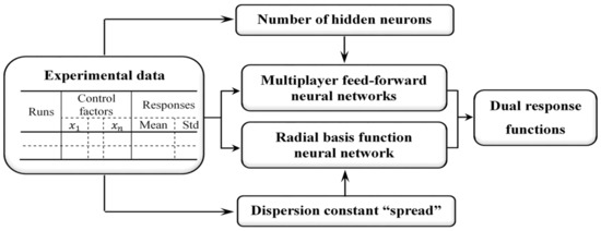
Figure 1.
Proposed NN-based estimation procedure.
The statistical estimation method of RSM based on conventional LSM, as introduced by Box and Wilson [47], generates the response surface approximation using linear, quadratic, and other functions, while the coefficients are estimated by minimizing the total error between the actual and estimated values. For a more comprehensive understanding of RSM, Myers [48] and Khuri and Mukhopadhyay [49] discuss the various development stages and future directions of RSM. When the exact functional relationship is unknown or very complicated, conventional LSM is typically used to estimate the input-output functional responses in RSM [50,51]. In general, the output response can be identified as a function of input factors as follows:
where is a vector of the control factors, is a column vector of the estimated parameters, and is the random error. The estimated second-order models for the process mean and standard deviation are represented as
where and are the estimators of unknown parameters in the mean and standard deviation functions, respectively. These coefficients are estimated using LSM as
where and are the average and standard deviation values for the experimental data, respectively.
2. Proposed Feed-Forward NN Structure-Based Estimation Methods
Abbreviations and main variables used in this study are summarized in Appendix D.
2.1. NN Structures
An artificial neuron is a computational model inspired by biological neurons [52]. A NN consists of numerous artificial neurons or nodes and the connections between them, with weight coefficients applied to each connection. Based on the pattern of connection, NNs typically fall into two distinct categories: feed-forward networks, in which the connection flows unidirectionally from input to output, and recurrent networks, in which the connections among layers run in both directions. Feed-forward networks are the most popular type for function approximation [34]. Therefore, this study uses feed-forward back-propagation networks and RBFN structures to estimate the desired functions.
2.2. Proposed NN-Based Estimation Method 1: FFNN Structure
2.2.1. Response Function Estimation Using FFNN
According to Taguchi’s philosophy, there are two output responses of interest, namely, the process mean and standard deviation. These output responses can be estimated simultaneously from the output layer in a single FFNN. Besides, as demonstrated by Cybenko [32], any continuous function of n input variables can be approximated by an FFNN with only one hidden layer. A similar notion is also discussed by Funahashi [31], Hornik et al. [33], and Hartman et al. [53]. The proposed FFNN-based RD modeling method with one hidden layer is illustrated in Figure 2.
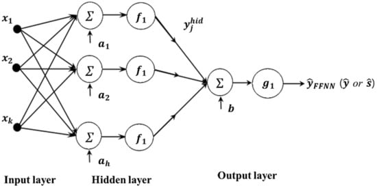
Figure 2.
Proposed FFNN-based RD modeling method.
The input layer has control factors, , …, , …, . The input for each hidden neuron is the weighted sum of these factors plus their associated bias, expressed as . This calculated value will be transformed by a transformation function (), also called an activation function (expressed by Equation (5)). The transformed value is both the output of the hidden neuron and the input for the next layer (in our case, the output layer). Subsequently, the ultimate transformed outcome is the final result. The outputs of the hidden neuron and FFNN can then be expressed as
where is the weight connecting input factor to hidden node j; is the associated bias of the hidden layer node j, and is the transfer function of the hidden layer.
where is the activation function of the output layer, h is the number of hidden nodes, is the weight connecting each hidden node to the output layer, and is the output bias.
The typical transfer functions for the hidden and output layers are the hyperbolic tangent sigmoid and linear functions, respectively. The estimated mean and standard deviation functions in this case are
where and represent the number of hidden neurons in the mean and standard deviation estimation model, respectively. Moreover, and represent the bias for hidden node in both models, while and denote the bias of the output neuron. Similarly, and signify the weight connecting a hidden node to the output for both models, while and refer to the weight connecting the input factors to a hidden node of the FFNN estimation model for mean and standard deviation, respectively.
2.2.2. Number of Hidden Neurons
For a NN model with a single hidden layer, the number of neurons in the hidden layer must be chosen carefully since use of a larger number of hidden neurons can generate a model that more accurately reflects the training data. However, use of a large number of hidden neurons makes the model increasingly complex and may lead to overfitting. On the flip side, use of only a few hidden neurons may cause underfitting. Several researchers have proposed approaches to determine the ideal number of hidden neurons. A review that discusses how to fix the number of hidden neurons in NNs was presented by Sheela and Deepa [54], but no single method is effective in every circumstance. In this paper, the well-established Schwartz’s Bayesian criterion, or the Bayesian information criterion (BIC), is used to determine the number of hidden neurons. This criterion is defined as
where n and denote the sample size and the number of parameters, respectively. In BIC, the term generally penalizes free parameters strongly. In addition, the accuracy of the NN model will increase as the sample size increases.
2.2.3. Integration into a Learning Algorithm: Back-Propagation
NN-based estimation requires a learning algorithm, such as error correction, perception learning, Boltzmann learning, Hebbian rules, or back-propagation (BP). Among these, BP is one of the most popular network training algorithms because it is both simple and generally applicable [55]. The back-propagation algorithm trains a NN by applying the chain rule method. The weights of the network are randomly initialized, then repeatedly adjusted through minimization of the cost function, which is calculated by measuring the difference between the actual output and the desired value . One of the most common error measures is the root mean square (RMS) error, defined by
During the training process, the RMS error (cost function) is minimized as much as possible. The iterative step of the gradient descent algorithm then changes the weights according to
Here, is the learning rate, which can determine the effect of the gradient. There are a few alternative optimization techniques for finding the local minimum, such as conjugate gradient, steepest descent, and Newton’s method.
- Steepest descent is an iterative method that finds the local minimum by moving in the direction opposite to the one implied by the gradient; the learning rate (such as traingda or traingdx) indicates how quickly it moves. Usually, the smaller the learning rate, the slower the process of convergence to a local minimum. In standard steepest descent, the learning rate remains constant throughout the training stage while the weight and bias parameter values are interactively updated.
- The resilientBP training algorithm (i.e., trainrp) is a local adaptive learning scheme for supervised batch learning in an FFNN. Resilient back-propagation is similar to the standard BP algorithm, but it is capable of training the NN model faster than the regular method without the need to specify any free parameter values. Additionally, since trainrp merely considers the size of the partial derivatives, the direction of the weight update is only affected by the sign of the derivative.
- The Levenberg-Marquardt algorithm (i.e., trainlm) is a standard method for solving nonlinear least-squares minimization problems without computing the Hessian matrix. It can be thought of as a middle ground between the steepest descent and Gauss-Newton methods.
2.2.4. Generalization and Overfitting Issues
NN models are often used in order to generalize the information learned from the training data to any unseen data so that it is possible to make inferences or predictions for the problem domain. Nevertheless, overfitting can occur, in which case a trained NN model will work correctly on the training data but perform terribly on test data. Overfitting can happen when the model is too complicated or has too many parameters. To avoid this problem, the additional technique of “early stopping” is often used to improve the generalizability of the model. With an early stopping mechanism, the training process can be halted in an early iteration to prevent overfitting. Normally, to ensure the accuracy and efficiency of the NN model, the whole dataset should be divided into three subsets: the training, validation, and test datasets. Training data is used for NN model construction, while validation and test data are applied to check the model’s error and efficiency, respectively. The exact proportions of the training, test, and validation datasets are determined by the designer; the most widely used ratios are 50:25:25 or 60:20:20. In this technique, the optimal point at which to stop training is indicated by the minimum estimated true error, as shown in Figure 3 [56].
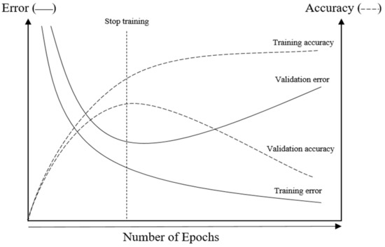
Figure 3.
Early stopping technique.
2.3. Proposed NN-Based Estimation Method 2: CFNN Structure
An alternative NN-based model, the cascade forward neural network (CFNN), has been shown to boost model accuracy and learning speed in cases with complicated relationships. CFNN is similar to FFNN, except that the former also includes a weighted link between the input and output layers. The additional connection means that the inputs can directly affect the output, which increases the complexity of the model but also increases its accuracy. Likewise, the CFNN model uses the BP algorithm to update the weights but has a drawback in that each layer of neurons is related to all previous layers of neurons [57]. The proposed CFNN-based modeling method is illustrated in Figure 4. The output of CFNN is expressed as follows:
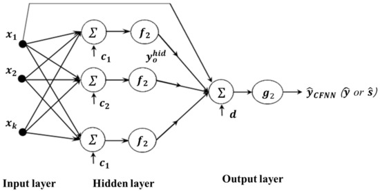
Figure 4.
Proposed CFNN-based RD modeling method.
Again, the hyperbolic tangent sigmoid and linear functions are usually used as the transfer functions in the hidden and output layers, respectively. In this case, the derived mean and standard deviation functions are expressed as
where and , and , and , and , and , , and denote the number of hidden neurons, bias at hidden node , bias at the output neuron, weight connecting hidden node to the output neuron, weight connecting input factor to hidden node , and weights directly linking input factor to the output neuron of the CFNN for the mean and standard deviation, respectively.
2.4. Proposed NN-Based Estimation Method 3: RBFN
RBFN generally gives excellent, fast approximations for curve-fitting problems. This multilayer feed-forward NN has a single hidden layer and uses radial basis activation functions in the hidden neurons. The radial basis function (kernel) is a function whose value depends on the distance between the input value and center points, where the centers and width can be determined by methods such as random selection, k-means clustering, supervised selection, unsupervised learning, etc. [58]. Unlike in an FFNN, the output of the hidden neuron is given by the product of the bias and the Euclidean distance between the input and weight vectors. Figure 5 shows the RBFN structure used to estimate the process mean and standard deviation functions.
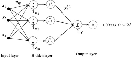
Figure 5.
Proposed RBFN-based RD modeling method. The operation “*” denotes the element-by-element multiplication.
In this essay, the design of an RBFN requires a two-step training procedure. First, the kernel positions, kernels widths, and weights that link the hidden layer inputs to the output layer nodes are estimated using an unsupervised LMS algorithm. After this initial solution has been obtained, a supervised gradient-based algorithm can then be used to refine the network parameters. The dispersion constant, or spread, exhibits a strong relationship with the output of the network. Specifically, the input region covers a large area when the spread is vast; if the spread is relatively narrow, the radial basis function curve is steeper, and the neuron output is much more significant relative to the weighted input vector approach. As a result, the network output is closer to the expected output [59]. The output of RBFN is expressed as
In this case, the estimated mean and standard deviation functions are
where , , , , , , , , , and denote the number of hidden neurons, bias at hidden node , bias at the output neuron, weight connecting hidden node to the output, and weight connecting input factor to hidden node of RBFN for the mean and standard deviation, respectively.
3. Simulation Studies
A variety of simulation-based examples are presented to demonstrate the efficacy of the NN-based RD modeling methods. Assume that a given exact function representing the true relationship between the input factors and output response is represented as
The factorial design is used to evaluate how two factors with five levels impact one response. The related experimental data are exhibited in Table 1, and the actual relationship function is shown in Equation (18). Figure 6 shows a plot of the experimental data and true response value. The replicated response value is created at each treatment level by randomly adding some deviation from the true response value. In this paper, two different simulation studies are conducted to check the efficiency of our proposed model.

Table 1.
Experimental data and true function response value.
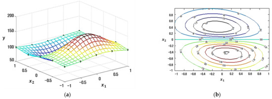
Figure 6.
Sampled points on the true response surface. (a) Surface plot. (b) Contour plot.
In RD, the expected quality loss (EQL) is often used as a critical optimization criterion to compare different methods. The EQL is given by
where denotes the loss coefficient, normally , and , , and represent the estimated mean function, approximated standard deviation function, and target value, respectively. In both simulation studies, the target value is defined as 128 ().
3.1. Simulation Study 1
Simulation study 1 was conducted by randomly adding a number of small standard deviation values to the true response to give 50 replicates of the output response. Experimental data from simulation study 1 are presented in Table 2.

Table 2.
Experimental data from simulation study 1.
The approximated mean and standard deviation functions shown in Equations (20) and (21) were estimated using the LSM-based RSM method in MATLAB software.
Information about the trained multilayer feed-forward NN model, including the transfer function and NN architecture (number of inputs, number of hidden neurons, number of outputs), is given in Table 3 and Table 4. Furthermore, the weight and bias values associated with each layer of the three proposed NN models (FFNN, CFNN, and RBFN) for both the process mean and standard deviation function estimations are exhibited in Appendix A (Table A1, Table A2, Table A3 and Table A4, respectively).

Table 3.
Summary of multilayer feed-forward NN information for simulation 1.

Table 4.
Summary of RBFN information for simulation 1.
The conventional LSM-based RSM method is compared to the proposed FFNN-, CFNN-, and RBFN-based RD modeling methods in Figure 7, Figure 8, Figure 9 and Figure 10 in contour plot form. Furthermore, Table 5 shows the ultimate solution set and corresponding best response values, while the comparison is done in terms of EQL.
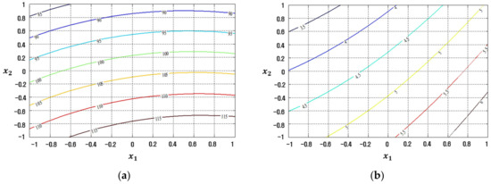
Figure 7.
Response plots created using the conventional LSM-based RSM in simulation study 1: (a) Mean (R2 = 29.54%), (b) Standard deviation (R2 = 86.61%).
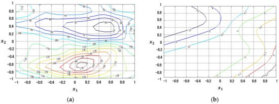
Figure 8.
Response plots created using the proposed FFNN-based modeling method in simulation study 1: (a) Mean (R2 = 89.96%), (b) Standard deviation (R2 = 89.28%).
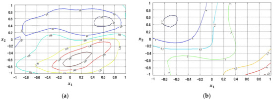
Figure 9.
Response plots created using the proposed CFNN-based modeling method in simulation study 1: (a) Mean (R2 = 83.22%), (b) Standard deviation (R2 = 86.68%).
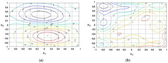
Figure 10.
Response plots created using the proposed RBFN-based modeling method in simulation study 1: (a) Mean (R2 = 99.99%), (b) Standard deviation (R2 = 99.99%).

Table 5.
Comparative results in simulation study 1.
The results in Table 5 clearly show that the proposed RD modeling approach with the three NN architectures produces much smaller EQL values than the approach using LSM-based RSM. Specifically, both the process bias and variance values obtained from the proposed NN-based model are significantly lower than those of LSM-based RSM. The squared process bias vs. variance results of the conventional LSM-based RSM and proposed FFNN-, CFNN-, and RBFN-based modeling methods in simulation study 1 are illustrated in Figure 11. The optimal settings are marked with green stars in each figure.
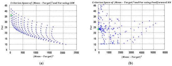
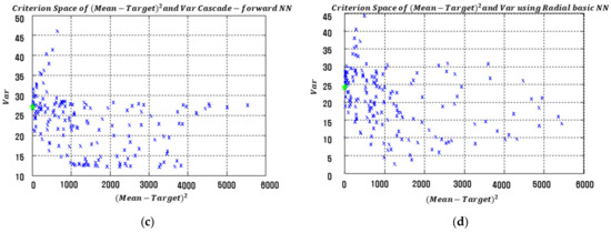
Figure 11.
Criterion space of the estimated functions in simulation study 1. (a) LSM-based RSM. (b) Proposed FFNN. (c) Proposed CFNN. (d) Proposed RBFN.
3.2. Simulation Study 2
Simulation study 2 was conducted by randomly adding a number of large standard deviation values to the true response to give 50 replicates. The experimental data of simulation study 2 are presented in Table 6. The estimated mean and standard deviation functions given by LSM-based RSM in simulation study 2 are:

Table 6.
Experimental data for simulation 2.
Similarly, detailed information about the multilayer FFNN is given in Table 7 and Table 8, while the weight and bias values of all proposed models for both the process mean and standard deviation functions are summarized in Appendix B (Table A5, Table A6, Table A7 and Table A8). Contour plots of the process mean and standard deviation response values for each model are displayed in Figure 12, Figure 13, Figure 14 and Figure 15, respectively.

Table 7.
Summary of the multilayer FFNN in simulation 2.

Table 8.
Summary of the RBFN in simulation 2.
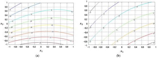
Figure 12.
Response plots created using the conventional LSM-based RSM in simulation study 2: (a) Mean (R2 = 32.04%), (b) Standard deviation (R2 = 91.36%).
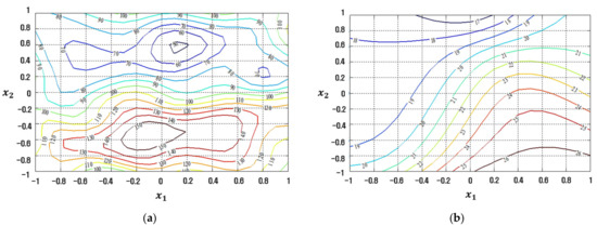
Figure 13.
Response plots created using the proposed FFNN-based modeling method in simulation study 2: (a) Mean (R2 = 90.76%), (b) Standard deviation (R2 = 91.36%).
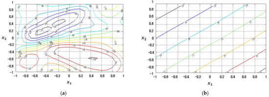
Figure 14.
Response plots created using the proposed CFNN-based modeling method in simulation study 2: (a) Mean (R2 = 80.98%), (b) Standard deviation (R2 = 89.32%).
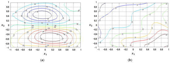
Figure 15.
Response plots created using the proposed RBFN-based modeling method in simulation study 2: (a) Mean (R2 = 99.99%), (b) Standard deviation (R2 = 99.99%).
Table 9 presents the optimal input factor settings, associated process mean, process bias, process variance, and EQL values obtained from the proposed NN-based modeling methods and LSM-based RSM in simulation study 2. The proposed NN-based modeling methods again produced significantly smaller EQL values than the LSM-based RSM. The plot of squared process bias vs. the variance for LSM-based RSM and the proposed FFNN-, CFNN-, and RBNN-based modeling methods are illustrated in Figure 16. The optimal settings are marked with green stars in each figure.

Table 9.
Comparative results of simulation study 2.
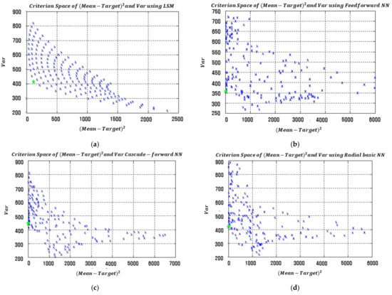
Figure 16.
Criterion space of the estimated functions in simulation study 2. (a) LSM-based RSM. (b) Proposed FFNN. (c) Proposed CFNN. (d) Proposed RBFN.
Clearly, the proposed NN-based modeling methods produced better solutions than LSM-based RSM in both simulation studies. Whereas RSM is generally used to estimate second-order functions, the proposed modeling methods can effectively estimate nonlinear functions.
4. Case Study
The printing data example used by Vining and Myers [6] and Lin and Tu [9] was selected to demonstrate the application of the proposed methods. The printing experiment investigates the effects of speed (), pressure (), and distance () on a printing machine’s ability to add colored ink to a package (y). The case study has a factorial design with three level three factors, so in total, the number of experimental runs is . To ensure the accuracy of the experiment, each treatment combination is repeated three times. In this case study, the target . The experimental data are given in Vining and Myers [6]. The estimated mean and standard deviation functions given by LSM-based RSM are
where , , , , and .
The information used for the RD modeling methods after training with the associated transfer functions, training functions, NN architectures (number of inputs, number of hidden neurons, number of outputs), and number of epochs in the case study are summarized in Table 10 and Table 11. The specified weight and bias values of the proposed FFNN, DFNN, and RBFN used to approximate the process mean and standard deviation functions in the case study are shown in Appendix C (Table A9, Table A10, Table A11, Table A12, Table A13 and Table A14).

Table 10.
Summary of the multilayer FFNN used in the case study.

Table 11.
Summary of the RBFN used in the case study.
The contour plots of the response functions for the process mean and standard deviation estimated by the LSM-based RSM, FFNN, CFNN, and RBFN robust design modeling methods are demonstrated in Figure 17, Figure 18, Figure 19 and Figure 20, respectively.
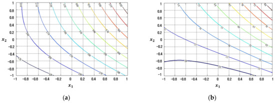
Figure 17.
Response plots created using the conventional LSM-based RSM in the case study: (a) Mean (R2 = 92.68%), (b) Standard deviation (R2 = 45.42%).
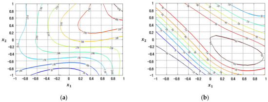
Figure 18.
Response plots created using the proposed FFNN-based modeling method in the case study: (a) Mean (R2 = 91.70%), (b) Standard deviation (R2 = 73.51%).
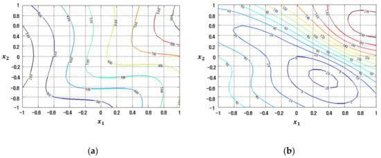
Figure 19.
Response plots created using the proposed CFNN-based modeling method in the case study: (a) Mean (R2 = 83.05%), (b) Standard deviation (R2 = 69.47%).
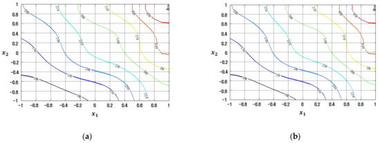
Figure 20.
Response plots created using the proposed RBFN-based modeling method in the case study: (a) Mean (R2 = 99.99%), (b) Standard deviation (R2 = 99.99%).
Table 12 presents the optimal factor settings, associated process mean, process bias, process variance, and EQL values obtained from the proposed NN-based modeling methods and LSM-based RSM in the case study. The proposed RD modeling methods produced significantly smaller EQL values than LSM-based RSM.

Table 12.
Comparative results of the case study.
The process variance obtained from the proposed NN-based estimation methods is markedly lower than that of conventional RSM. The scatter plots demonstrate the value of squared process bias vs. variance for the traditional LSM-based RSM model and the three proposed NN-based modeling methods as illustrated in Figure 21. The optimal settings are marked with green stars in each figure.
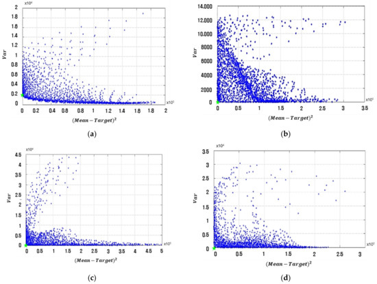
Figure 21.
Criterion space of the estimated functions in the case study. (a) LSM-based RSM. (b) Proposed FFNN. (c) Proposed CFNN. (d) Proposed RBFN.
5. Conclusions and Further Studies
This paper identified three NN-based modeling approaches (FFNN, CFNN, and RBFN) that obviate the need for the assumptions required when LSM-based RSM is used to approximate the mean and standard deviation functions. The feed-forward NN structure-based RD modeling methods are alternative options for identifying a functional relationship between input factors and process mean and standard deviation in RD. Compared with the conventional RD modeling method, the proposed approach has significant advantages with regard to accuracy and efficiency. The proposed RD modeling methods can easily be implemented using existing software such as MATLAB. The results of both the two types of simulation studies and case study show that the proposed RD modeling methods provide better optimal solutions than conventional LSM-based RSM. The main results are summarized, and the variability index, EQL, and R2 are central to the model validation criteria. (i) In simulation study 1, the proposed RD modeling methods showed, on average, 139 times lower process bias and 1.5 times lower process variance than LSM-based RSM in terms of variability, and about four times smaller in EQL. Moreover, among the three NN-Based modelings, FFNN showed the lowest value in terms of EQL. (ii) In simulation study 2, the proposed RD modeling methods showed 11 times lower process bias and one time lower process variance than LSM-based RSM on average in terms of variability and about 1.2 times smaller in EQL. Among the three NN-Based modelings, FFNN also showed the lowest value. (iii) In the case study, the proposed RD modeling methods showed significantly lower results than LSM-based RSM, with an average process bias of 102 times and process variance of 85 times in terms of variability, and about 86 times smaller in EQL. Among the three NN-Based modelings, CFNN and FFNN showed much lower values than RBFN. (iv) Specifically, in the printing machine case study, the R2 values for the estimated standard deviation functions are 45.452%, 73.51%, 69.47%, and 99.99%, when the conventional LSM-based RSM, FFNN-based modeling, CFNN-based modeling and RBFN-based modeling methods are applied respectively.
In future work, the proposed NN structures-based RD methods could be used to estimate multiple responses (RD multi-objective optimization problem), time-series data, big data, and simulation data [60]. But the activation and transfer function in the hidden and output layers should be carefully investigated and selected separately when applied. In addition, in this study, a classical case study was performed to verify the proposed methodology, but in the future study, a field-based case study that suggests optimal process conditions for productivity improvement in a smart factory will be performed.
Author Contributions
Conceptualization, T.-H.L. and S.S.; Methodology, T.-H.L. and S.S.; Modeling, T.-H.L.; Validation T.-H.L. and S.S.; Writing—Original Draft Preparation, T.-H.L. and S.S.; Writing—Review and Editing, L.D., H.J. and S.S.; Funding Acquisition, H.J. All authors have read and agreed to the published version of the manuscript.
Funding
This work was supported by the National Research Foundation of Korea (NRF) (No. NRF-2019R1G1A1010335).
Conflicts of Interest
The authors declare no conflict of interest.
Appendix A. Weight and Bias Values of the Proposed Neural Network Structure in Simulation Study 1

Table A1.
Estimated parameter values (Weight and bias) of the proposed FFNN for simulation study 1.
Table A1.
Estimated parameter values (Weight and bias) of the proposed FFNN for simulation study 1.
| a. Mean Function | ||||
| Weights | Biases | |||
| 3.6550 | 4.7000 | −0.5320 | −5.6150 | −0.3370 |
| 4.6370 | 3.2890 | 0.7650 | −5.1200 | |
| −3.6880 | 4.6390 | 0.3910 | 4.1080 | |
| 5.4630 | 1.9730 | −0.1880 | −3.5370 | |
| 1.3880 | −5.7220 | 0.2690 | −2.5120 | |
| −4.3340 | 3.7490 | −0.2760 | 2.2050 | |
| −2.5860 | 5.1880 | −0.1570 | 1.3530 | |
| 1.4470 | 5.5880 | −0.3560 | −0.7180 | |
| 4.9970 | 2.8280 | 0.1800 | −0.0290 | |
| 5.1210 | 2.5860 | −0.1410 | 0.8320 | |
| −5.5550 | −1.5900 | −0.4130 | −1.4570 | |
| 5.4750 | 1.8190 | −0.2640 | 2.1750 | |
| 4.6360 | −3.3980 | 0.0280 | 2.9310 | |
| −0.4150 | 5.7380 | 0.4640 | −3.6420 | |
| 3.1110 | −4.8490 | 0.0690 | 4.3330 | |
| −4.8490 | −2.9730 | −0.0830 | −5.0940 | |
| −1.0380 | −5.9250 | −0.5680 | −5.5340 | |
| b. Standard Deviation Function | ||||
| Weights | Biases | |||
| 2.3640 | −2.2900 | 0.6380 | −3.2240 | 0.5100 |
| 3.1150 | 3.1890 | 0.2420 | −1.9530 | |
| −1.9210 | 1.7710 | 0.1340 | 2.8660 | |
| 0.7590 | 5.2410 | −0.0100 | 1.6240 | |
| 1.4680 | −3.0400 | 0.4510 | 1.2370 | |
| 0.8010 | 2.7570 | 0.1990 | −3.3430 | |

Table A2.
Estimated parameter values (Weight and bias) of the proposed CFNN for mean function in simulation study 1.
Table A2.
Estimated parameter values (Weight and bias) of the proposed CFNN for mean function in simulation study 1.
| Weights | Biases | ||||
|---|---|---|---|---|---|
| 3.4680 | 4.5940 | 0.5890 | −5.7880 | −0.3310 | |
| 4.7000 | 3.4200 | −0.1830 | −5.0120 | ||
| −3.5790 | 4.9050 | 0.5820 | 3.9430 | ||
| 5.2270 | 2.2140 | −0.1130 | −3.7440 | ||
| 1.5730 | −5.5360 | 0.2110 | −2.9200 | ||
| −4.3610 | 3.8520 | −0.5380 | 2.0050 | ||
| −2.6110 | 5.1060 | −0.2640 | 1.4290 | ||
| 1.3240 | 5.6320 | −0.2540 | −0.3850 | −0.8230 | |
| 5.0350 | 2.7780 | 0.3700 | −0.2030 | 0.3890 | |
| 5.1120 | 2.6770 | 0.0370 | 0.7280 | ||
| −5.4880 | −1.8040 | −0.0510 | −1.4370 | ||
| 5.4600 | 1.8770 | 0.1170 | 2.1230 | ||
| 4.5330 | −3.4080 | 0.3510 | 3.1740 | ||
| −0.6110 | 5.8300 | 0.0350 | −3.4760 | ||
| 3.1690 | −4.8040 | −0.3720 | 4.4170 | ||
| −4.9220 | −3.0140 | −0.0030 | −5.0410 | ||
| −0.9670 | −5.6650 | −0.5560 | −5.7940 | ||

Table A3.
Estimated parameter values (Weight and bias) of the proposed CFNN for standard deviation function in simulation study 1.
Table A3.
Estimated parameter values (Weight and bias) of the proposed CFNN for standard deviation function in simulation study 1.
| Weights | Biases | ||||
|---|---|---|---|---|---|
| 1.9650 | −1.2350 | −0.1600 0.1370 | 0.9570 | −3.1820 | 0.9310 |
| 2.8420 | −1.4330 | 0.3030 | 1.1660 | ||
| −2.7860 | −0.2660 | −0.3060 | 0.4420 | ||
| 1.7340 | 3.2990 | −0.4380 | 1.9590 | ||
| 0.6130 | 3.8920 | 0.1590 | 3.1660 | ||

Table A4.
Estimated parameter values (Weight and bias) of the proposed RBFN in simulation study 1.
Table A4.
Estimated parameter values (Weight and bias) of the proposed RBFN in simulation study 1.
| a. Mean Function | b. Standard Deviation Function | ||||||||
|---|---|---|---|---|---|---|---|---|---|
| Weights | Biases | Weights | Biases | ||||||
| 0.0 | −0.5 | 126.7450 | 1.3870 | 31.5280 | 0.5 | −0.5 | 6.8760 | 1.3870 | 33.6620 |
| 0.5 | 1.0 | −29.6660 | 1.3870 | 0.5 | 1.0 | −3.6160 | 1.3870 | ||
| −1.0 | 0.5 | 9.1310 | 1.3870 | −1.0 | −0.5 | 3.9420 | 1.3870 | ||
| 1.0 | −0.5 | −35.0720 | 1.3870 | −1.0 | 1.0 | −28.7180 | 1.3870 | ||
| −1.0 | −1.0 | 55.8470 | 1.3870 | 1.0 | −1.0 | −24.2000 | 1.3870 | ||
| 1.0 | 1.0 | 72.6050 | 1.3870 | 1.0 | 0.5 | 0.1440 | 1.3870 | ||
| −0.5 | 1.0 | 7.0470 | 1.3870 | −0.5 | −0.5 | 8.5470 | 1.3870 | ||
| −0.5 | 0.5 | −52.0380 | 1.3870 | 0.0 | 0.5 | −11.9050 | 1.3870 | ||
| −1.0 | 0.0 | 31.4830 | 1.3870 | −0.5 | −1.0 | 0.5760 | 1.3870 | ||
| 1.0 | −1.0 | 77.7170 | 1.3870 | −1.0 | 0.5 | 5.4580 | 1.3870 | ||
| 1.0 | 0.0 | 79.6550 | 1.3870 | 0.5 | 0.5 | 11.8210 | 1.3870 | ||
| −1.0 | 1.0 | 56.6220 | 1.3870 | 0.0 | 0.0 | −4.1700 | 1.3870 | ||
| 0.5 | 0.5 | 43.0670 | 1.3870 | 0.0 | 1.0 | −16.5340 | 1.3870 | ||
| 0.0 | 1.0 | 92.4890 | 1.3870 | 1.0 | 1.0 | −23.5990 | 1.3870 | ||
| −1.0 | −0.5 | 13.2020 | 1.3870 | 1.0 | 0.0 | −21.1190 | 1.3870 | ||
| −0.5 | −0.5 | −60.8050 | 1.3870 | 0.0 | −1.0 | −18.9870 | 1.3870 | ||
| 0.0 | 0.5 | −59.6330 | 1.3870 | 0.5 | 0.0 | −9.2400 | 1.3870 | ||
| −0.5 | 0.0 | 65.2090 | 1.3870 | −1.0 | 0.0 | −25.1250 | 1.3870 | ||
| −0.5 | −1.0 | 11.5900 | 1.3870 | 0.0 | −0.5 | −9.8510 | 1.3870 | ||
| 0.0 | 0.0 | −2.2410 | 1.3870 | −0.5 | 0.0 | −7.7680 | 1.3870 | ||
| 0.5 | −1.0 | −31.3730 | 1.3870 | 1.0 | −0.5 | 2.7330 | 1.3870 | ||
| 1.0 | 0.5 | −27.4060 | 1.3870 | −1.0 | −1.0 | −27.3400 | 1.3870 | ||
| 0.5 | −0.5 | 51.3100 | 1.3870 | 0.5 | −1.0 | 0.6880 | 1.3870 | ||
| 0.5 | 0.0 | −51.9210 | 1.3870 | −0.5 | 0.5 | 6.3400 | 1.3870 | ||
Appendix B. Weight and Bias Values of the Proposed Neural Network Structure in Simulation Study 2

Table A5.
Estimated parameter values (Weight and bias) of the proposed FFNN in simulation study 2.
Table A5.
Estimated parameter values (Weight and bias) of the proposed FFNN in simulation study 2.
| a. Mean Function | b. Standard Deviation Function | ||||||||
|---|---|---|---|---|---|---|---|---|---|
| Weights | Biases | Weights | Biases | ||||||
| 2.0570 | 3.9280 | 0.7630 | −4.7780 | 0.0530 | 1.7820 | 1.8550 | −0.3890 | −1.6150 | 0.6640 |
| 2.4000 | 3.9130 | 0.4830 | −3.4680 | 2.2310 | −0.7030 | 0.5740 | 0.0480 | ||
| −4.5010 | −0.4190 | 0.5650 | 3.0550 | −0.2220 | −1.8100 | 1.0090 | −2.9250 | ||
| 2.9150 | 3.7590 | 0.2290 | −1.3400 | ||||||
| 1.4850 | −4.3180 | 0.9410 | −1.3350 | ||||||
| −4.6270 | −0.2660 | 0.6220 | −0.1490 | ||||||
| −2.2500 | 3.9870 | −0.6890 | −1.0590 | ||||||
| 0.7070 | 4.5580 | 0.1550 | 1.5870 | ||||||
| 2.6160 | 3.8280 | 0.5310 | 2.4090 | ||||||
| 4.3540 | 1.5560 | −0.9940 | 4.0990 | ||||||
| −2.6170 | −3.7890 | −1.3930 | −4.6190 | ||||||

Table A6.
Estimated parameter values (Weight and bias) of the proposed CFNN for mean function in simulation study 2.
Table A6.
Estimated parameter values (Weight and bias) of the proposed CFNN for mean function in simulation study 2.
| Weights | Biases | ||||
|---|---|---|---|---|---|
| 5.1170 | −0.1120 | 0.3710 0.8340 | −0.3840 | −4.9710 | 0.0220 |
| 4.2260 | 2.9460 | 0.2340 | −4.0130 | ||
| −3.7930 | −3.5990 | 0.0640 | 3.0950 | ||
| 4.5130 | −0.8420 | −0.0300 | −3.2350 | ||
| 1.8880 | 4.7280 | −0.2380 | −1.5650 | ||
| −4.2200 | 2.7300 | 0.0610 | 0.9880 | ||
| −1.7950 | 4.8310 | −0.4210 | 0.2780 | ||
| 1.5620 | 4.7170 | −0.5560 | 0.9210 | ||
| 3.5040 | −3.6720 | 0.5150 | 1.6860 | ||
| 4.1320 | 2.8270 | 0.2500 | 2.6160 | ||
| −3.2120 | 4.0320 | 0.5630 | −3.1850 | ||
| 4.8210 | 1.5590 | −0.5310 | 4.0190 | ||
| 4.4480 | 2.5990 | 0.2130 | 4.9300 | ||

Table A7.
Estimated parameter values (Weight and bias) of the proposed CFNN for standard deviation function in simulation study 2.
Table A7.
Estimated parameter values (Weight and bias) of the proposed CFNN for standard deviation function in simulation study 2.
| Weights | Biases | ||||
|---|---|---|---|---|---|
| 1.2450 | 0.7210 | 0.5230 −0.5240 | −0.0310 | 0.2590 | −0.0380 |

Table A8.
Estimated parameter values (Weight and bias) of the proposed RBFN in simulation study 2.
Table A8.
Estimated parameter values (Weight and bias) of the proposed RBFN in simulation study 2.
| a. Mean Function | b. Standard Deviation Function | ||||||||
|---|---|---|---|---|---|---|---|---|---|
| Weights | Biases | Weights | Biases | ||||||
| 0.0 | −0.5 | 64.8980 | 1.6650 | 38.201 | 0.5 | −0.5 | −28.2270 | 1.3870 | −1.6450 |
| 0.5 | 1.0 | −6.6220 | 1.6650 | −0.5 | 0.5 | 8.2530 | 1.3870 | ||
| −1.0 | 0.5 | 17.0920 | 1.6650 | 1.0 | 1.0 | 21.6710 | 1.3870 | ||
| 1.0 | −0.5 | −8.6860 | 1.6650 | −1.0 | −1.0 | 34.5170 | 1.3870 | ||
| −1.0 | −1.0 | 34.9310 | 1.6650 | 1.0 | −1.0 | 9.1260 | 1.3870 | ||
| 1.0 | 0.5 | −21.9170 | 1.6650 | −0.5 | −1.0 | −17.9100 | 1.3870 | ||
| −0.5 | 1.0 | 25.6960 | 1.6650 | 1.0 | 0.0 | −5.4440 | 1.3870 | ||
| 0.5 | −1.0 | 10.9180 | 1.6650 | 0.0 | −1.0 | 22.5250 | 1.3870 | ||
| −1.0 | 0.0 | 26.8410 | 1.6650 | 0.5 | 1.0 | −3.2470 | 1.3870 | ||
| −1.0 | 1.0 | 31.4250 | 1.6650 | −1.0 | 0.0 | 32.0960 | 1.3870 | ||
| −0.5 | −1.0 | 34.7400 | 1.6650 | −1.0 | 1.0 | 17.5940 | 1.3870 | ||
| 1.0 | 1.0 | 62.8200 | 1.6650 | 0.0 | 0.5 | 4.8550 | 1.3870 | ||
| 0.5 | 0.0 | −47.0190 | 1.6650 | −0.5 | 0.0 | −11.1920 | 1.3870 | ||
| 1.0 | −1.0 | 40.4510 | 1.6650 | 0.0 | 1.0 | 12.6800 | 1.3870 | ||
| 1.0 | 0.0 | 63.1560 | 1.6650 | −1.0 | −0.5 | −25.7220 | 1.3870 | ||
| 0.0 | 1.0 | 55.4460 | 1.6650 | 1.0 | 0.5 | 4.0170 | 1.3870 | ||
| −0.5 | −0.5 | −4.6920 | 1.6650 | 0.5 | 0.5 | −7.4010 | 1.3870 | ||
| 0.5 | −0.5 | 62.5500 | 1.6650 | −0.5 | −0.5 | 20.5440 | 1.3870 | ||
| −0.5 | 0.0 | 17.0590 | 1.6650 | 1.0 | −0.5 | 26.7630 | 1.3870 | ||
| −0.5 | 0.5 | −11.3100 | 1.6650 | 0.5 | 0.0 | 27.5990 | 1.3870 | ||
| −1.0 | −0.5 | 21.5900 | 1.6650 | 0.5 | −1.0 | 13.4280 | 1.3870 | ||
| 0.5 | 0.5 | 52.6940 | 1.6650 | −1.0 | 0.5 | −12.6070 | 1.3870 | ||
| 0.0 | 0.5 | −59.7970 | 1.6650 | −0.5 | 1.0 | −3.6890 | 1.3870 | ||
| 0.0 | 0.0 | 35.7290 | 1.6650 | 0.0 | −0.5 | 3.9230 | 1.3870 | ||
Appendix C. Weight and Bias Values of the Proposed Neural Network Structure in the Case Study

Table A9.
Estimated parameter values (Weight and bias) of the FFNN for mean function in the case study.
Table A9.
Estimated parameter values (Weight and bias) of the FFNN for mean function in the case study.
| Weights | Biases | ||||
|---|---|---|---|---|---|
| 1.5660 | 1.9450 | 1.1790 | 0.3610 | −3.0880 | −0.1520 |
| 1.7450 | −1.3140 | 2.0400 | 0.4270 | −2.0620 | |
| −1.6810 | 2.2590 | 0.6690 | 0.2180 | 1.4730 | |
| 1.5770 | 1.7570 | −1.5510 | 0.1660 | −0.9160 | |
| 1.1460 | −0.0730 | 2.6140 | 0.0510 | 0.1540 | |
| −1.7480 | 1.4660 | 1.7830 | −0.0630 | −0.4130 | |
| −1.3760 | −2.3660 | 0.9550 | −0.1300 | −1.4310 | |
| 0.5280 | −0.8930 | 2.4800 | 0.2700 | 2.4590 | |
| 1.9980 | 1.7550 | 1.2700 | −0.0220 | 2.8680 | |

Table A10.
Estimated parameter values (Weight and bias) of the FFNN for standard deviation function in the case study.
Table A10.
Estimated parameter values (Weight and bias) of the FFNN for standard deviation function in the case study.
| Weights | Biases | ||||
|---|---|---|---|---|---|
| 1.9520 | −2.0810 | 0.9550 | −0.2470 | −3.0060 | −0.3080 |
| 1.4520 | 1.6590 | −1.9370 | −0.5730 | −2.5620 | |
| −1.6750 | 1.9270 | 1.5750 | −0.0660 | 1.6940 | |
| 1.9030 | −0.2630 | 2.2310 | 0.1620 | −1.0300 | |
| 0.9430 | 2.3320 | 1.6200 | 0.1020 | −0.3810 | |
| −2.0160 | −1.7170 | 1.3500 | −0.2570 | −0.1860 | |
| −1.9130 | −0.4820 | 2.2770 | 0.0650 | −0.9540 | |
| 0.2000 | 2.8330 | −0.8230 | 0.1420 | 1.7220 | |
| 2.7580 | 1.5070 | 0.6520 | 0.3000 | 1.9940 | |
| 1.497 | 1.726 | −1.141 | −0.938 | 3.480 | |

Table A11.
Estimated parameter values (Weight and bias) of the CFNN for mean function in the case study.
Table A11.
Estimated parameter values (Weight and bias) of the CFNN for mean function in the case study.
| Weights | Biases | |||||
|---|---|---|---|---|---|---|
| 1.7480 | 2.4100 | 1.0820 | 0.5820 0.1600 0.6080 | −0.0060 | −3.2030 | 0.1530 |
| 2.6590 | −0.1570 | 1.7430 | −0.1080 | −2.6440 | ||
| −2.1980 | 1.7500 | 1.4620 | −0.2100 | 2.0920 | ||
| 2.3100 | −1.9110 | −0.7440 | 0.0770 | −1.6370 | ||
| 1.9620 | −0.9270 | 2.3510 | −0.0110 | −0.8430 | ||
| −1.9680 | 1.8610 | −1.6700 | −0.0560 | 0.2480 | ||
| −1.5170 | 2.3360 | 1.6270 | 0.4240 | −0.2960 | ||
| 0.2480 | 2.1750 | −2.3370 | 0.0730 | 0.8240 | ||
| 2.7660 | 0.9810 | −1.3500 | −0.0010 | 1.3920 | ||
| 1.8210 | −1.8120 | −1.8440 | 0.2630 | 2.0910 | ||
| −1.6870 | 1.7400 | −2.0190 | 0.2820 | −2.6670 | ||
| 2.1030 | 1.8880 | 1.2460 | −0.5660 | 3.3270 | ||

Table A12.
Estimated parameter values (Weight and bias) of the CFNN for standard deviation function in the case study.
Table A12.
Estimated parameter values (Weight and bias) of the CFNN for standard deviation function in the case study.
| Weights | Biases | |||||
|---|---|---|---|---|---|---|
| 2.0800 | 2.0450 | 1.7150 | −0.4480 −0.6100 0.7170 | 0.8060 | −2.7520 | −0.0920 |
| 1.3360 | 2.1850 | 1.1350 | 0.0190 | −3.1570 | ||
| −2.1980 | −0.2670 | 1.5240 | 0.0550 | 2.4750 | ||
| 1.6410 | 1.7640 | 2.2460 | −0.5140 | −1.7790 | ||
| 0.9380 | −2.5720 | 1.7050 | 0.1360 | −0.7120 | ||
| −3.1130 | −0.7290 | 0.9550 | −0.4490 | 0.6660 | ||
| 0.8410 | 2.7640 | 1.8200 | 0.4000 | −1.2890 | ||
| 0.9370 | 2.2670 | −1.8640 | 0.8030 | 0.9310 | ||
| 1.7920 | 2.1840 | 1.0390 | −0.0180 | 1.7790 | ||
| 2.2030 | 0.7220 | −2.3830 | 0.0520 | 2.2580 | ||
| −1.8960 | −2.6360 | −0.6560 | 0.0710 | −2.9400 | ||

Table A13.
Estimated parameter values (Weight and bias) of the RBFN for mean function in the case study.
Table A13.
Estimated parameter values (Weight and bias) of the RBFN for mean function in the case study.
| Weights | Biases | ||||
|---|---|---|---|---|---|
| 1.000 | 1.000 | 1.000 | 804.3300 | 1.6650 | 124.7800 |
| 1.000 | 1.000 | 0.000 | 513.9900 | 1.6650 | |
| 1.000 | 0.000 | 1.000 | 442.760 | 1.6650 | |
| 0.000 | 0.000 | 1.000 | 288.7100 | 1.6650 | |
| 1.000 | 0.000 | 0.000 | 274.6200 | 1.6650 | |
| 0.000 | 1.000 | 0.000 | 219.6200 | 1.6650 | |
| 1.000 | −1.000 | 1.000 | 250.5800 | 1.6650 | |
| 0.000 | 1.000 | 1.000 | 287.6200 | 1.6650 | |
| 1.000 | 0.000 | −1.000 | 185.9900 | 1.6650 | |
| 1.000 | −1.000 | 0.000 | 195.1100 | 1.6650 | |
| 0.000 | 0.000 | 0.000 | 193.3600 | 1.6650 | |
| −1.000 | 1.000 | 0.000 | 121.6500 | 1.6650 | |
| 0.000 | 1.000 | −1.000 | 110.810 | 1.6650 | |
| −1.000 | −1.000 | 1.000 | 89.9600 | 1.665 | |
| 1.000 | 1.000 | −1.000 | 94.2940 | 1.6650 | |
| 1.000 | −1.000 | −1.000 | 64.2240 | 1.6650 | |
| 0.000 | −1.000 | 1.000 | 75.5390 | 1.6650 | |
| −1.000 | 0.000 | 1.000 | 45.0000 | 1.6650 | |
| −1.000 | 0.000 | 0.000 | 27.0270 | 1.6650 | |
| −1.000 | 1.000 | 1.000 | 21.3410 | 1.6650 | |
| 0.000 | −1.000 | −1.000 | 0.0000 | 1.6650 | |
| −1.000 | 1.000 | −1.000 | −25.8380 | 1.6650 | |
| 0.000 | 0.000 | −1.000 | −18.8420 | 1.6650 | |
| −1.000 | 0.000 | −1.000 | −33.2240 | 1.6650 | |
| −1.000 | −1.000 | 0.000 | −42.9520 | 1.6650 | |
| 0.000 | −1.000 | 0.000 | −53.0300 | 1.6650 | |
| −1.000 | −1.000 | −1.000 | −95.8940 | 1.6650 | |

Table A14.
Estimated parameter values (Weight and bias) of the RBFN for standard deviation function in the case study.
Table A14.
Estimated parameter values (Weight and bias) of the RBFN for standard deviation function in the case study.
| Weights | Biases | ||||
|---|---|---|---|---|---|
| 1.000 | 0.000 | 1.000 | 158.1600 | 2.7750 | −0.0810 |
| 1.000 | 1.000 | 1.000 | 142.3900 | 2.7750 | |
| 0.000 | 1.000 | 1.000 | 138.8700 | 2.7750 | |
| −1.000 | −1.000 | 1.000 | 133.8800 | 2.7750 | |
| 1.000 | 0.000 | 0.000 | 92.4780 | 2.7750 | |
| 0.000 | 1.000 | 0.000 | 88.5840 | 2.7750 | |
| 0.000 | 0.000 | −1.000 | 80.4730 | 2.7750 | |
| −1.000 | 1.000 | 0.000 | 63.4950 | 2.7750 | |
| −1.000 | 1.000 | 1.000 | 55.4860 | 2.7750 | |
| 0.000 | 0.000 | 1.000 | 44.5590 | 2.7750 | |
| 1.000 | −1.000 | −1.000 | 42.8840 | 2.7750 | |
| 1.000 | −1.000 | 0.000 | 32.9120 | 2.7750 | |
| −1.000 | 0.000 | 1.000 | 29.4130 | 2.7750 | |
| −1.000 | 1.000 | −1.000 | 27.6230 | 2.7750 | |
| 1.000 | 1.000 | −1.000 | 23.6910 | 2.7750 | |
| 0.000 | −1.000 | 1.000 | 23.4430 | 2.7750 | |
| 1.000 | 1.000 | 0.000 | 21.0030 | 2.7750 | |
| 1.000 | −1.000 | 1.000 | 18.5040 | 2.7750 | |
| 0.000 | −1.000 | 0.000 | 17.7250 | 2.7750 | |
| 1.000 | 0.000 | −1.000 | 16.1390 | 2.7750 | |
| −1.000 | 0.000 | 0.000 | 15.0480 | 2.7750 | |
| −1.000 | −1.000 | −1.000 | 12.5660 | 2.7750 | |
| 0.000 | −1.000 | −1.000 | 8.3970 | 2.7750 | |
| 0.000 | 1.000 | −1.000 | 4.6000 | 2.7750 | |
| −1.000 | 0.000 | −1.000 | 3.4830 | 2.7750 | |
| 000 | 0.000 | 0.000 | −0.0720 | 2.7750 | |
Appendix D. Summary of Abbreviations and Main Variables

Table A15.
List of symbols.
Table A15.
List of symbols.
| Division | Description |
|---|---|
| Bayesian information criterion | |
| BP | back-propagation |
| CCD | Central composite designs |
| CFNN | Cascade-forward back-propagation neural network |
| CNN | Convolutional neural network |
| DoE | Design of experiment |
| DR | Dual-response |
| Expected quality loss | |
| FFNN | Feed-forward back-propagation neural network |
| LSM | Least squares method |
| MLE | Maximum likelihood estimation |
| MSE | Mean squared error |
| NN | Neural network |
| OA | Orthogonal array |
| RBFN | Radial basis function network |
| RD | Robust design |
| RMS | root mean square |
| RSM | Response surface methodology |
| WLS | weighted least-squares |
| Input factor | |
| Vector of input factors | |
| Noise factors | |
| Output response | |
| Vector of output responses | |
| Mean of observed data | |
| Standard deviation of observed data | |
| Variance of observed data | |
| Error | |
| Desired target value of a quality characteristic | |
| LSM |
|
| FFNN |
|
| CFNN |
|
| RBFN |
|
References
- Taguchi, G. Introduction to Quality Engineering: Designing Quality into Products and Processes; UNIPUB/Kraus International: New York, NY, USA, 1986. [Google Scholar]
- Box, G.; Bisgaard, S.; Fung, C. An explanation and critique of Taguchi’s contributions to quality engineering, Qual. Reliab. Eng. Int. 1988, 4, 123–131. [Google Scholar] [CrossRef]
- Leon, R.V.; Shoemaker, A.C.; Kackar, R.N. Performance measures independent of adjustment: An explanation and extension of Taguchi’s signal-to-noise ratios. Technometrics 1987, 29, 253–265. [Google Scholar] [CrossRef]
- Box, G. Signal-to-noise ratios, performance criteria, and transformations. Technometrics 1988, 30, 1–17. [Google Scholar] [CrossRef]
- Nair, V.N.; Abraham, B.; MacKay, J.; Nelder, J.A.; Box, G.; Phadke, M.S.; Kacker, R.N.; Sacks, J.; Welch, W.J.; Lorenzen, T.J.; et al. Taguchi’s parameter design: A panel discussion. Technometrics 1992, 34, 127–161. [Google Scholar] [CrossRef]
- Vining, G.G.; Myers, R.H. Combining Taguchi and response surface philosophies: A dual response approach. J. Qual. Technol. 1990, 22, 38–45. [Google Scholar] [CrossRef]
- Copeland, K.A.F.; Nelson, P.R. Dual response optimization via direct function minimization. J. Qual. Technol. 1996, 28, 331–336. [Google Scholar] [CrossRef]
- Del Castillo, E.; Montgomery, D.C. A nonlinear programming solution to the dual response problem. J. Qual. Technol. 1993, 25, 199–204. [Google Scholar] [CrossRef]
- Lin, D.K.J.; Tu, W. Dual response surface optimization. J. Qual. Technol. 1995, 27, 34–39. [Google Scholar] [CrossRef]
- Cho, B.R.; Philips, M.D.; Kapur, K.C. Quality improvement by RSM modeling for robust design. In Proceedings of the Fifth Industrial Engineering Research Conference, Minneapolis, MN, USA, 18–20 May 1996; pp. 650–655. [Google Scholar]
- Ding, R.; Lin, D.K.J.; Wei, D. Dual-response surface optimization: A weighted MSE approach. Qual. Eng. 2004, 16, 377–385. [Google Scholar] [CrossRef]
- Koksoy, O.; Doganaksoy, N. Joint optimization of mean and standard deviation using response surface methods. J. Qual. Tech. 2003, 35, 239–252. [Google Scholar] [CrossRef]
- Ames, A.E.; Mattucci, N.; Macdonald, S.; Szonyi, G.; Hawkins, D.M. Quality loss functions for optimization across multiple response surfaces. J. Qual. Technol. 1997, 29, 339–346. [Google Scholar] [CrossRef]
- Shin, S.; Cho, B.R. Bias-specified robust design optimization and its analytical solutions. Comput. Ind. Eng. 2005, 48, 129–140. [Google Scholar] [CrossRef]
- Shin, S.; Cho, B.R. Robust design models for customer-specified bounds on process parameters. J. Syst. Sci. Syst. Eng. 2006, 15, 2–18. [Google Scholar] [CrossRef]
- Robinson, T.J.; Wulff, S.S.; Montgomery, D.C.; Khuri, A.I. Robust parameter design using generalized linear mixed models. J. Qual. Technol. 2006, 38, 65–75. [Google Scholar] [CrossRef]
- Truong, N.K.V.; Shin, S. Development of a new robust design methodology based on Bayesian perspectives. Int. J. Qual. Eng. Technol. 2012, 3, 50–78. [Google Scholar] [CrossRef]
- Kim, Y.J.; Cho, B.R. Development of priority-based robust design. Qual. Eng. 2002, 14, 355–363. [Google Scholar] [CrossRef]
- Tang, L.C.; Xu, K. A unified approach for dual response surface optimization. J. Qual. Technol. 2002, 34, 437–447. [Google Scholar] [CrossRef]
- Borror, C.M. Mean and variance modeling with qualitative responses: A case study. Qual. Eng. 1998, 11, 141–148. [Google Scholar] [CrossRef]
- Fogliatto, F.S. Multiresponse optimization of products with functional quality characteristics. Qual. Reliab. Eng. Int. 2008, 24, 927–939. [Google Scholar] [CrossRef]
- Kim, K.J.; Lin, D.K.J. Dual response surface optimization: A fuzzy modeling approach. J. Qual. Technol. 1998, 30, 1–10. [Google Scholar] [CrossRef]
- Shin, S.; Cho, B.R. Studies on a biobjective robust design optimization problem. IIE Trans. 2009, 41, 957–968. [Google Scholar] [CrossRef]
- Goethals, P.L.; Cho, B.R. The development of a robust design methodology for time-oriented dynamic quality characteristics with a target profile. Qual. Reliab. Eng. Int. 2011, 27, 403–414. [Google Scholar] [CrossRef]
- Nha, V.T.; Shin, S.; Jeong, S.H. Lexicographical dynamic goal programming approach to a robust design optimization within the pharmaceutical environment. Eur. J. Oper. Res. 2013, 229, 505–517. [Google Scholar] [CrossRef]
- Montgomery, D.C. Design and Analysis of Experiments, 4th ed.; John Wiley & Sons: New York, NY, USA, 1997. [Google Scholar]
- Myers, R.H.; Montgomery, D.C. Response Surface Methodology: Process and Product Optimization Using Designed Experiments; John Wiley & Sons: New York, NY, USA, 1995. [Google Scholar]
- Box-Steffensmeier, J.M.; Brady, H.E.; Collier, D. (Eds.) The Oxford Handbook of Political Methodology; Oxford Handbooks Online: Oxford, UK, 2008; Chapter 16. [Google Scholar]
- Truong, N.K.V.; Shin, S. A new robust design method from an inverse-problem perspective. Int. J. Qual. Eng. Technol. 2013, 3, 243–271. [Google Scholar] [CrossRef]
- Irie, B.; Miyake, S. Capabilities of three-layered perceptrons. In Proceedings of the IEEE 1988 International Conference on Neural Networks, San Diego, CA, USA, 24–27 July 1988; IEEE: Piscataway Township, NJ, USA, 1988; pp. 641–648. [Google Scholar] [CrossRef]
- Funahashi, K. On the approximate realization of continuous mappings by neural networks. Neural Netw. 1989, 2, 183–192. [Google Scholar] [CrossRef]
- Cybenko, G. Approximation by superpositions of a sigmoidal function. Math. Control Signals Syst. 1989, 2, 303–314. [Google Scholar] [CrossRef]
- Hornik, K.; Stinchcombe, M.; White, H. Multilayer feedforward networks are universal approximators. Neural Netw. 1989, 2, 359–366. [Google Scholar] [CrossRef]
- Zainuddin, Z.; Pauline, O. Function approximation using artificial neural networks. WSEAS Trans. Math. 2008, 7, 333–338. [Google Scholar]
- Rowlands, H.; Packianather, M.S.; Oztemel, E. Using artificial neural networks for experimental design in off-line quality control. J. Syst. Eng. 1996, 6, 46–59. [Google Scholar]
- Su, C.; Hsieh, K. Applying neural network approach to achieve robust design for dynamic quality characteristics. Int. J. Qual. Reliab. Manag. 1998, 15, 509–519. [Google Scholar] [CrossRef]
- Cook, D.F.; Ragsdale, C.T.; Major, R.L. Combining a neural network with a genetic algorithm for process parameter optimization. Eng. Appl. Artif. Intell. 2000, 13, 391–396. [Google Scholar] [CrossRef]
- Chow, T.T.; Zhang, G.Q.; Lin, Z.; Song, C.L. Global optimization of absorption chiller system by genetic algorithm and neural network. Energy Build. 2002, 34, 103–109. [Google Scholar] [CrossRef]
- Chang, H. Applications of neural networks and genetic algorithms to Taguchi’s robust design. Int. J. Electron. Bus. Manag. 2005, 3, 90–96. [Google Scholar]
- Chang, H.; Chen, Y. Neuro-genetic approach to optimize parameter design of dynamic multiresponse experiments. Appl. Soft Comput. 2011, 11, 436–442. [Google Scholar] [CrossRef]
- Arungpadang, R.T.; Kim, J.Y. Robust parameter design based on back propagation neural network. Korean Manag. Sci. Rev. 2012, 29, 81–89. [Google Scholar] [CrossRef] [Green Version]
- Javad Sabouri, K.; Effati, S.; Pakdaman, M. A neural network approach for solving a class of fractional optimal control problems. Neural Process. Lett. 2017, 45, 59–74. [Google Scholar] [CrossRef]
- Hong, Y.Y.; Satriani, T.R.A. Day-ahead spatiotemporal wind speed forecasting using robust design-based deep learning neural network. Energy 2020, 209, 118441. [Google Scholar] [CrossRef]
- Arungpadang, T.A.; Maluegha, B.L.; Patras, L.S. Development of dual response approach using artificial intelligence for robust parameter design. In Proceedings of the 1st Ahmad Dahlan International Conference on Mathematics and Mathematics Education, Universitas Ahmad Dahlan, Yogyakarta, Indonesia, 13–14 October 2017; pp. 148–155. [Google Scholar]
- Le, T.-H.; Jang, H.; Shin, S. Determination of the Optimal Neural Network Transfer Function for Response Surface Methodology and Robust Design. Appl. Sci. 2021, 11, 6768. [Google Scholar] [CrossRef]
- Le, T.-H.; Shin, S. Structured neural network models to improve robust design solutions. Comput. Ind. Eng. 2021, 156, 107231. [Google Scholar] [CrossRef]
- Box, G.E.P.; Wilson, K.B. On the experimental attainment of optimum conditions. J. R. Stat. Soc. Ser. B 1951, 13, 1–45. [Google Scholar] [CrossRef]
- Myers, R.H. Response surface methodology—Current status and future directions. J. Qual. Technol. 1999, 31, 30–44. [Google Scholar] [CrossRef]
- Khuri, A.I.; Mukhopadhyay, S. Response surface methodology. Wiley Interdiscip. Rev. Comput. Stat. 2010, 2, 128–149. [Google Scholar] [CrossRef]
- Box, G.E.P.; Draper, N.R. Empirical Model-Building and Response Surfaces; Wiley: New York, NY, USA, 1987. [Google Scholar]
- Khuri, A.I.; Cornell, J.A. Response Surface: Design and Analyses; CRC Press: New York, NY, USA, 1987. [Google Scholar]
- Chang, S.W. The Application of Artificial Intelligent Techniques in Oral Cancer Prognosis Based on Clinicopathologic and Genomic Markers. Ph.D. Thesis, University of Malaya, Kuala Lumpur, Malaysia, 2013. [Google Scholar]
- Hartman, E.J.; Keeler, J.D.; Kowalski, J.M. Layered neural networks with Gaussian hidden units as universal approximations. Neural Comput. 1990, 2, 210–215. [Google Scholar] [CrossRef]
- Gnana Sheela, K.; Deepa, S.N. Review on methods to fix number of hidden neurons in neural networks. Math. Probl. Eng. 2013, 2013, 425740. [Google Scholar] [CrossRef] [Green Version]
- Zilouchian, A.; Jamshidi, M. (Eds.) Intelligent Control Systems Using Soft Computing Methodologies; CRC Press: Boca Raton, FL, USA, 2001. [Google Scholar]
- Marsland, S. Machine Learning: An Algorithmic Perspective, 2nd ed.; CRC Press: Boca Raton, FL, USA, 2014. [Google Scholar]
- Vaghefi, M.; Mahmoodi, K.; Setayeshi, S.; Akbari, M. Application of artificial neural networks to predict flow velocity in a 180° sharp bend with and without a spur dike. Soft Comput. 2020, 24, 8805–8821. [Google Scholar] [CrossRef]
- Jayawardena, A.W.; Xu, P.C.; Tsang, F.L.; Li, W.K. Determining the structure of a radial basis function network for prediction of nonlinear hydrological time series. Hydrol. Sci. J. 2006, 51, 21–44. [Google Scholar] [CrossRef]
- Heimes, F.; Van Heuveln, B. The normalized radial basis function neural network. In Proceedings of the SMC’98 Conference Proceedings, 1998 IEEE International Conference on Systems, Man, and Cybernetics 2, San Diego, CA, USA, 11–14 October 1998; pp. 1609–1614. [Google Scholar] [CrossRef]
- Leong, J.; Ponnambalam, K.; Binns, J.; Elkamel, A. Thermally Constrained Conceptual Deep Geological Repository Design under Spacing and Placing Uncertainties. Appl. Sci. 2021, 11, 11874. [Google Scholar] [CrossRef]
Publisher’s Note: MDPI stays neutral with regard to jurisdictional claims in published maps and institutional affiliations. |
© 2022 by the authors. Licensee MDPI, Basel, Switzerland. This article is an open access article distributed under the terms and conditions of the Creative Commons Attribution (CC BY) license (https://creativecommons.org/licenses/by/4.0/).