Approximation Method for Stress–Strain Using Metamodel Parameter Updating

Abstract

The properties of the material applied to the finite element (FE) simulation can be expressed by constitutive models, and simple constitutive and complex constitutive models can be used to show the actual phenomenon. The technology to improve the accuracy of the constitutive model applied to FE simulation is the inverse method. The inverse method is a method to curve fit the FE simulation result to the test data by utilizing finite element model updating (FEMU). Inverse methods are general approaches to update material properties. The inverse method can iteratively run many FE simulations for constitutive model optimization and consider metamodel-based simulation optimization (MBSO) to reduce this resource waste. With MBSO, one can obtain significant results with fewer resources. However, the MBSO algorithm has the problem in that the optimization performance deteriorates as the number of parameters increases. The typical process of the inverse method is to adjust these factor values individually. If there are many factors in the constitutive model, the optimization result may deteriorate owing to the performance limit of the MBSO when the structural method is used. This paper proposes a method of fitting a stress–strain constitutive model with a scaling factor to improve the efficiency of the inversion method using MBSO. For this purpose, a process was performed to determine the curve characteristics during the pretreatment stage. The results show that the proposed method significantly improved the prediction efficiency of the combination function. Thus, we conclude that initializing the combination function and setting the parameters of the inverse method by applying the proposed approach improves the efficiency of large deformation analyses.

1. Introduction

Finite element (FE) simulation is a numerical approach applied to predict errors and reduce trial-and-error while designing processes in various fields [1,2]. Large deformation simulations for predicting plastic deformation require the determination of the properties of nonlinear materials, which is difficult [3,4].

Therefore, to improve the reliability of the simulation, a constitutive model with an appropriate elastic–plastic property must be selected to represent the target material, and the parameter values of the constitutive model must be determined through a series of tests [5,6]. Subsequently, to identify the elastic–plastic properties and parameter values of the constitutive model, it is necessary to determine the engineering stress–strain curve through tensile tests. An engineering stress–strain curve is a basic physical property describing large deformation hardening behaviors and is frequently used to obtain the nonlinear curve of plastic materials [7,8]. The true stress–strain curve, obtained by post-processing the engineering stress–strain curve, represents the stress–strain relationship; this relationship considers the cross-sectional area of the specimen as a variable [9,10]. When a necking phenomenon occurs in a material, the stress–strain characteristics change non-linearly. Then, different stress–strain curve characteristics can be observed for each material [11,12,13,14]. This nonlinearity of materials makes it difficult and complex to define the properties required for simulation [15,16,17]. A constitutive model can be used to solve this nonlinear problem. A constitutive model is an approximate model that can replace or represent the actual model of a specific phenomenon. It can be used as a means of optimization or to represent the aspects of resource-consuming tests and FE simulations in a simple equation [18,19,20].

Various attempts have been made to define the properties of constitutive models and parameter values for obtaining the true stress–strain curve; however, in many cases, they have been limited to only specific materials [21,22]. To address this problem, methods to predict the properties of various materials have been investigated, and these attempts can be classified into two groups: direct method and inverse method.

The direct method is based on the Bridgman method [23]. To determine the true stress, the actual triaxial strain of the specimen must be determined [24,25]. Therefore, the equivalent stress at the center is predicted by considering the necking phenomenon that results in the specimen’s change in shape at the center [26]. The direct method utilizes professional digital image correlation (DIC) equipment and image post-processing software to accurately measure the non-linearly changing central shape [27,28,29]. Professional equipment and software for DIC applications show highly accurate measurement results. However, purchasing equipment and software requires a lot of investment.

If given simple boundary conditions with uni-axial loads, inverse methods are available as an alternative to professional equipment and software. The inverse method is based on continuously updating the material parameters of the FE simulation, and it requires two curve-fitting processes [30,31,32]. The curve fitting in the inverse method reduces the difference between the simulation results and the tensile test data [4]. This is called the inverse method or finite element model updating (FEMU) and it approximates the FE simulation result with the actual test result by updating the parameter values of the constitutive model applied to the FE simulation [33,34,35,36]. The simulation results are compared with the tensile test data, and the load–displacement curve is the measurement data required to determine the conformity between the simulation and actual test results [10]. The methods for updating the factors of the inverse method can be classified into the direct search method and the metamodel-based simulation optimization (MBSO). Both methods aim to improve the accuracy of the FE simulation by updating the factors of the constitutive equation. MBSO is a method that uses design of experiment (DOE), response surface (RS), and global optimization techniques, and can reduce trial-and-error and derive statistically significant factor values. Leveraging MBSO with the inverse method can take advantage of the ability to solve optimization problems with fewer resources. However, MBSO has a problem in that the performance of the search algorithm deteriorates as the number of factors in the constitutive equation increases. DOE, RS, and global optimization techniques can be modified to improve the performance of navigation algorithms, but filtering is more important to minimize the number of factors that do not affect results. The inverse method that utilizes MBSO also has such a problem. Inappropriate constitutive equation use, excessive factor number setting, and improper variable initialization method consume a considerable amount of resources in the inverse method utilizing MBSO. In this paper, we propose a method of adjusting the constitutive model coefficient to a scale factor to reduce the resources consumed by the inverse method. To verify the validity of the inverse method presented in this paper, we performed a typical method that did not utilize the scale factor and a proposed method that used the scaling factor. Then, the performance of each method was compared and analyzed in three stages: pre-process, FE simulation, and inverse method.

The proposed method in this study was applied to the constitutive model of the power function, exponential function, and combination function [37,38,39,40,41]. When the combination function was used, an engineering stress–strain curve with strong nonlinearity could be estimated [42,43]. However, it was difficult to express nonlinear properties in the exponential and polynomial models. These results were represented by the engineering stress–strain curve and the root mean square error (RMSE) value. We expect that initializing the combination constitutive model and setting the inverse method parameters using the proposed method will improve the efficiency and accuracy of the analysis.

2. Pre-Processing of the Constitutive Model

2.1. Tensile Test

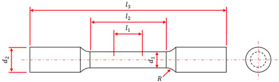
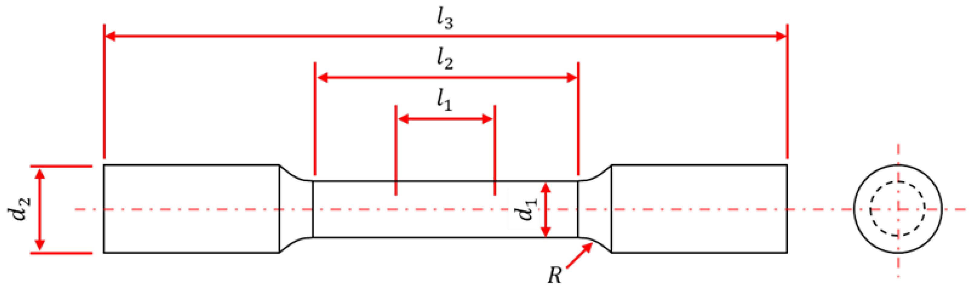
The 10705MBU stainless steel for turbine blades was used for the test. According to the ASTM E8/E8M standard, specimens with circular cross-sections were used to define the universal physical properties for the plastic processing of the material, as shown in Figure 1. Furthermore, the dimensions of the specimens are listed in Table 1.

Figure 1. Schematic of the ASTM E8/E8M tensile specimen.

Table 1. Dimensions of the specimens.

Symbol	Description	Value
l1	Gauge length	62.5 mm
l2	Length of reduced section	75 mm
l3	Total length	145 mm
d1	Diameter of reduced section	12.5 mm
d2	Diameter of grip	12.5 mm
R	Radius of fillet	10 mm

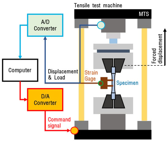
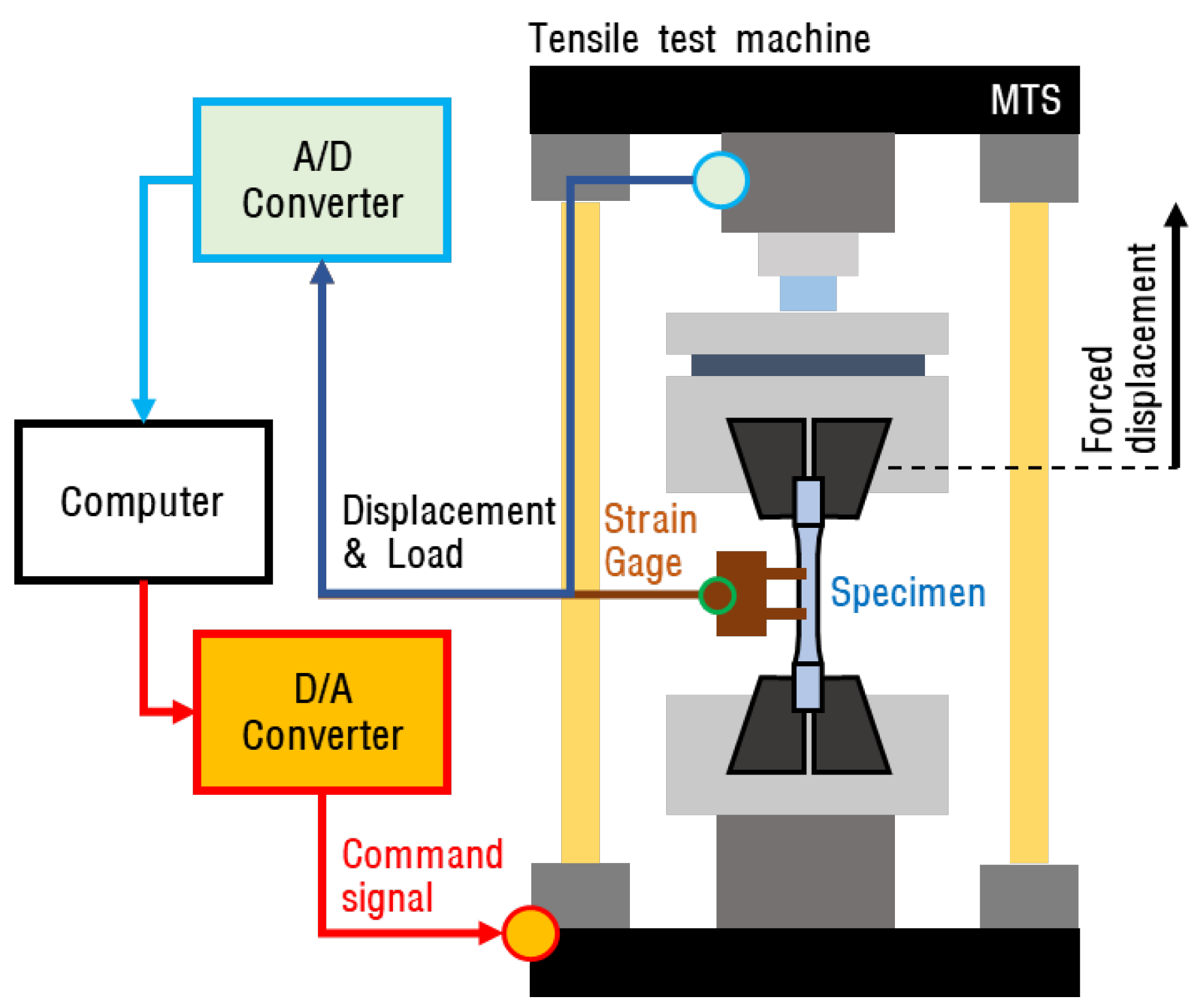
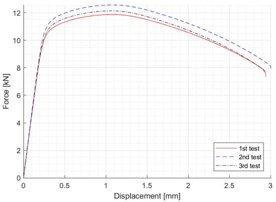
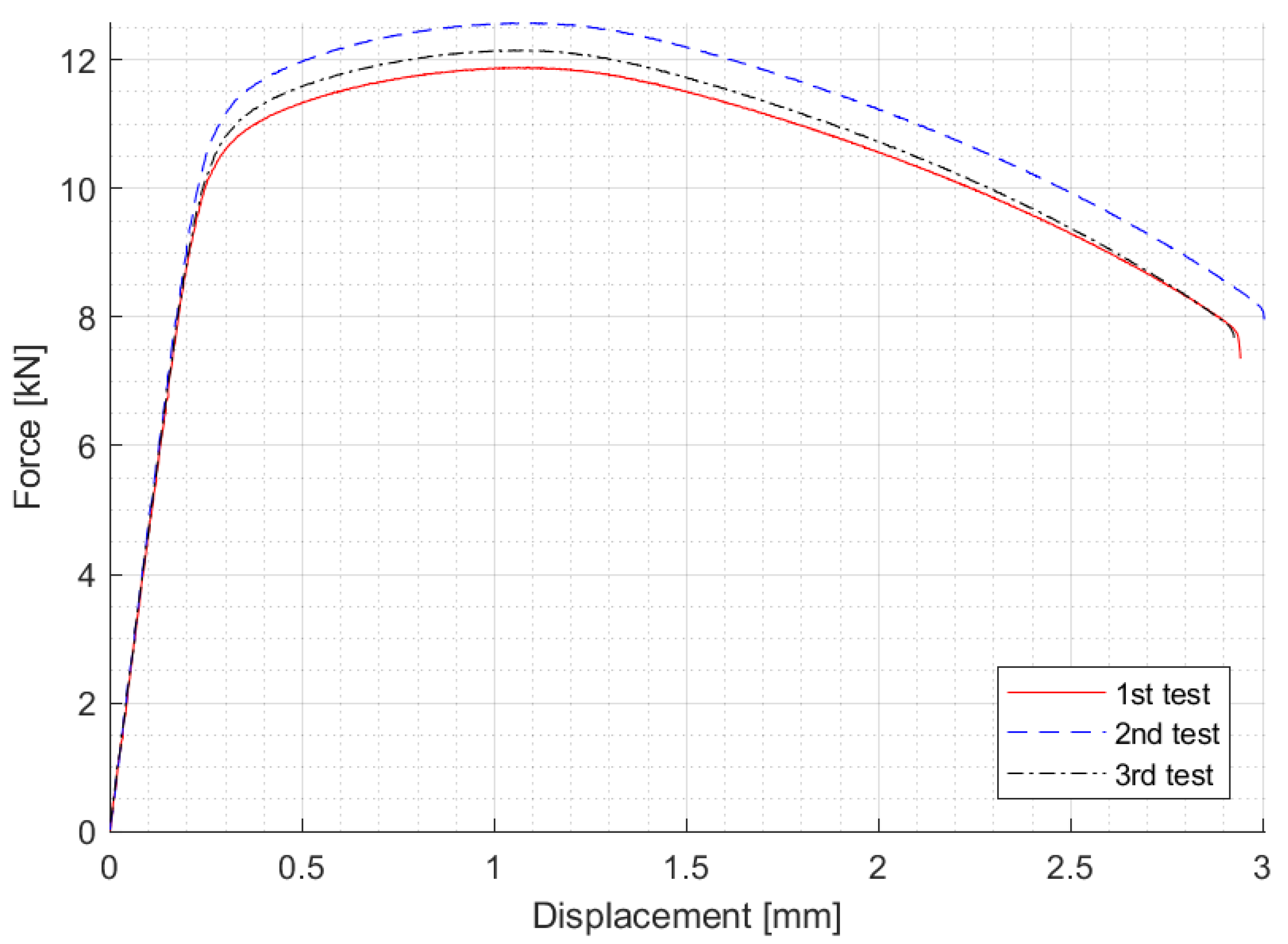
A conceptual diagram of the ASTM E8/E8M tensile test is presented in Figure 2. The tensile tester induced specimen deformation by causing a forced displacement. In this process, the load applied to the tensile tester (MTS 810 Universal Testing Machine) and the displacement measured using a strain gauge were recorded using a computer. The displacement and load data were stored in a two-dimensional matrix and displayed in a graph, as shown in Figure 3.

Figure 2. Schematic of the ASTM E8/E8M tensile test.

Figure 3. Results of the tensile test (ASTM E8/E8M).

2.2. Initialization of Constitutive Model Parameters for True Stress–Strain Curve

The load–displacement data, which are the result of the tensile test, can be expressed by the constitutive model for engineering stress–strain. The engineering stress–strain relationship is linear. The engineering strain can be expressed by the relationship between the initial gauge length and the strain amount of the gauge length, and is as shown in Equation (1). The engineering stress can be expressed by the relationship between the elastic modulus and the engineering strain, and can be expressed by the relationship between the load and the central cross-sectional area, as shown in Equation (2). When a material is subjected to yield stress, the stress–strain relation is transformed into a non-linear property, which is shown in Equations (3) and (4). The constitutive model for true stress–strain is an equation to briefly explain this non-linear behavior. Constitutive models for stress–strain are equations that can easily describe such nonlinear behaviors.

$$\begin{array}{cc}\hfill {\sigma }_e& =E{\epsilon }_e\hfill \\ & =\frac{F}{A}\hfill \end{array}$$

(1)

$$\begin{array}{cc}\hfill {\sigma }_e& =E{\epsilon }_e\hfill \\ & =\frac{F}{A}\hfill \end{array}$$

(2)

$${\epsilon }_t=\ln \left(1+{\epsilon }_e\right)$$

(3)

$${\sigma }_t={\sigma }_y+K{({\epsilon }_y+{\epsilon }_t)}^n$$

(4)

In these equations, E denotes Young’s modulus, δ is the displacement, L is the gauge length, ${\sigma }_e$ is the engineering stress, ${\epsilon }_e$ is the engineering strain, F is the external force, ${\sigma }_e$ is the central cross-sectional area of the specimen, ${\epsilon }_t$ is the true strain, ${\sigma }_y$ is the yield stress, K is the plastic strength coefficient, n is the work-hardening parameter, and ${\epsilon }_y$ is the yield strain. Equations (1) and (2) represent the material’s elasticity ($0\le \epsilon \le {\epsilon }_y$). Equations (3) and (4) represent the material’s plastic area as a polynomial function and Gosh models, respectively, where (${\epsilon }_y\le \epsilon$). However, various constitutive models must be established because each material has a different curve characteristic for the plastic area.

Table 2 lists the names, equations, and the number of parameters of the true stress constitutive models for the plastic area. Among the presented constitutive models, only the engineering dataset is an engineering stress–strain model, and the rest (Models 1–3) are true stress–strain models. In these models, ${\sigma }_s$ is the saturation stress, ${\sigma }_y$ is the yield stress, ${\epsilon }_y$ is the yield strain, b and p are material properties, n is the work-hardening parameter, K is the plastic strength coefficient, and α is the combination factor. The true stress–strain constitutive model for metals is distinguished by the curved shape of the polynomial (Model 1) [44,45,46] and exponential models (Model 2) [47,48,49] listed in Table 2. If the constitutive model cannot sufficiently express the nonlinear behaviors of the specimen, combination functions (Model 3) [29,42] can be considered. The combination function uses α to combine the properties of the power and exponential functions. In addition, various component equations were used to express the nonlinear properties.

Table 2. Various constitutive model details for FE simulation.

No.	Description	Constitutive Models (εy ≤ ε)	Number of Variables
-	Engineering data	${\sigma }_e={\sigma }_e$	-
-	ASTM E646	${\sigma }_t={\sigma }_e\left(1+{\epsilon }_t\right)$	-
1	Gosh	${\sigma }_g={\sigma }_y+K{({\epsilon }_y+{\epsilon }_t)}^n$	4
2	Hockett–Sherby	${\sigma }_{hs}={\sigma }_s-\left({\sigma }_s-{\sigma }_y\right)\times \exp \left(-b{\epsilon }_t{}^p\right)$	4
3	Gosh and Hockett–Sherby	${\sigma }_{gh}=\alpha {\sigma }_{go}+\left(1-\alpha \right){\sigma }_{hs}$	8

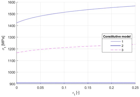
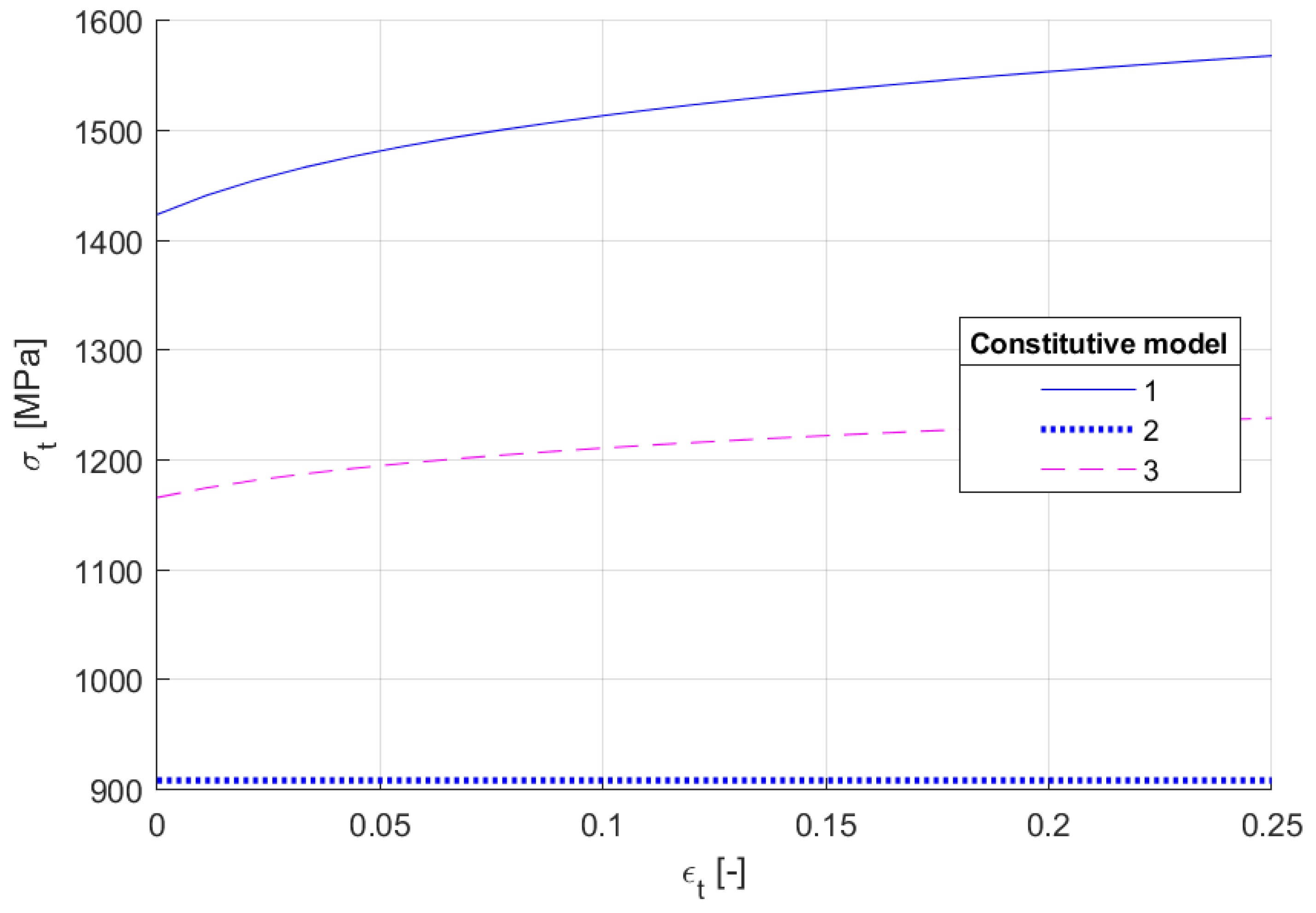
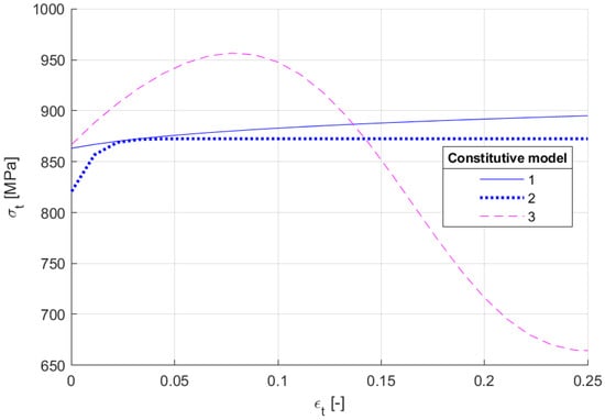
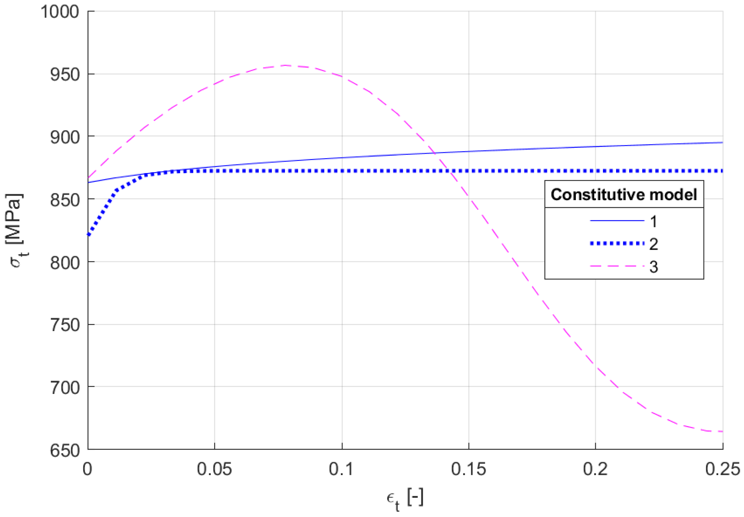
The parameters of the constitutive models listed in Table 2 were initialized using the numerical linear algebra method proposed by the ASTM E646 standard, and the results are shown in Figure 4. The X-axis and Y-axis in Figure 4 represent the engineering strain and true stress values, respectively. Model 1 presents the engineering stress–strain values of the experimental data. The σ_y, ε_y, and σ_s were initialized using E and slope values between the data. Furthermore, the b, n, and K were initialized using the numerical linear algebra method based on the ASTM E646 standard, and α was initialized to 1.0 for Model 1, 0.0 for Model 2, and 0.5 for Model 3. The initialized parameters were commonly applied to every constitutive model. However, as indicated in Figure 4, the characteristics of the true stress–strain curve were significantly different from Model 1. This result implies that the parameters must be initialized differently depending on the constitutive model.

Figure 4. Constitutive model properties initialization using the ASTM E646 standard.

2.3. CFT Method for Constitutive Model of the True Stress–Strain Curve

As shown in Figure 4, the constitutive model properties initialized by the ASTM E646 standard did not correctly represent the actual physical phenomenon. This error can result in an error in the FE simulation and the load of the inverse method. Therefore, individual curve fitting of the constitutive model properties is required. The result of modifying a once-initialized parameter using MATLAB CFT is shown in Figure 5. Notably, the parameter initialization method reduced the difference between the experimental data and the constitutive model properties. This finding reveals that the constitutive model properties using the power and exponential functions cannot represent the actual physical phenomena. Furthermore, it can be observed that the combination function with several parameters exhibited accurate nonlinear characteristics.

Figure 5. Constitutive model properties initialization using ASTM E646 and MATLAB CFT.

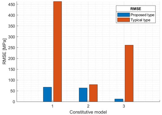
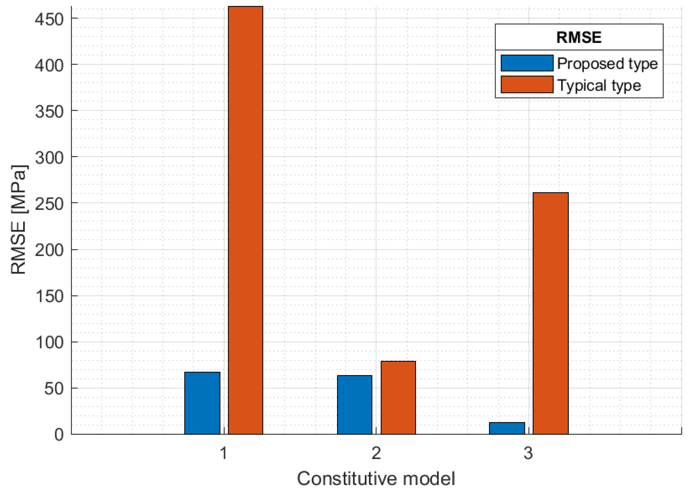
The difference between the experimental data and the constitutive model can be observed qualitatively in Figure 4 and Figure 5; RMSE is used to compare the differences quantitatively. Figure 4 and Figure 5 show the actual strain assuming zero yield strain. This method was later used to apply to material cards for FE simulations. The results of the quantitative comparison and analysis of the two datasets are shown in Figure 6. The X-axis and Y-axis in Figure 6 represent the constitutive model number and the RMSE value (between the constitutive model properties and experimental data), respectively. The solid red line indicates the RMSE value of the once-initialized constitutive model, and the dotted line indicates the RMSE value of the constitutive model to which the MATLAB CFT was applied. It may be observed that, except for Models 1 and 2 with no parameters, the proposed method using MATLAB CFT obtained an RMSE reduction effect for every constitutive model. This can be seen as a process of giving an initial value of a parameter rather than a specific result. Since the target of curve fitting is the engineering stress–strain, it is difficult to discuss the accuracy of Figure 6. The parameter initialization of the pretreatment step plays a role in determining the curve characteristics represented by the constitutive model. The accuracy of the configuration model can later be increased in the inverse method. However, if the typical method (Figure 4) is to be used, both the characteristics and accuracy of the curve should be determined with the inverse method.

Figure 6. Quantitative comparison between the typical and proposed methods.

3. FE Simulation

FE simulations can define material properties with the constitutive model of true stress–strain. Then, the engineering stress–strain can be derived as the FE simulation result. The FE simulation results and experimental data are appropriate for comparison because they are both engineering stress–strain data [50].

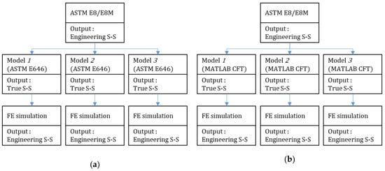
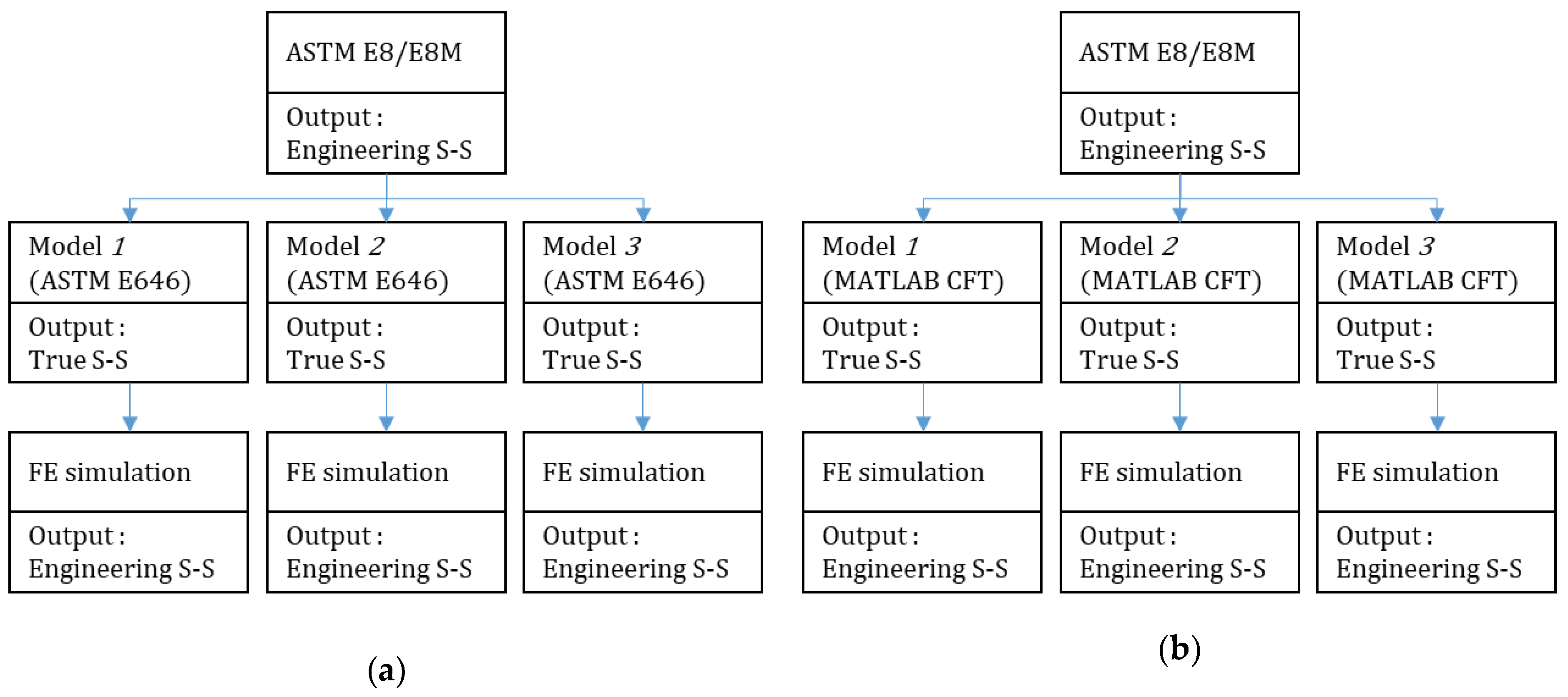
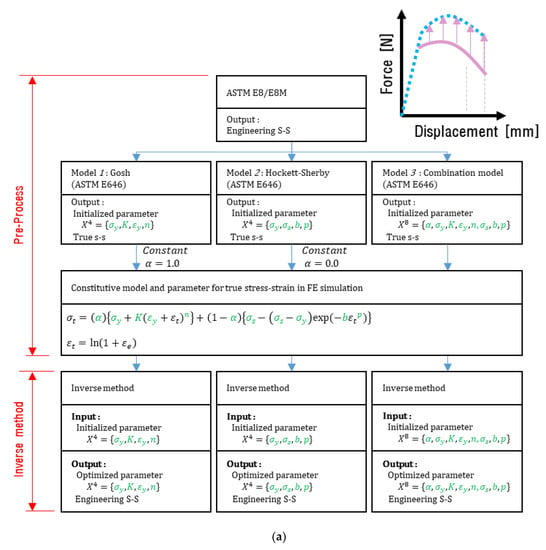
In the pre-processing stage, the typical method only used the ASTM E646 standard, whereas the proposed method used the ASTM E646 standard and MATLAB CFT. To validate the proposed method, FE simulation was performed six times, as each constitutive model and pre-processing method was performed once. Figure 7 presents the procedures for the typical and proposed methods. The constitutive models used in the FE simulation are listed in Table 2. The parameter values applied to the constitutive model are the same as those in Table 3. FE simulation was performed using the universal FE code LS-Dyna/Explicit, and the difference between the analysis results and experimental data is represented using the RMSE values.

Figure 7. FE simulation procedures: (a) method that initializes the parameter once; (b) method that applies CFT.

Table 3. Definition of parameter for constitutive model.

Symbol	Unit	ASTM & Experience Value			Matlab CFT
		Model 1	Model 2	Model 3	Model 1	Model 2	Model 3
εy	mm/mm	0.018	0.018	0.018	0.018	0.018	0.018
σy	MPa	208	208	208	735.708	735.708	735.708
σs	MPa	908	908	908	-	872.42	1249.410
b	-	2.9725	2.9725	2.9725	-	600.00	12.000
p	-	1	1	1	-	1.575	0.905
n	-	−0.0063	−0.0063	−0.0063	0.120	-	0.596
K	MPa	938	938	938	187.766	-	1983.170
$\alpha$	-	1.0	0.0	0.5	-	-	2.633

3.1. Material Model

The material card of LS-Dyna/Explicit for plastic deformation simulation requires true stress–strain curve data, which can be applied through the pre-processing. The properties of the constitutive models were applied using the MAT 24 materials card supported by LS-Dyna.

3.2. FE Modeling

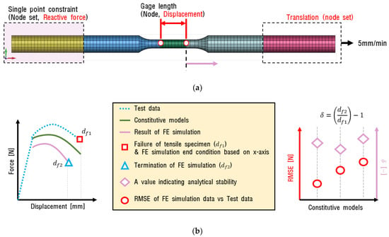
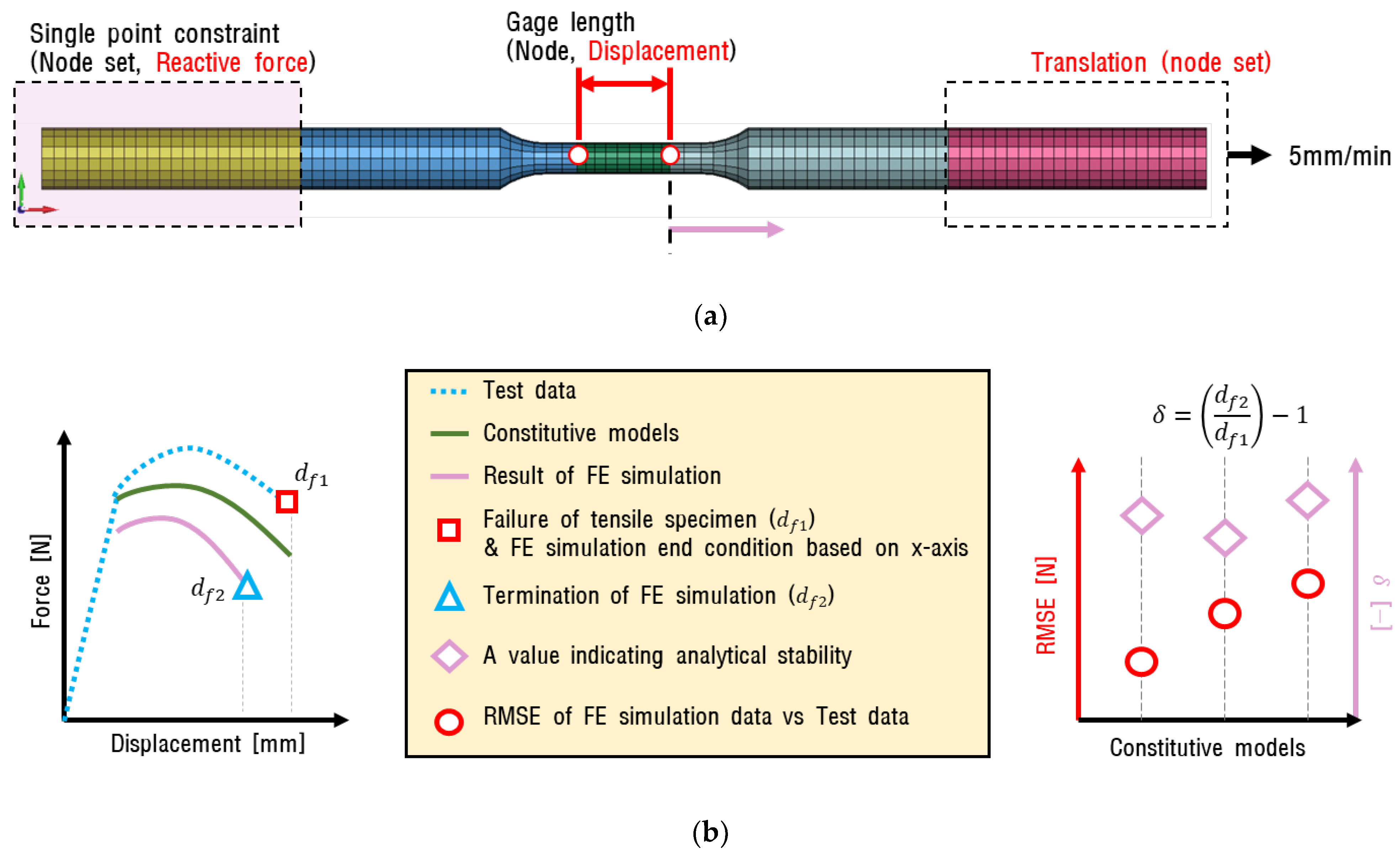
The FE model and boundary conditions for the FE simulation are shown in Figure 8a. The elements were longitudinally divided into 99 equal lengths and constituted 32 elements based on the cross-section. The average length of the elements was 1.5 mm, and they were modeled in a hexahedron shape with eight integration points. To simulate the actual test environment, the fixed and forced displacement conditions were applied to the left and right sides of the model, respectively. The displacement of the central part and the repulsion force of the fixed part were observed during the analysis. Except for the constitutive model properties, the simulation conditions were identical. The maximum displacement of the experimental data was applied as the termination condition for the FE simulation and was performed from zeros until the termination condition was satisfied. These conditions are shown in Figure 8b. In this process, the termination condition was satisfied differently depending on the properties of the constitutive model, and it was difficult to predict the termination time. While extracting data at regular time intervals, it was found that the error for the maximum deformation of the FE simulation was within 5%.

Figure 8. FE model of tensile specimen: (a) Finite element model and boundary condition; (b) Concept of FE simulation results.

3.3. Results of FE Simulation

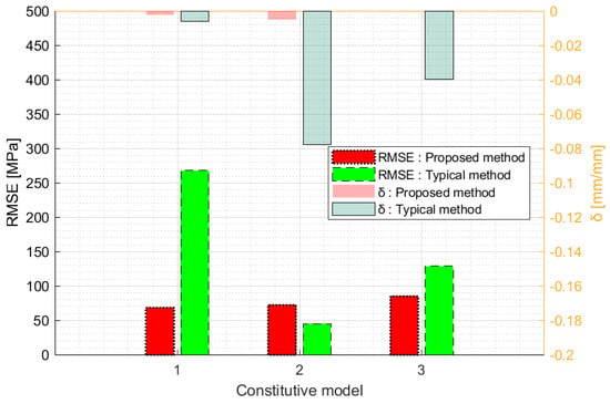
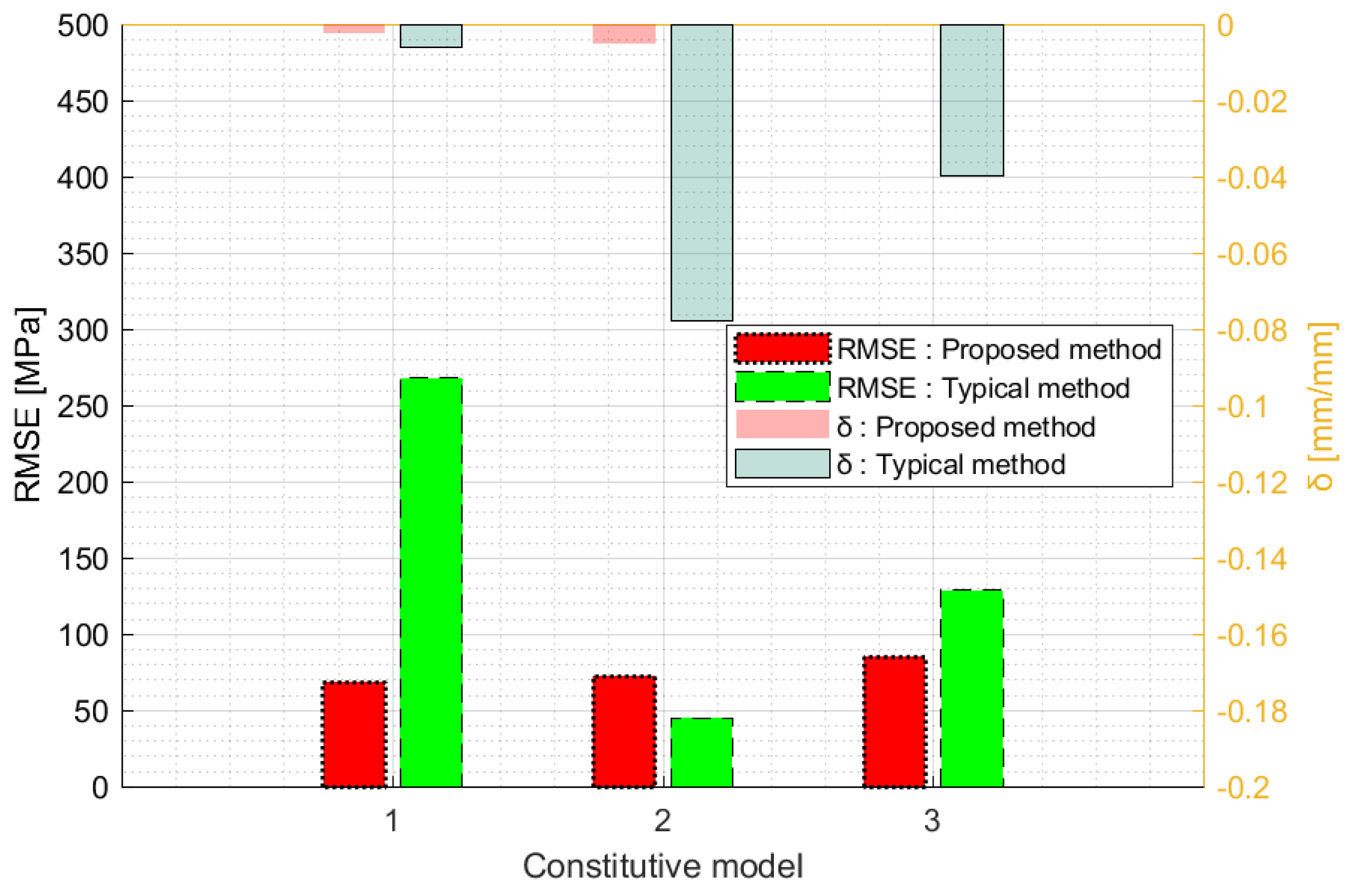
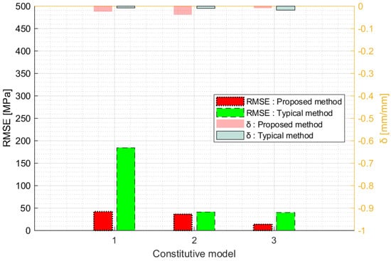
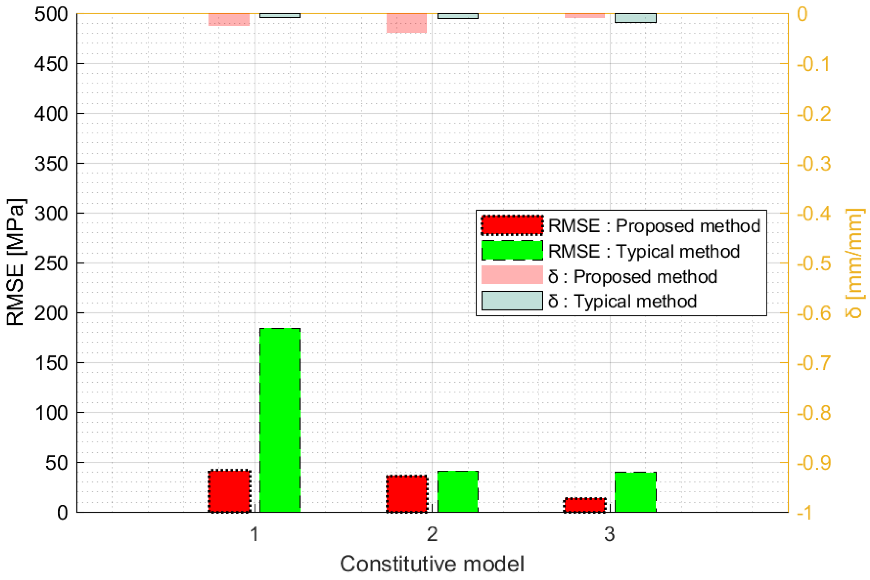
The RMSE values of the FE simulation results and test results were compared, as shown in Figure 9. In addition, the criterion for verifying the normal performance of the analysis is represented by $\delta$. $\delta$ is an index indicating whether the analysis was performed normally by dividing the maximum value ($d_{f1}$) of the tensile test displacement by the maximum value ($d_{f2}$) of the FE simulation displacement. As a result of performing FE simulation using the proposed method, the RMSE value decreased in every constitutive model except Model 2. Furthermore, the $\delta$ value of the proposed method was higher than that of the typical method. A value of $\delta$ closer to one indicates a more stable analysis result.

Figure 9. Comparison between RMSE values of FE simulation results and test results.

4. Inverse Method

4.1. Metamodel-Based Simulation Optimization

The metamodel-based optimization technique is an optimization theory that reduces the cost of numerous repeated failures. This optimization theory repeatedly carries out a sequence of operations consisting of setting the parameter range, performing the design of the experiment, generating the response surface, analyzing the response surface, and conducting a convergence test. A metamodel represents the correlation between the parameter change and response. The inverse method can be considered as a metamodel-based optimization technique that uses the properties of the metamodels for FE simulation and the RMSE response surface; it is also referred to as FEMU.

4.2. Inverse Method Using Metamodel-Based Simulation Optimization

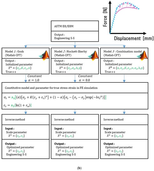
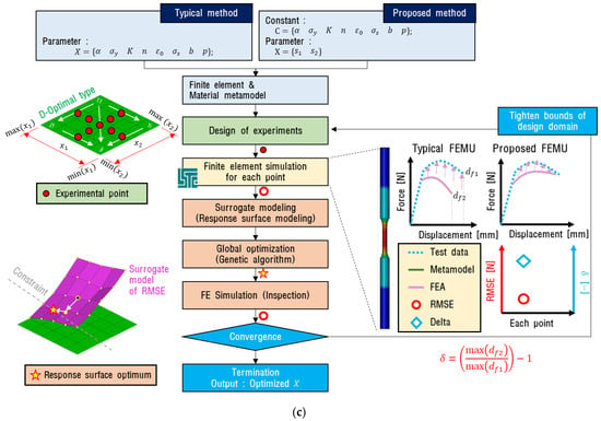
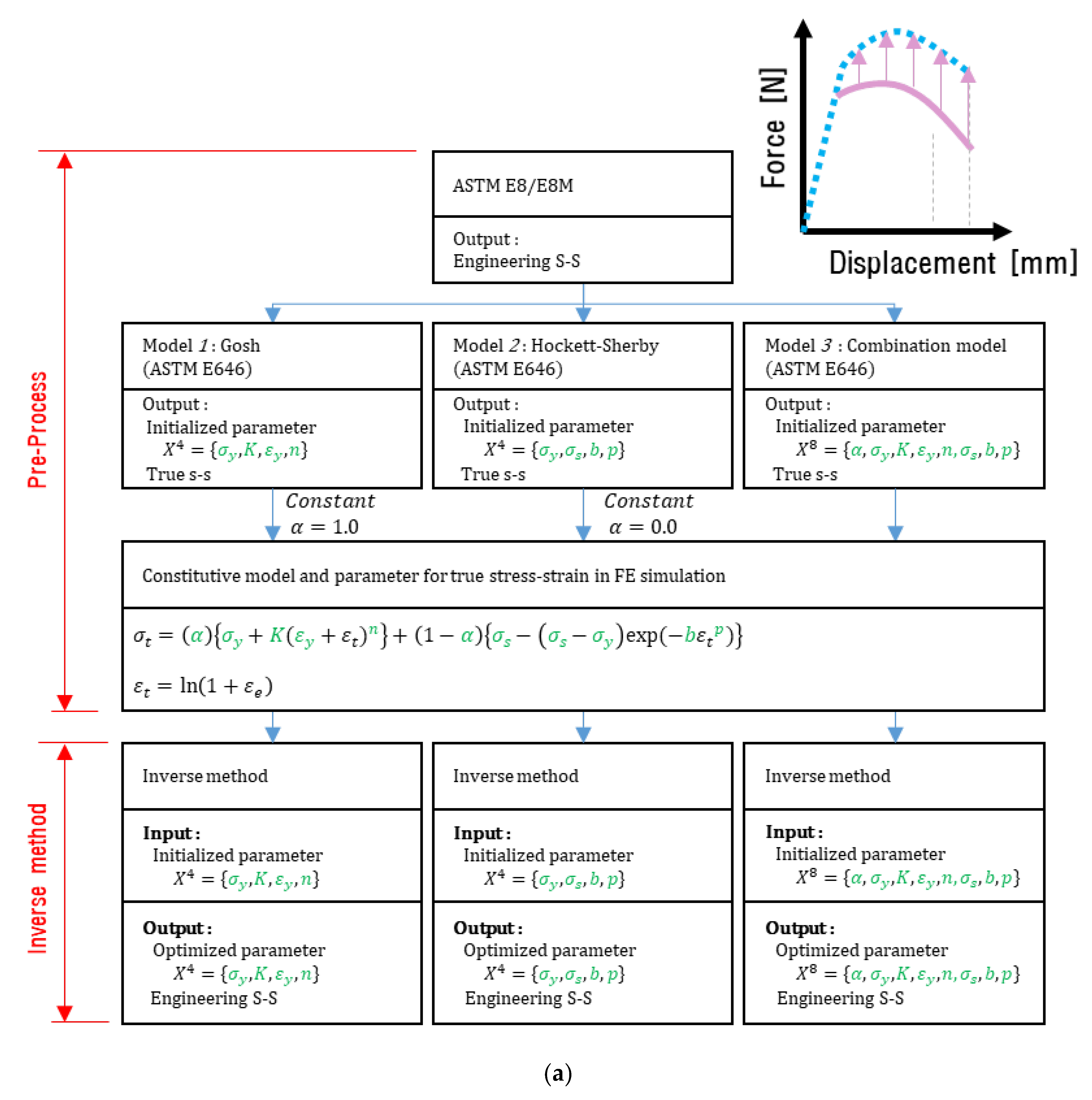
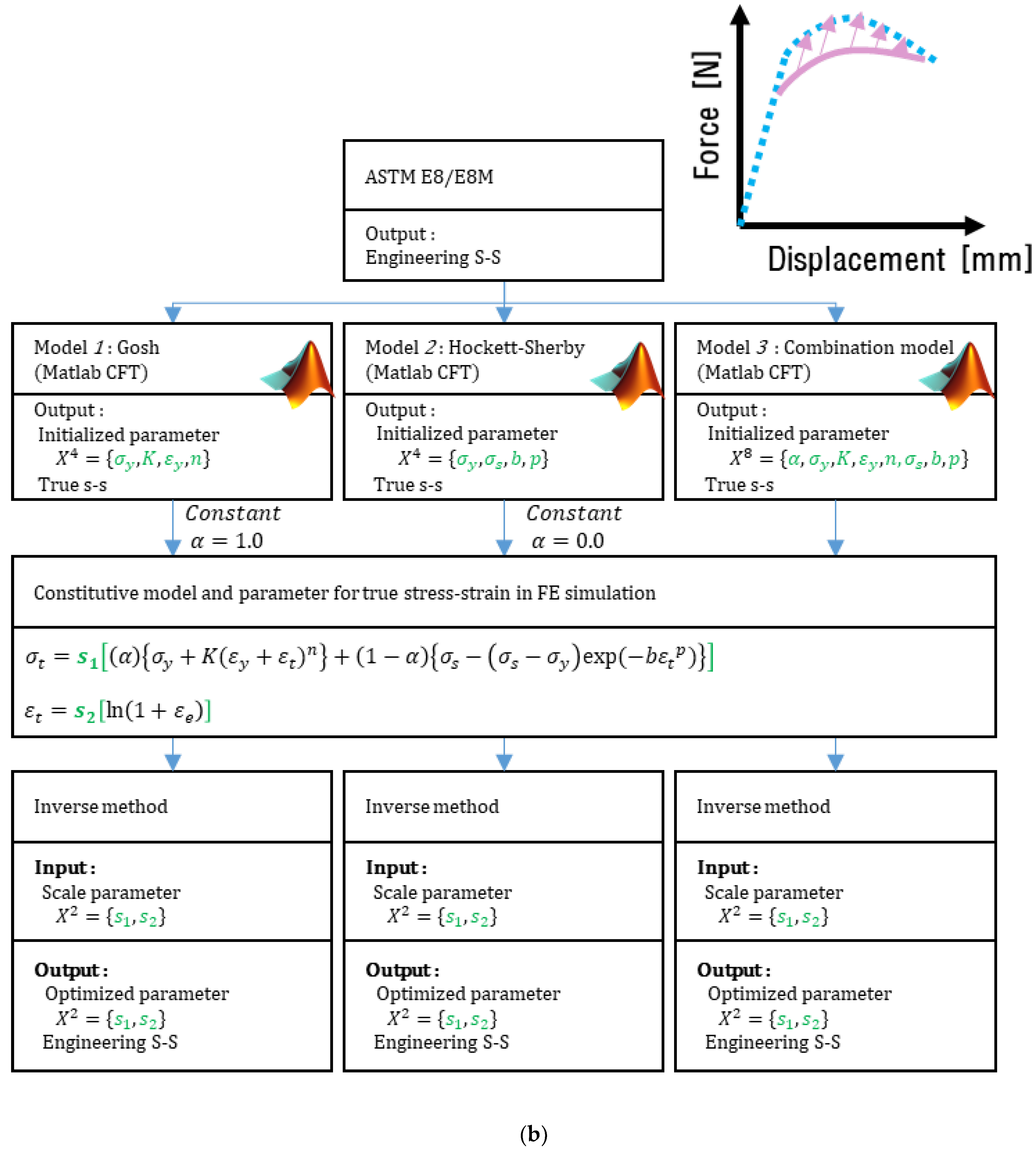
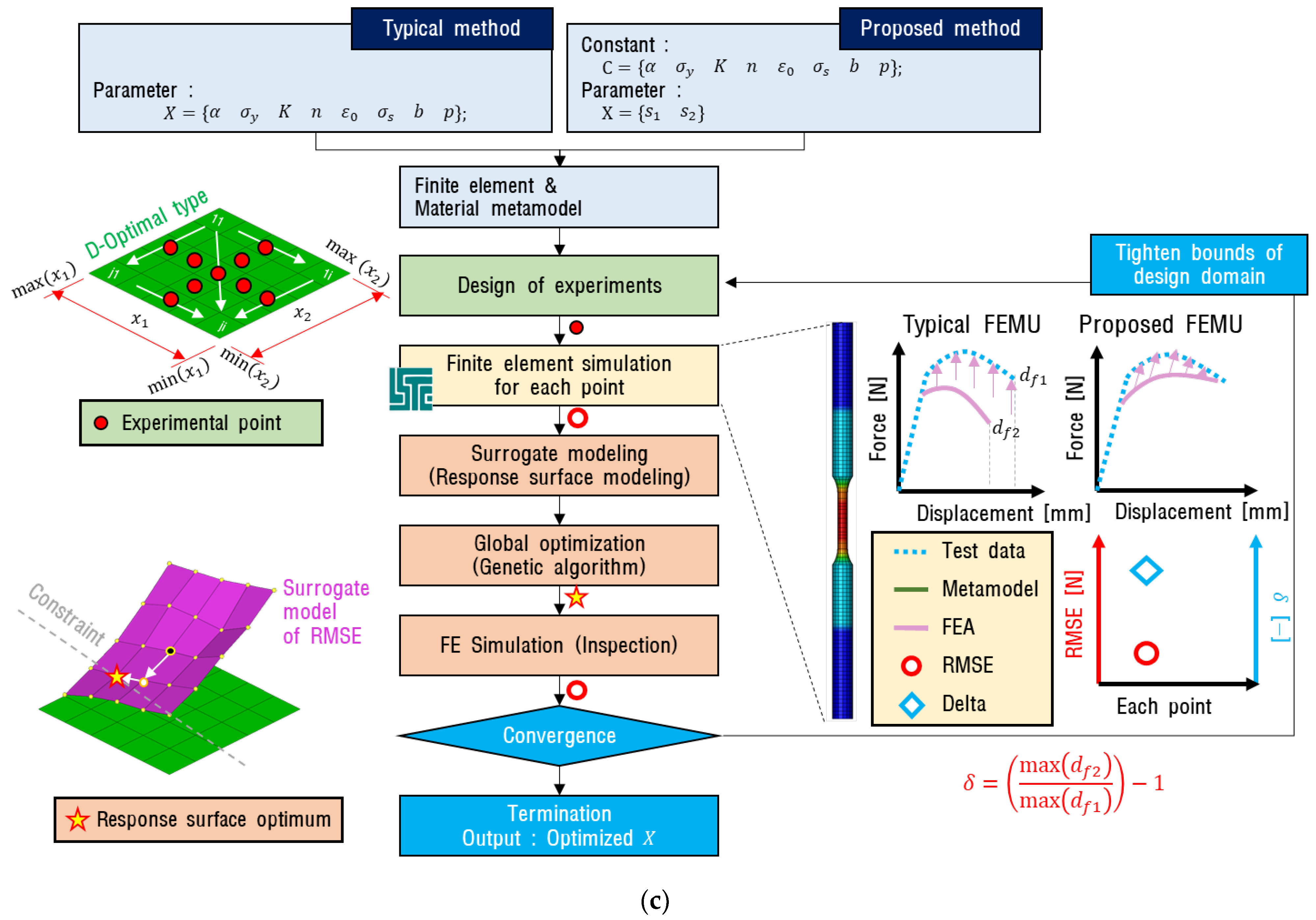
Figure 10 shows the relationship between the pre-processing step and the inverse method step. Equation (5) shows the most complex form (Model 3) of the configuration model by pre-process. Equation (6) shows Model 3 with Matlab CFT with the scale factor (s₁) applied. Equation (7) shows an application example of the scale factor (s₂) applied to the true strain value.

$${\sigma }_t=\left(\alpha \right)\left\{{\sigma }_y+K{({\epsilon }_y+{\epsilon }_t)}^n\right\}+\left(1-\alpha \right)\left\{{\sigma }_s-\left({\sigma }_s-{\sigma }_y\right)exp\left(-b{\epsilon }_t{}^p\right)\right\}$$

(5)

$${\sigma }_t={\mathit{s}}_{\mathbf{1}}\left[\left(\alpha \right)\left\{{\sigma }_y+K{({\epsilon }_y+{\epsilon }_t)}^n\right\}+\left(1-\alpha \right)\left\{{\sigma }_s-\left({\sigma }_s-{\sigma }_y\right)exp\left(-b{\epsilon }_t{}^p\right)\right\}\right]$$

(6)

$${\epsilon }_t={\mathit{s}}_{\mathbf{2}}\left[\ln \left(1+{\epsilon }_e\right)\right]$$

(7)

Figure 10. Inverse method procedure: (a) Typical method (metamodel-based simulation optimization with one-time initialization of variables); (b) Proposed method (metamodel-based simulation optimization using CFT); (c) Concept diagram of inverse method procedure.

As shown in Figure 10, constitutive Models 1, 2, and 3 were used for both the typical method and the proposed method.

In the pre-processing step, a tensile test was performed, and the configuration model was initialized via the load–displacement curve. In addition, the range of parameters was updated based on the RMSE value in the inverse method process. The D-Optimal method was used for the experiment design, which is advantageous for generating a regression equation-based response surface model [51,52]. The FE simulation was performed repeatedly by updating the parameters using the design of the experiment. In this process, the quantitative error of the FE simulation was calculated using RMSE, and the correlation between the parameter changes and RMSE was approximated by the response surface, which is composed of a linear equation. When an error occurred, it was composed of a quadratic polynomial equation. This nonlinearity of the response surface influenced the design of the experiment and the number of FE analysis iterations performed.

Figure 10a shows the flow of a typical method. In the pre-processing stage, only the parameters were initialized using the ASTM E646 standard, and for the inverse method, the parameter set X was used for the design of the experiment as they were. Figure 10b shows the flow of the proposed method. During the pre-processing, the parameters were initialized using the ASTM E646 standard and MATLAB CFT, and the scale parameters of the stress and strain axes for the true stress–strain curve were used as the set of inverse method parameters X.

$$v=\left\{q\left(k_{max}-1\right)\right\}+1$$

(8)

The total iteration count (v) of the FE simulation required by the inverse method can be calculated using Equation (8) (da Fonseca et al., 2005). Here, k denotes the iteration, and q is the required iteration count of the FE simulation per iteration. The value of q may vary according to the number of parameters, the curvature of the response surface, and the theory of the experiment design. In the last iteration of the inverse method, only one FE simulation was performed for verification. A genetic algorithm was used to analyze the response surface model and was used to derive the lowest RMSE within the range of the response surface and the parameter value that it satisfied. Convergence was determined through changes in the RMSE values and parameters. If the RMSE values from each FE simulation were larger than 0.01, the parameter range was adjusted around the optimal point, and the experimental plan was recreated. The inverse method was set to end when the average change in RMSE was less than 0.01%, the amount of average change in the parameter was less than 0.01, and the number of iterations was 50.

4.3. Results of the Inverse Method

Figure 11 shows the differences in the inverse method between the typical and proposed methods based on the RMSE value. The effect of the inverse method can be observed by comparing the RMSE values in Figure 9 and Figure 11. The polynomial model (Model 1) and exponential model (Model 2) showed relatively large errors, and the combination function (Model 3) showed the lowest RMSE value. Then, the RMSE value of the proposed method was derived to be relatively low compared to the typical method.

Figure 11. Comparison between the inverse method of the typical and proposed methods based on the RMSE values.

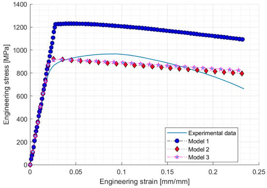
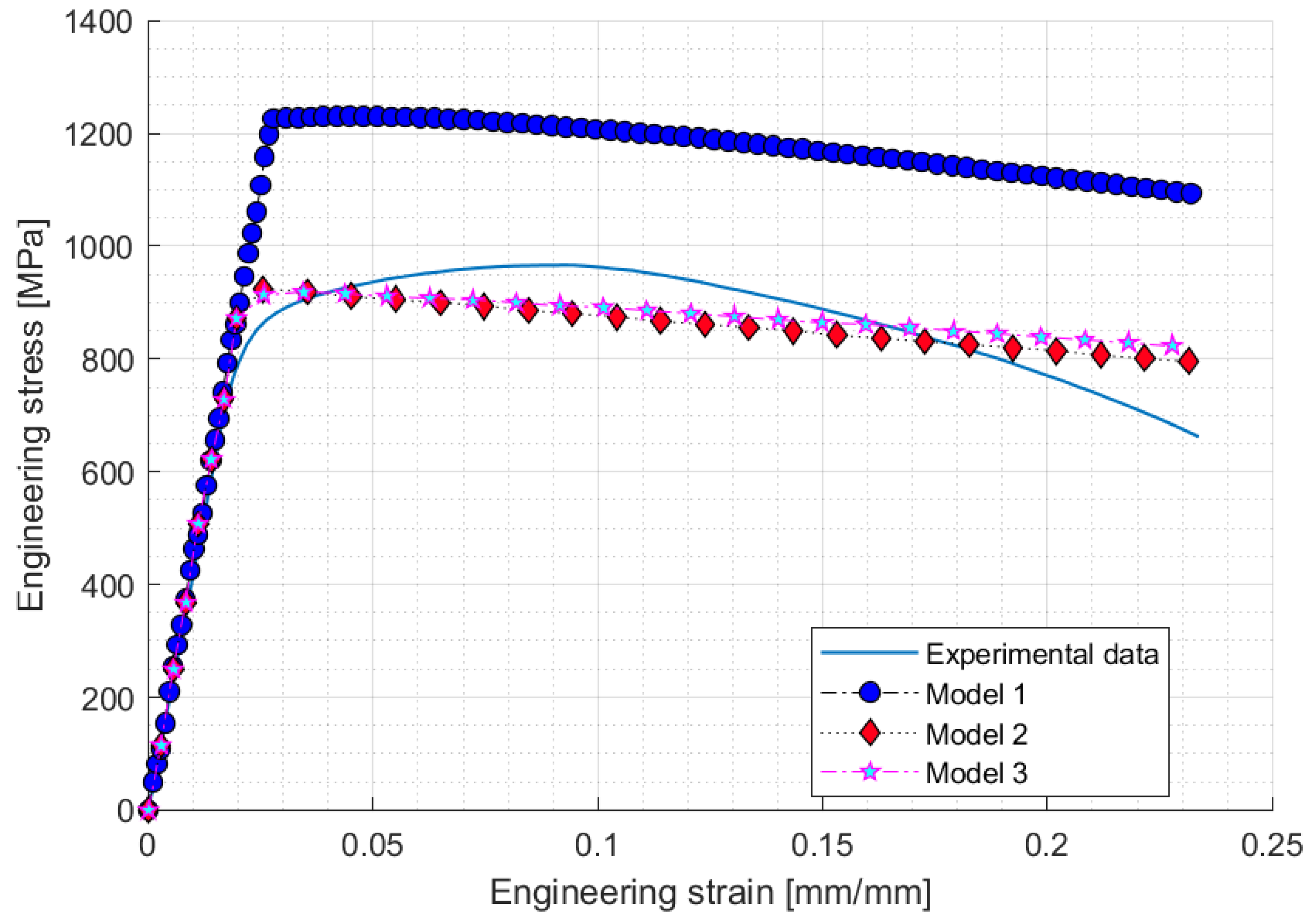
Figure 12 shows the engineering stress–strain curves derived using the typical method. There was a difference in expressing the test data depending on the curve characteristics of the constitutive model. Since the objective function of the typical method sets only RMSE minimization, it is evident that the characteristics of the curve appear linearly, and the polynomial function (Model 1) did not approach the reference data. From these results, it is apparent that the factors were set inappropriately at the initialization stage. Inappropriate results, such as those shown in Figure 12, depend on changes in test data, MBSO algorithms, objective functions, and other factors. However, Figure 12 shows the results of using the MBSO algorithm used in this study.

Figure 12. Inverse method results for typical method.

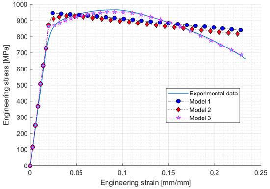
Figure 13 shows the analysis results obtained by applying the proposed method to each constitutive model. The polynomial function (Model 1) and exponential function (Model 2) show a linear trend, similar to the results of the structural method. This result can be derived from the low RMSE value presented in Figure 11. The combination function (Model 3) of the proposed method showed the same results as the test data because the configuration model is complicated. It is observed that the result of the inversion method does not appear linear because the curve characteristics determined in the previous step are maintained. The results of the proposed methods are not always perfect, as in Model 1 and Model 2. However, despite being a suitable configuration model, the structural method did not demonstrate a good performance. Subjectively, the reason these results appear is that the inverse method attempts to curve fit both curve characteristics and curve accuracy.

Figure 13. Inverse method results for the proposed method.

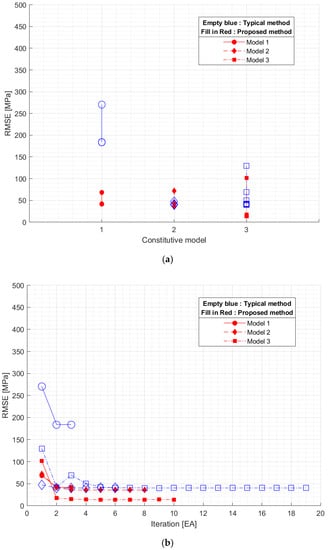
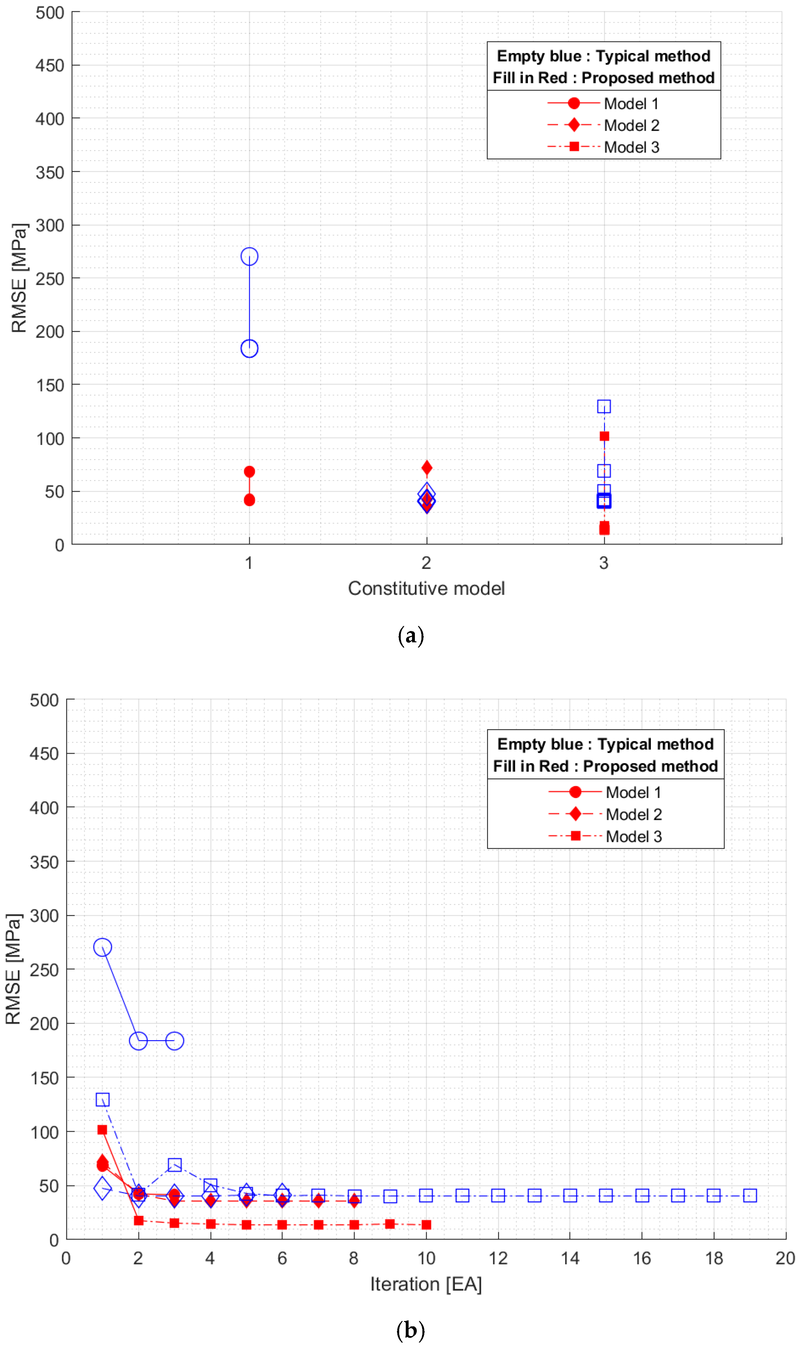
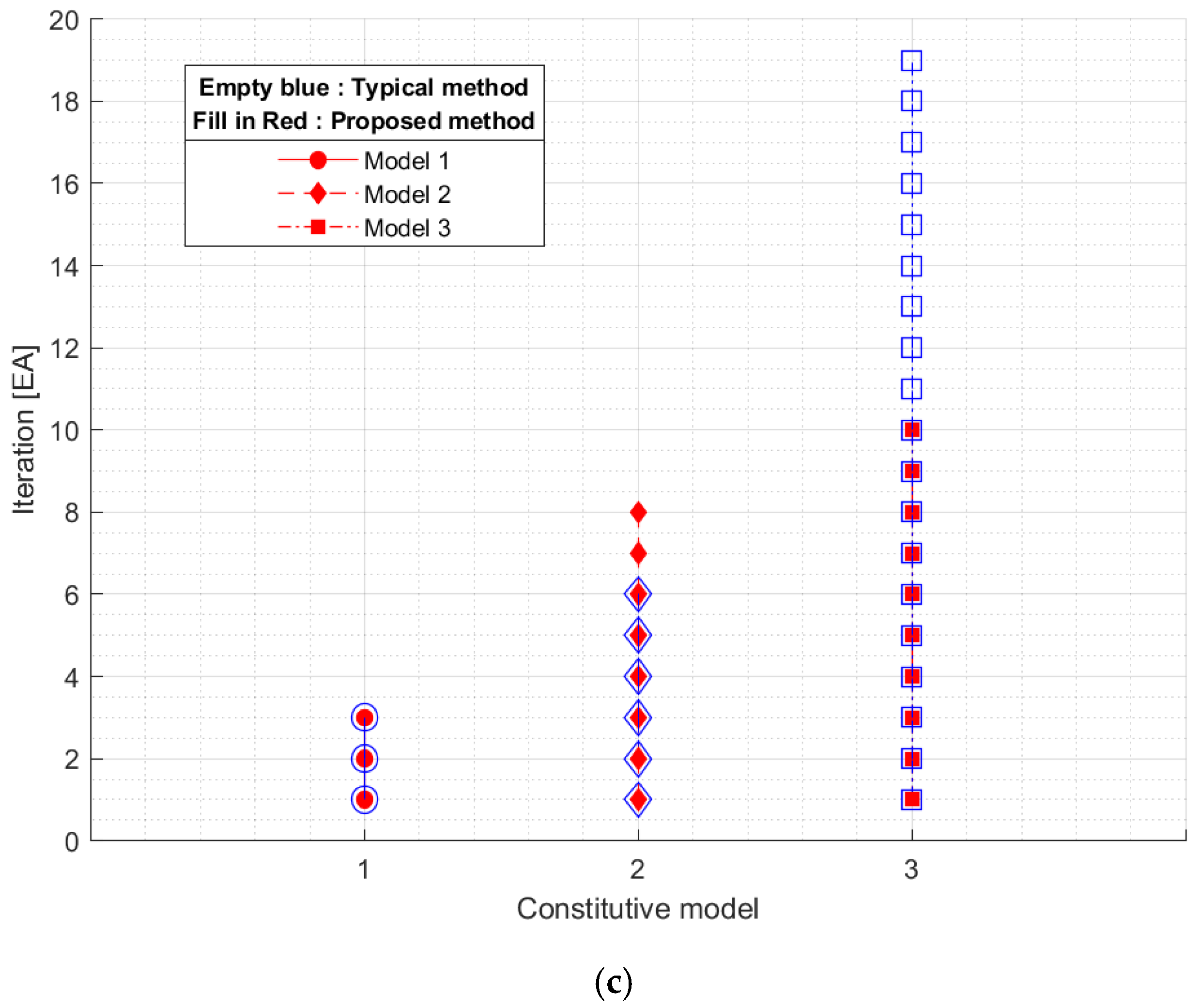
Figure 14 shows the RMSE and iterations for Models 1, 2, and 3. As shown in Figure 14a, the proposed method showed a relatively low RMSE value compared with the typical method. Figure 14b shows how the RMSE value changed owing to the iteration of the inverse method. Model 1 had no difference in iteration. Model 2 had more iterations of the proposed method. There were more iterations of the typical method for Model 3. This trend can be reliably compared in Figure 14c.

Figure 14. Convergence process of inverse method. (a) Constitutive model vs RMSE; (b) Iteration vs RMSE; (c) Constitutive model vs Iteration.

Table 4 shows the parameter values derived from the inverse method. Table 5 shows the number of variables used in the inverse method, maximum number of iterations until convergence, number of SE simulations required by the design of the experiment, sum of FE simulations until convergence, and convergence result represented by RMSE. Table 5 has the total number of interpretations based on Equation (8). The proposed method saved 1.4 times more resources in Model 1 and 5.3 times more in Model 3.

Table 4. Definition of parameter for constitutive model.

Symbol	Unit	ASTM & Experience Value			Matlab CFT
		Model 1	Model 2	Model 3	Model 1	Model 2	Model 3
εy	mm/mm	0.018	0.018	0.018	0.018	0.018	0.018
σy	MPa	735.708	735.708	735.708	735.708	735.708	735.708
σs	MPa	-	966.129	831.348	-	872.42	1249.410
b	-	-	33.005	28.754	-	600.00	12.000
p	-	-	0.0782	0.094	-	1.575	0.905
n	-	0.108	-	0.083	0.120	-	0.596
K	MPa	751.1	-	855.197	187.766	-	1983.170
α	-	-	-	0.765	-	-	2.633
s1	-	-	-	-	1.142	1.133	1.094
s2	-	-	-	-	1.100	1.100	1.412

Table 5. Results of specification in inverse method (A: Typical method, B: Proposed method).

No.	Number of Variables in the Inverse Method [EA]		Maximum Iteration [EA]		Total Experiment Points [EA]		Converged RMSE [MPa]
	A	B	A	B	A	B	A	B
1	4	2	4	3	16	11	194.6	41.5
2	4	2	6	8	36	36	41.2	35.9
3	8	2	18	10	325	61	37.0	14.0

5. Conclusions

The proposed method is generally the adding of a scale factor to the constitutive model that represents the material characteristics. Using the scale factor as a parameter in the inverse method, as in the proposed method, greatly reduces the number of cases that need to be tried, thus improving optimization efficiency. To validate the proposed method, nonlinear prediction characteristics were compared by applying three constitutive models, two pre-processing methods, and two inverse methods.

The combination function that applied the proposed method could accurately predict the nonlinear characteristics with fewer iterations. However, when the stress–strain curve characteristics of the constitutive model are inadequate, the inverse method does not converge or leads to inaccurate results. Therefore, if an MBSO incompatibility in a multifactorial environment with scaling factors is to be solved, it may be better to set the constitutive model to the combination function.

It is predicted that initializing the combination constitutive model and setting the inverse method parameters by applying the proposed method will improve the efficiency and accuracy of nonlinear analyses performed for large deformations. To achieve more accurate results, it is recommended to acquire the test data as true stress–strain. The reference data of this study were engineering stress–strain, but it is considered that more accurate results than those from this study can be obtained by acquiring true stress–strain using the DIC technique and performing inverse method.

References

- Kim, J.H.; Serpantié, A.; Barlat, F.; Pierron, F.; Lee, M.G. Characterization of the Post-Necking Strain Hardening Behavior Using the Virtual Fields Method. Int. J. Solids Struct. 2013, 50, 3829–3842. [Google Scholar] [CrossRef] [Scilit]
- Niutta, C.B.; Tridello, A.; Ciardiello, R.; Belingardi, G.; Paolino, D.S. Assessment of Residual Elastic Properties of a Damaged Composite Plate with Combined Damage Index and Finite Element Methods. Appl. Sci. 2019, 9, 2579. [Google Scholar] [CrossRef] [Scilit]
- Mazzon, E.; Habas-Ulloa, A.; Habas, J.P. Lightweight Rigid Foams from Highly Reactive Epoxy Resins Derived from Vegetable Oil for Automotive Applications. Eur. Polym. J. 2015, 68, 546–557. [Google Scholar] [CrossRef] [Scilit]
- Joun, M.S.; Eom, J.G.; Lee, M.C. A New Method for Acquiring True Stress-Strain Curves over a Large Range of Strains Using a Tensile Test and Finite Element Method. Mech. Mater. 2008, 40, 586–593. [Google Scholar] [CrossRef] [Scilit]
- Seon, G.; Makeev, A.; Schaefer, J.D.; Justusson, B. Measurement of Interlaminar Tensile Strength and Elastic Properties of Composites Using Open-Hole Compression Testing and Digital Image Correlation. Appl. Sci. 2019, 9, 2647. [Google Scholar] [CrossRef] [Scilit]
- Enami, K. The Effects of Compressive and Tensile Prestrain on Ductile Fracture Initiation in Steels. Eng. Fract. Mech. 2005, 72, 1089–1105. [Google Scholar] [CrossRef] [Scilit]
- ASTM E8/E8M -21 Standard Test Methods for Tension Testing of Metallic Materials; ASTM International: West Conshohocken, PA, USA, 2021. [CrossRef] [Scilit]
- Ling, Y. Uniaxial True Stress-Strain after Necking. AMP J. Technol. 1996, 5, 37–48. [Google Scholar]
- Cabezas, E.E.; Celentano, D.J. Experimental and Numerical Analysis of the Tensile Test Using Sheet Specimens. Finite Elem. Anal. Des. 2004, 40, 555–575. [Google Scholar] [CrossRef] [Scilit]
- Zhang, Z.L.; Hauge, M.; Ødegård, J.; Thaulow, C. Determining Material True Stress-Strain Curve from Tensile Specimens with Rectangular Cross-Section. Int. J. Solids Struct. 1999, 36, 3497–3516. [Google Scholar] [CrossRef] [Scilit]
- Tvergaard, V. Effect of Kinematic Hardening on Localized Necking in Biaxially Stretched Sheets. Int. J. Mech. Sci. 1978, 20, 651–658. [Google Scholar] [CrossRef] [Scilit]
- Needleman, A.; Tvergaard, V. Necking of Biaxially Stretched Elastic-Plastic Circular Plates. J. Mech. Phys. Solids 1977, 25, 159–183. [Google Scholar] [CrossRef] [Scilit]
- Tvergaard, V.; van der Giessen, E. Effect of Plastic Spin on Localization Predictions for a Porous Ductile Material. J. Mech. Phys. Solids 1991, 39, 763–781. [Google Scholar] [CrossRef] [Scilit]
- Dziallach, S.; Bleck, W.; Blumbach, M.; Hallfeldt, T. Sheet Metal Testing and Flow Curve Determination under Multiaxial Conditions. Adv. Eng. Mater. 2007, 9, 987–994. [Google Scholar] [CrossRef] [Scilit]
- Liu, X.; Ma, H.; Fan, F. Modified Johnson–Cook Model of SWRH82B Steel under Different Manufacturing and Cold-Drawing Conditions. J. Constr. Steel Res. 2021, 186, 106894. [Google Scholar] [CrossRef] [Scilit]
- Wang, Y.; Zeng, X.; Chen, H.; Yang, X.; Wang, F.; Zeng, L. Modified Johnson-Cook Constitutive Model of Metallic Materials under a Wide Range of Temperatures and Strain Rates. Results Phys. 2021, 27, 104498. [Google Scholar] [CrossRef] [Scilit]
- Qian, X.; Peng, X.; Song, Y.; Huang, J.; Wei, Y.; Liu, P.; Mao, X.; Zhang, J.; Wang, L. Dynamic Constitutive Relationship of CuCrZr Alloy Based on Johnson-Cook Model. Nucl. Mater. Energy 2020, 24, 100768. [Google Scholar] [CrossRef] [Scilit]
- Yue, N.; Li, L.; Morandi, A.; Zhao, Y. A Metamodel-Based Multi-Objective Optimization Method to Balance Thermal Comfort and Energy Efficiency in a Campus Gymnasium. Energy Build. 2021, 253, 111513. [Google Scholar] [CrossRef] [Scilit]
- Mastrippolito, F.; Aubert, S.; Ducros, F. Kriging Metamodels-Based Multi-Objective Shape Optimization Applied to a Multi-Scale Heat Exchanger. Comp. Fluids 2021, 221, 104899. [Google Scholar] [CrossRef] [Scilit]
- Francisco, M.B.; Pereira, J.L.J.; Oliver, G.A.; da Silva, F.H.S.; da Cunha, S.S.; Gomes, G.F. Multiobjective Design Optimization of CFRP Isogrid Tubes Using Sunflower Optimization Based on Metamodel. Comp. Struct. 2021, 249, 106508. [Google Scholar] [CrossRef] [Scilit]
- Dai, Y.; Li, Y.; Xu, X.; Zhu, Q.; Yin, Y.; Ge, S.; Huang, A.; Pan, L. Characterization of Tensile Failure Behaviour of Magnesia Refractory Materials by a Modified Dog-Bone Shape Direct Tensile Method and Splitting Tests. Ceram. Int. 2020, 46, 6517–6525. [Google Scholar] [CrossRef] [Scilit]
- Rauchs, G.; Bardon, J.; Georges, D. Identification of the Material Parameters of a Viscous Hyperelastic Constitutive Law from Spherical Indentation Tests of Rubber and Validation by Tensile Tests. Mech. Mater. 2010, 42, 961–973. [Google Scholar] [CrossRef] [Scilit]
- Bridgman, P.W. Studies in Large Plastic Flow and Fracture, with Special Emphasis on the Effects of Hydrostatic Pressure; McGraw-Hill: New York, NY, USA, 1952. [Google Scholar]
- Mirone, G. A New Model for the Elastoplastic Characterization and the Stress-Strain Determination on the Necking Section of a Tensile Specimen. Int. J. Solids Struct. 2004, 41, 3545–3564. [Google Scholar] [CrossRef] [Scilit]
- Da Fonseca, J.Q.; Mummery, P.M.; Withers, P.J. Full-Field Strain Mapping by Optical Correlation of Micrographs Acquired during Deformation. J. Microsc. 2005, 218, 9–21. [Google Scholar] [CrossRef] [Scilit] [PubMed]
- Xiao, Y.; Tang, Z.; Hong, X. Inverse Parameter Identification for Hyperelastic Model of a Polyurea. Polymers 2021, 13, 2253. [Google Scholar] [CrossRef] [Scilit]
- Kamaya, M.; Kawakubo, M. A Procedure for Determining the True Stress-Strain Curve over a Large Range of Strains Using Digital Image Correlation and Finite Element Analysis. Mech. Mater. 2011, 43, 243–253. [Google Scholar] [CrossRef] [Scilit]
- Denys, K.; Coppieters, S.; Seefeldt, M.; Debruyne, D. Multi-DIC Setup for the Identification of a 3D Anisotropic Yield Surface of Thick High Strength Steel Using a Double Perforated Specimen. Mech. Mater. 2016, 100, 96–108. [Google Scholar] [CrossRef] [Scilit]
- Pham, Q.T.; Lee, M.G.; Kim, Y.S. New Procedure for Determining the Strain Hardening Behavior of Sheet Metals at Large Strains Using the Curve Fitting Method. Mech. Mater. 2021, 154, 103729. [Google Scholar] [CrossRef] [Scilit]
- Boyer, G.; Molimard, J.; ben Tkaya, M.; Zahouani, H.; Pericoi, M.; Avril, S. Assessment of the In-Plane Biomechanical Properties of Human Skin Using a Finite Element Model Updating Approach Combined with an Optical Full-Field Measurement on a New Tensile Device. J. Mech. Behav. Biomed. Mater. 2013, 27, 273–282. [Google Scholar] [CrossRef] [Scilit]
- Guery, A.; Hild, F.; Latourte, F.; Roux, S. Identification of Crystal Plasticity Parameters Using DIC Measurements and Weighted FEMU. Mech. Mater. 2016, 100, 55–71. [Google Scholar] [CrossRef] [Scilit]
- Bresolin, F.L.; Vassoler, J.M. A Numerical Study of the Constitutive Characterization of Thermoplastic Materials Submitted to Finite Strain. Int. J. Solids Struct. 2020, 206, 456–471. [Google Scholar] [CrossRef] [Scilit]
- ASTM E646-16 Standard Test Method for Tensile Strain-Hardening Exponents (n-Values) of Metallic Sheet Materials; ASTM International: West Conshohocken, PA, USA, 2016.
- Husain, A.; Sehgal, D.K.; Pandey, R.K. An Inverse Finite Element Procedure for the Determination of Constitutive Tensile Behavior of Materials Using Miniature Specimen. Comput. Mater. Sci. 2004, 31, 84–92. [Google Scholar] [CrossRef] [Scilit]
- Aksen, T.A.; Sener, B.; Firat, M. Failure Prediction Capability of Generalized Plastic Work Criterion. Proc. Manuf. 2020, 47, 1235–1240. [Google Scholar] [CrossRef] [Scilit]
- Zhang, H.; Coppieters, S.; Jiménez-Peña, C.; Debruyne, D. Inverse Identification of the Post-Necking Work Hardening Behaviour of Thick HSS through Full-Field Strain Measurements during Diffuse Necking. Mech. Mater. 2019, 129, 361–374. [Google Scholar] [CrossRef] [Scilit]
- Chen, J.J.; Lian, C.W.; Lin, J.P. Validation of Constitutive Models for Experimental Stress-Strain Relationship of High-Strength Steel Sheets under Uniaxial Tension. In Proceedings of the IOP Conference Series: Materials Science and Engineering, Beijing, China, 19–22 August 2019; Institute of Physics Publishing: Bristol, UK, 2019; Volume 668, p. 1. [Google Scholar] [CrossRef] [Scilit]
- Pham, Q.T.; Lee, B.H.; Park, K.C.; Kim, Y.S. Influence of the Post-Necking Prediction of Hardening Law on the Theoretical Forming Limit Curve of Aluminium Sheets. Int. J. Mech. Sci. 2018, 140, 521–536. [Google Scholar] [CrossRef] [Scilit]
- Sener, B.; Yurci, M.E. Comparison of Quasi-Static Constitutive models and Modeling of Flow Curves for Austenitic 304 and Ferritic 430 Stainless Steels. In Proceedings of the 6th International Congress & Exhibition (APMAS2016), Istanbul, Turkey, 1–3 June 2016; Acta Physica Polonica Series A. 2017; Volume 131, pp. 605–607. [Google Scholar] [CrossRef] [Scilit]
- Swift, H.W. Plastic Instability under; Pergamon Press Ltd.: London, UK, 1952; Volume 1. [Google Scholar]
- Hockett, J.E.; Sherby, D. Large Strain Deformation of Polycrystalline Metals at Low Homologous Temperatures. J. Mech. Phys. Solids 1975, 23, 87–98. [Google Scholar] [CrossRef] [Scilit]
- Zhao, K.; Wang, L.; Chang, Y.; Yan, J. Identification of Post-Necking Stress-Strain Curve for Sheet Metals by Inverse Method. Mech. Mater. 2016, 92, 107–118. [Google Scholar] [CrossRef] [Scilit]
- Kim, Y.S.; Pham, Q.T.; Kim, C.I. New Stress-Strain Model for Identifying Plastic Deformation Behavior of Sheet Materials. J. Korean Soc. Precis. Eng. 2017, 34, 273–279. [Google Scholar] [CrossRef] [Scilit]
- Tang, B.; Wu, F.; Wang, Q.; Li, C.; Liu, J.; Ge, H. Numerical and Experimental Study on Ductile Fracture of Quenchable Boron Steels with Different Microstructures. Int. J. Lightweight Mater. Manuf. 2020, 3, 55–65. [Google Scholar] [CrossRef] [Scilit]
- Ghosh, A.K. Tensile Instability and Necking in Materials with Strain Hardening and Strain-Rate Hardening. Acta Met. 1977, 25, 1413–1424. [Google Scholar] [CrossRef] [Scilit]
- Hollomon, J.H.; Lubahn, J.D. Plastic Flow of Metals. Phys. Rev. 1946, 70, 775. [Google Scholar] [CrossRef] [Scilit]
- Ludwik, P. Elemente der Technologischen Mechanik; Springer: Berlin/Heidelberg, Germany, 1909. [Google Scholar]
- Kweon, H.D.; Kim, J.W.; Song, O.; Oh, D. Determination of True Stress-Strain Curve of Type 304 and 316 Stainless Steels Using a Typical Tensile Test and Finite Element Analysis. Nucl. Eng. Technol. 2021, 53, 647–656. [Google Scholar] [CrossRef] [Scilit]
- Sainath, G.; Choudhary, B.K.; Christopher, J.; Isaac Samuel, E.; Mathew, M.D. Applicability of Voce Equation for Tensile Flow and Work Hardening Behaviour of P92 Ferritic Steel. Int. J. Press. Vess. Piping 2015, 132–133, 1–9. [Google Scholar] [CrossRef] [Scilit]
- Knitel, S.; Spätig, P.; Seifert, H.P. An Inverse Method Based on Finite Element Model to Derive the Plastic Flow Properties from Non-Standard Tensile Specimens of Eurofer97 Steel. Nucl. Mater. Energy 2016, 9, 311–316. [Google Scholar] [CrossRef] [Scilit]
- Doh, J.; Lee, J. Approximate Multi-Objective Optimization of a Wall-Mounted Monitor Bracket Arm Considering Strength Design Conditions. Trans. Korean Soc. Mech. Eng. A 2015, 39, 535–541. [Google Scholar] [CrossRef] [Scilit]
- Rikards, R.; Auzins, J. Response Surface Method for Solution of Structural Identification Problems. In Inverse Problems in Science and Engineering; Taylor and Francis Inc.: London, UK, 2004; Volume 12, pp. 59–70. [Google Scholar] [CrossRef] [Scilit]
Publisher’s Note: MDPI stays neutral with regard to jurisdictional claims in published maps and institutional affiliations. |
© 2022 by the authors. Licensee MDPI, Basel, Switzerland. This article is an open access article distributed under the terms and conditions of the Creative Commons Attribution (CC BY) license (https://creativecommons.org/licenses/by/4.0/).