A Compensation Strategy Using an H_∞ Control Law for a Multi-Time-Delay Control System

Abstract

The joint work of multiple subsystems in an active mass damper/driver (AMD) system solves the problems that the excessive weight and the insufficient driving capacity exist in the AMD system with an auxiliary mass. However, each subsystem has its own time delay, which is caused by inherent equipment defects. As a result, each subsystem works asynchronously, which reduces the performance of the whole system. It is necessary to take into account its multi-time-delay characteristics. Firstly, a four-layer frame is constructed for analyzing the impact of multi-time-delay on the output of control parameters. Then, a new compensation gain is designed by an H_∞ control law. Finally, the proposed methodology is used in the above experimental system, and the performance is verified by the control indexes. The results manifest that the proposed controller enhances the performance of the multi-time-delay control system.

1. Introduction

A tuned mass damper (TMD) [1,2,3,4,5], an active mass damper/driver (AMD) [6,7,8,9] and an active tuned mass damper (ATMD) [10,11,12,13] are often applied to reduce the structural dynamic responses in civil engineering. The performance of an AMD system is theoretically superior to other forms. However, its applications are relatively few. The main unfavorable factor restricting its development is the time-delay effect. Simultaneously, the AMD system with an auxiliary mass needs an over-capacity driving equipment. Instead, the AMD system with multiple subsystems is more applicable in the civil engineering structures [14,15].

The research on time-delay compensation has aroused widespread attention. For instance, the stability of a time-delay control system was analyzed through a linear matrix inequality (LMI) approach [16,17]. According to a pole-assignment method, a compensation controller was proposed for the systems with certain time delays [18]. However, a time-delay should be regarded as a time-varying variable [19,20,21,22], mainly resulted from the structural response delays, the monitoring time delays of sensors, etc. A reduced-order controller with guaranteed cost control (GCC) algorithm was performed to compensate for the long control force calculation time delays of high-rise buildings [23]. Moreover, the compensation method for the actuator response time delays constituted the important research content [22]. The control-structure interaction (CSI) effect causes the actuator response time delays. This effect has time-varying characteristics and exists between the active control systems and their target structures [24]. In short, the current research focus on the compensation of a single time-delay system. It is essential to design a suitable algorithm to compensate for the time-varying delays.

In addition to studying the time-delay compensation of a single time-delay system, appropriate compensation control gains are also needed to consider the multi-time-delay characteristics. For example, the Lagrange equation of a dissipative system was used to investigate the stability and bifurcation of a system with multi-time delay feedback [25]. A robust control strategy was programmed for discrete-time systems with non-equal time delays, and the input delays were considered in the control law synthesis [26]. Based on Takagi–Sugeno fuzzy controller design techniques, to derive the stability conditions of a multiple time-delay system, a global state-feedback nonlinear controller was constructed [27]. According to linear matrix inequalities (LMIs), the stability and robust H_∞ controller for time-delayed systems were investigated [28]. The reference [29] was concerned with the H_∞ synchronization control problem for a class of chaotic systems with multiple delays. However, the time delay of each subsystem is not equal since the performance of each subsystem is different. Thus, the performance of the whole system is reduced due to each subsystem works asynchronously. In conclusion, it is required to design a suitable control gain for the multi-time-delay characteristics of the AMD control system with multiple subsystems. Specially, the method with an H_∞ control law, which enhances both performance and robustness of these systems, needs to be widely studied.

For the impact analysis of multi-time-delay on the control parameters, the AMD systems with a single-controller or with multi-controllers are established for buildings. Then, based on an H_∞ control law, a new compensation gain is devised for a multi-time-delay system. A multi-story frame with an AMD system is conducted to prove the efficiency of the proposed compensation controller.

2. Establishment of the Multi-Time-Delay Control System

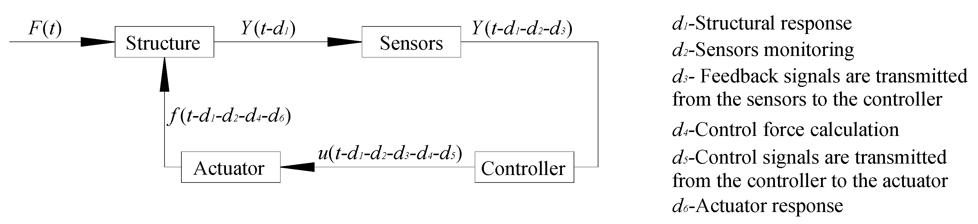
2.1. Time-Delay Sources

As shown in Figure 1 about the workflow of a control system, the time-delay resulted from different types of time-delays. A new reduced-order controller for buildings is conducted to compensate for the time-delay d₄ [23]. Moreover, the compensation method for the time-delay d₆ configurated the important research content [22]. The others (d₁, d₂, d₃ and d₅) are described in this section.

For a building, owing to the limited in-plane stiffness of a floor, the stress wave generated by a horizontal external excitation propagates in each floor. The propagation time is the structural response delay d₁. The state-space equation is described as,

$$\{\begin{array}{l}{\dot{Z}}_{str}\left(t\right)=A_{str}{Z}_{str}\left(t\right)+B_{str}w\left(t\right)\\ Y_{str}\left(t\right)=C_{str}{Z}_{str}\left(t-d_1\right)+D_{str}w\left(t-d_1\right)\end{array}$$

(1)

where A_str is the state matrix, B_str is the excitation matrix, C_str is the state output matrix and D_str is the direct transmission matrix of a building. Z_str is the state vector and Y_str is the output vector. w is an external excitation.

The structural response delay of each floor of a high-rise building is not equal, so the input equation of its control system cannot be simply described as the second equation of Equation (1) which in this article only describes this related parameter. In addition, the first equation of Equation (1) representing the dynamic equilibrium of the structure cannot consider the addition of the time delay d₁, since it is contained directly in the equilibrium equation. In result, the structural response delay is not considered in this paper.

Taking a force balanced accelerometer as an example, the process of monitoring structural responses takes time which is called the monitoring time-delay of sensors d₂. The state-space equation of a monitoring system is,

$$\{\begin{array}{l}{\dot{Z}}_{sen}\left(t\right)=A_{sen}{Z}_{sen}\left(t\right)+B_{sen}{a}_{str}\left(t\right)\\ U_{sen}\left(t\right)=C_{sen}{Z}_{sen}\left(t-d_2\right)+D_{sen}{a}_{str}\left(t-d_2\right)\end{array}$$

(2)

where A_sen is the state matrix, B_sen is the excitation matrix, C_sen is the state output matrix and D_sen is the direct transmission matrix of a monitoring system. Z_sen is the state vector and U_sen indicates the output vector of sensors. a_str is structural acceleration responses.

The distribution of sensors in a building is scattered. There is a certain distance between the sensors and its control room. The required time from the output signals of sensors to their acquisition device is called the time-delay d₃. The transmitted time from the control signals to the actuator is called the time-delay d₅. According to the reference [30], since the speed of electromagnetic waves in a line is fast enough, which is about 2.45 m/s, the time delays (d₃ and d₅) can be ignored.

The measurement of acceleration signals is easier to be conducted than the displacement and velocity signals [31]. The acquisition device converts the received feedback voltage signals into the acceleration signals, and the measurement of acceleration signals is,

$$a_{sen}\left(t\right)=U_{sen}\left(t\right)/K_a$$

(3)

where K_a is the sensor sensitivity coefficient.

In view of the acceleration feedback signals, a new state observer in the reference [31] is adopted to estimate the whole state vectors of an observer-based control system. The control force calculation time-delay d₄ consists of two parts (d₄₁ + d₄₂). The time required for the estimation process is called the time-delay d₄₁. The state-space equation of the observer-based control system is,

$$\{\begin{array}{l}{\dot{Z}}_{obs}\left(t\right)=A_{obs}{Z}_{obs}\left(t\right)+B_{obs}{a}_{sen}\left(t\right)\\ Y_{obs}\left(t\right)=C_{obs}{Z}_{obs}\left(t-d_{41}\right)+D_{obs}{a}_{sen}\left(t-d_{41}\right)\end{array}$$

(4)

where A_obs is the state matrix, B_obs is the excitation matrix, C_obs is the state output matrix and D_obs is the direct transmission matrix of an observer-based controller. Z_obs is the state vector and Y_obs is the output vector.

Based on the estimated states, the output control forces can be calculated according to a specific algorithm,

$$f\left(t\right)=-G{Y}_{obs}\left(t\right)$$

(5)

where G represents a feedback gain matrix.

The time required for calculating control forces is called the time-delay d₄₂. The state-space equation of a control system is thereby written as,

$$\{\begin{array}{l}{\dot{Z}}_{con}\left(t\right)=A_{con}{Z}_{con}\left(t\right)+B_{con}{Y}_{obs}\left(t\right)\\ f\left(t\right)=C_{con}{Z}_{con}\left(t-d_{42}\right)+D_{con}{Y}_{obs}\left(t-d_{42}\right)\end{array}$$

(6)

where A_con is the state matrix, B_con is the control matrix, C_con is the state output matrix and D_con is the direct transmission matrix. Z_con is the state vector.

The control forces provided by a DC motor are discussed in the reference [24] as,

$$u\left(t\right)=-\frac{L_a}{R_a}\dot{u}\left(t\right)-\frac{K_b{K}_i{K}_g^2}{R_a{r}_m^2}\left[{\dot{x}}_a\left(t\right)-{\dot{x}}_n\left(t\right)\right]+\frac{K_i{K}_g}{R_a{r}_m}v\left(t\right)$$

(7)

where v is the applied voltage, L_a indicates the armature inductance, R_a indicates the armature resistance, K_b represents the back electromotive force constant, K_i is the motor torque constant, K_g and r_m are the gear ratio and the lead of the ball screw, respectively. ${\dot{x}}_a$ and ${\dot{x}}_n$ are the relative velocities of the auxiliary mass and its installed floor, respectively.

The control-force equation and its transform are acquired from Equation (7) as,

$$\{\begin{array}{l}\dot{u}\left(t\right)=\left(-\frac{R_a}{L_a}\right)u\left(t\right)+\left[\begin{array}{ccc}\frac{K_i{K}_g}{L_a{r}_m}& -\frac{K_b{K}_i{K}_g^2}{L_a{r}_m^2}& \frac{K_b{K}_i{K}_g^2}{L_a{r}_m^2}\end{array}\right]\left\{\begin{array}{c}v\left(t\right)\\ {\dot{x}}_a\\ {\dot{x}}_n\end{array}\right\}\\ Y\left(t\right)=u\left(t-d_6\right)\end{array}$$

(8)

In conclusion, the time delays (d₁, d₃ and d₅) can be ignored in the paper, and the total time-delay of the control system is,

$$\tau =d_2+d_4+d_6$$

(9)

2.2. Impact Analysis of Multi-Time Delays

The force equilibrium equation is,

$$M\ddot{X}\left(t\right)+C\dot{X}\left(t\right)+KX\left(t\right)=B_{w}w\left(t\right)+{\displaystyle \sum _{i=1}^m{B}_{si}{u}_i\left(t\right)},$$

(10)

where M, C and K indicate the mass, damping and stiffness matrix. u_i is the force of the ith controller. B_s indicates the location matrices of control forces, and B_w indicates the location matrices of external excitations. X is the displacement of the system.

The ith time-delay is ${\tau }_i$, and Equation (1) is expressed as,

$$\dot{Z}(t)=AZ\left(t\right)+{\displaystyle \sum _{i=1}^m{B}_i{u}_i\left(t-{\tau }_i\right)}+Ew\left(t\right)$$

(11)

where Z indicates the state vector, which includes structural displacement and velocity responses. A is the state matrix, B_i is the control matrix of the ith force and E is the excitation matrix,

$$A=\left[\begin{array}{cc}0& I\\ -M^{-1}K& -M^{-1}C\end{array}\right],B_i=\left[\begin{array}{c}0\\ M^{-1}{B}_{si}\end{array}\right],E=\left[\begin{array}{c}0\\ M^{-1}{B}_w\end{array}\right].$$

(12)

To clarify the difference between the system with a single-controller (System1) and the system with multi-controllers (System2 which includes two controllers: AMD1 and AMD2), a four-story frame along its minor-axis is used as an example to compare and analyze these above methods, which is shown in Figure 2. The above frame is constructed by steel with a damping ratio of 0.02. The important parameters are revealed in

Table 1. The important parameters of different AMD systems.

Index	System1	System2
The weight of the auxiliary mass (kg)	20 × 1	10 × 2
The effective stroke (m)	$\pm$0.4	$\pm$0.4
The maximum driving force (N)	±1000 × 1	±500 × 2

. More details and the dynamic properties of the structure are found in the reference [32].

Three cases are considered in this paper: the control systems without time delays, the systems with equal time delays and the systems with unequal time delays. Under the SN direction of the El-Centro seismic wave, the equal time delays are assumed to be 0.05 s (${\tau }_1={\tau }_2=0.05 \mathrm{s}$), and the time-delay difference is set as 0.02 s, which means that ${\tau }_1=0.04 \mathrm{s}$ and ${\tau }_2=0.04+0.02=0.06 \mathrm{s}$.

Table 2. The acceleration control effects (%).

Index	No Time Delays		With Equal Time Delays		With Unequal Time Delays
	System1	System2	System1	System2	System1	System2
2nd floor	36.21	36.08	−11.19	−17.29	—	−15.97
3rd floor	38.51	38.37	−8.70	−13.88	—	−12.94
4th floor	39.95	39.79	−7.27	−11.56	—	−9.15

shows the acceleration control effects, and the control parameters are shown in Figure 3, Figure 4, Figure 5, Figure 6, Figure 7 and Figure 8. The ratio between the reduction of structural responses and the responses without control is defines as Control effect. The control forces and strokes constitute AMD parameters.

From Table 2, the multi-controllers can basically ensure synchronization in the systems without time delays. Therefore, the control effects of System2 are close to those of System1. When the equal time delays are considered, the acceleration control effects to the 8th floor of System1 and System2 decrease by 47.41% and 52.05%, respectively. This is due to the fact that the structural equivalent damping becomes smaller as the time delays increase. The energy dissipation capacity of the control system is obviously reduced. This leads to an increase in the acceleration responses and a significant decrease in the control effects. The decrease of control effect of System2 is larger than that of System1 with the same time delays, that is, the time-delay robustness of System2 is less than that of System1. When the unequal time delays are considered, the acceleration control effect to the 8th floor of System2 decrease by 53.37%. Compared with the case of the equal time delays, the control effects of System2 are slightly decreased.

As shown in Figure 3 and Figure 4, the maximum strokes of System2 are close to those of System1 when without time-delay effect. However, compared with the whole forces of System1, the sum of the forces of the sub-controllers is larger, which means relatively speaking, the output of System1 is lower than that of System2. In System2, the differences of the control parameters are relatively close to zero, indicating that the multi-controllers operate synchronously.

As shown Figure 3, Figure 4, Figure 5 and Figure 6, equal time-delays reduce the acceleration control effects of System1 and System2. Comparing Figure 3, Figure 4 and Figure 5, the control forces of System1 and System2 significantly increase, but their strokes are basically unchanged. This is caused by the less impact of time-delays on the displacement feedback gain of the auxiliary mass. Comparing Figure 4 with Figure 6, the differences of the control parameters of the multi-controllers with equal time delays are nearly equivalent to those of the systems without time delays, which means that equal time-delays have little influence on the synchronization of System2.

As shown in Figure 7 and Figure 8, the differences of the control forces are obvious when there are unequal time delays in System2, which means that unequal time-delays have an impact on the synchronization of System2, where System2 consists of two relatively independent subsystems. However, compared to the differences of the control forces, the differences of the strokes are relatively smaller. This is due to the fact that time-delays have less influence on the feedback gains to the displacements of the auxiliary mass.

To analyze the impact of the time-delay differences on different systems, the time delay difference is increased from 0 to 0.02 s, and the corresponding maximum strokes and maximum control forces of System2 are plotted in Figure 9. As the time-delay differences increase, for the AMD-1, the amplitude of the control forces become larger while the amplitude of the strokes remains stable, which is consistent with the previous results.

3. A Compensation Strategy Using an H_∞ Control Law

3.1. Design Principle

The state-space equation of the multi-time-delay system is,

$$\{\begin{array}{l}\dot{Z}\left(t\right)=AZ\left(t\right)+{\displaystyle \sum _{i=1}^m{B}_i{u}_i\left(t-{\tau }_i\right)}+Ew\left(t\right)\\ Y\left(t\right)=CZ\left(t\right)+{\displaystyle \sum _{i=1}^m{D}_i{u}_i\left(t-{\tau }_i\right)}+Fw\left(t\right)\end{array}$$

(13)

where ${\tau }_i$ denotes the time-delay of ith controller, u_i represents the ith control force. Y is the controlled vectors, which includes the dynamic responses and the control forces. C indicates the state output matrix, D_i indicates the direct transmission matrix of the control forces, and F indicates the direct transmission matrix of the external excitations. The expressions are as following,

$$C=\left[\begin{array}{cc}I& 0\\ 0& I\\ -M^{-1}K& -M^{-1}C\\ 0& 0\end{array}\right],D_i=\left[\begin{array}{c}0\\ 0\\ M^{-1}{B}_{si}\\ 1\end{array}\right],F=\left[\begin{array}{c}0\\ 0\\ M^{-1}{B}_w\\ 0\end{array}\right].$$

(14)

For the system (13), the negative feedback control forces are,

$$u_i\left(t-{\tau }_i\right)=-G_{ci}Z\left(t-{\tau }_i\right)$$

(15)

where G_ci denotes the ith feedback gain.

The system is,

$$\{\begin{array}{l}\dot{Z}\left(t\right)=AZ\left(t\right)+{\displaystyle \sum _{i=1}^m\left(-B_i{G}_{ci}\right)Z\left(t-{\tau }_i\right)}+Ew\left(t\right)\\ Y\left(t\right)=CZ\left(t\right)+{\displaystyle \sum _{i=1}^m\left(-D_i{G}_{ci}\right)Z\left(t-{\tau }_i\right)}+Fw\left(t\right)\end{array}$$

(16)

According to the reference [33], this paper introduces the following definitions and lemmas to facilitate the analysis. Regarding the system (16), only when there are symmetric positive-definite matrices P and S_i (i = 1, 2, …, m), Lyapunov function is described as,

$$V\left(Z\right)=Z^{T}PZ+{\displaystyle \sum _{i=1}^m{\displaystyle {\int }_{\hspace{0.17em}t-{\tau }_i}^t{Z}^T}\left(\sigma \right)S_{i}Z\left(\sigma \right)d\sigma }$$

(17)

where V(Z) denotes a positive-definite matrix.

When the system (16) is asymptotically stable, its derivative $\dot{V}\left(Z\right)$ is a negative-definite function. Then,

$$\begin{array}{cc}\hfill \dot{V}\left(Z\right)& ={\dot{Z}}^T\left(t\right)PZ\left(t\right)+Z^T\left(t\right)P\dot{Z}\left(t\right)+{\displaystyle \sum _{i=1}^m\left[Z^T\left(t\right)S_{i}Z\left(t\right)-Z^T\left(t-{\tau }_i\right)S_{i}Z\left(t-{\tau }_i\right)\right]}\hfill \\ & ={\left[AZ\left(t\right)+{\displaystyle \sum _{i=1}^m\left(-B_i{G}_{ci}\right)Z\left(t-{\tau }_i\right)+Ew\left(t\right)}\right]}^{T}PZ\left(t\right)\hfill \\ & +Z^T\left(t\right)P\left[AZ\left(t\right)+{\displaystyle \sum _{i=1}^m\left(-B_i{G}_{ci}\right)Z\left(t-{\tau }_i\right)+Ew\left(t\right)}\right]+{\displaystyle \sum _{i=1}^m\left[Z^T\left(t\right)S_{i}Z\left(t\right)-Z^T\left(t-{\tau }_i\right)S_{i}Z\left(t-{\tau }_i\right)\right]}\hfill \end{array}$$

(18)

Then,

$$\begin{array}{cc}\hfill \dot{V}\left(Z\right)& =Z^T\left(t\right)\left[PA+{\left(PA\right)}^T+{\displaystyle \sum _{i=1}^m{S}_i}\right]Z\left(t\right)-{\displaystyle \sum _{i=1}^m\left[Z^T\left(t-{\tau }_i\right)S_{i}Z\left(t-{\tau }_i\right)\right]}\hfill \\ & -{\displaystyle \sum _{i=1}^m\left\{\left[Z^T\left(t\right)P\left(B_i{G}_{ci}\right)Z\left(t-{\tau }_i\right)\right]-{\left[Z^T\left(t\right)P\left(B_i{G}_{ci}\right)Z\left(t-{\tau }_i\right)\right]}^T\right\}}\hfill \\ & +w^T\left(t\right)\left(E^{T}P\right)Z\left(t\right)+Z^T\left(t\right)\left(PE\right)w\left(t\right)\hfill \end{array}$$

(19)

Equation (19) is written as the block matrixes,

$$\dot{V}\left[Z\left(t\right)\right]={\left\{\begin{array}{c}Z\left(t\right)\\ Z\left(t-{\tau }_1\right)\\ Z\left(t-{\tau }_2\right)\\ ⋮\\ Z\left(t-{\tau }_m\right)\\ w\left(t\right)\end{array}\right\}}^T\mathsf{\Xi }\left\{\begin{array}{c}Z\left(t\right)\\ Z\left(t-{\tau }_1\right)\\ Z\left(t-{\tau }_2\right)\\ ⋮\\ Z\left(t-{\tau }_m\right)\\ w\left(t\right)\end{array}\right\}$$

(20)

where $\mathsf{\Xi }$ is the coefficient matrix which can be expressed as,

$$\mathsf{\Xi }=\left[\begin{array}{cccccc}PA+{\left(PA\right)}^T+{\displaystyle \sum _{i=1}^m{S}_i}& -P\left(B_1{G}_{c1}\right)& -P\left(B_2{G}_{c2}\right)& \cdots & -P\left(B_m{G}_{cm}\right)& PE\\ -{\left(B_1{G}_{c1}\right)}^{T}P& -{\displaystyle \sum _{i=1}^m{S}_i}& 0& \cdots & 0& 0\\ -{\left(B_2{G}_{c2}\right)}^{T}P& 0& -{\displaystyle \sum _{i=1}^m{S}_i}& \cdots & 0& 0\\ ⋮& ⋮& ⋮& \ddots & ⋮& ⋮\\ -{\left(B_m{G}_{cm}\right)}^{T}P& 0& 0& \cdots & -{\displaystyle \sum _{i=1}^m{S}_i}& 0\\ E^{T}P& 0& 0& \cdots & 0& 0\end{array}\right]$$

(21)

The performance index of the system (16) is given as,

$$J_z={\displaystyle {\int }_{\hspace{0.17em}\sigma =0}^{\hspace{0.17em}t}\left[Y^T\left(\sigma \right)Y\left(\sigma \right)-{\gamma }^2{w}^T\left(\sigma \right)w\left(\sigma \right)\right]}d\sigma$$

(22)

where $\gamma$ is a given positive scalar.

Then,

$$J_z={\displaystyle {\int }_{\hspace{0.17em}\sigma =0}^{\hspace{0.17em}t}\left\{Y^T\left(\sigma \right)Y\left(\sigma \right)-{\gamma }^2{w}^T\left(\sigma \right)w\left(\sigma \right)+\dot{V}\left[Z\left(\sigma \right)\right]\right\}}d\sigma -V\left[Z\left(t\right)\right]$$

(23)

Owing to $V\left[Z\left(t\right)\right]>0$, then,

$$J_z\le {\displaystyle {\int }_{\hspace{0.17em}\sigma =0}^{\hspace{0.17em}t}\left\{Y^T\left(\sigma \right)Y\left(\sigma \right)-{\gamma }^2{w}^T\left(\sigma \right)w\left(\sigma \right)+\dot{V}\left[Z\left(\sigma \right)\right]\right\}}d\sigma$$

(24)

According to the system (16), then,

$$\begin{array}{l}{Y}^T\left(\sigma \right)Y\left(\sigma \right)-{\gamma }^2{w}^T\left(\sigma \right)w\left(\sigma \right)={\left[CZ\left(\sigma \right)+{\displaystyle \sum _{i=1}^m\left(-D_i{G}_{ci}\right)Z\left(\sigma -{\tau }_i\right)}+Fw\left(\sigma \right)\right]}^T\\ \cdot \left[CZ\left(\sigma \right)+{\displaystyle \sum _{i=1}^m\left(-D_i{G}_{ci}\right)Z\left(\sigma -{\tau }_i\right)}+Fw\left(\sigma \right)\right]-{\gamma }^2{w}^T\left(\sigma \right)w\left(\sigma \right)\end{array}$$

(25)

Equation (25) is written as the block matrixes, then,

$$Y^T\left(\sigma \right)Y\left(\sigma \right)-{\gamma }^2{w}^T\left(\sigma \right)w\left(\sigma \right)={\left\{\begin{array}{c}Z\left(\sigma \right)\\ Z\left(\sigma -{\tau }_1\right)\\ Z\left(\sigma -{\tau }_2\right)\\ ⋮\\ Z\left(\sigma -{\tau }_m\right)\\ w\left(\sigma \right)\end{array}\right\}}^T\mathsf{\Psi }\left\{\begin{array}{c}Z\left(\sigma \right)\\ Z\left(\sigma -{\tau }_1\right)\\ Z\left(\sigma -{\tau }_2\right)\\ ⋮\\ Z\left(\sigma -{\tau }_m\right)\\ w\left(\sigma \right)\end{array}\right\}$$

(26)

where $\mathsf{\Psi }$ is the coefficient matrix which can be expressed as,

$$\mathsf{\Psi }=\left[\begin{array}{cccccc}{C}^{T}C& -C^T\left(D_1{G}_{c1}\right)& -C^T\left(D_2{G}_{c2}\right)& \cdots & -C^T\left(D_m{G}_{cm}\right)& C^{T}F\\ -{\left(D_1{G}_{c1}\right)}^{T}C& {\left(D_1{G}_{c1}\right)}^T\left(D_1{G}_{c1}\right)& {\left(D_1{G}_{c1}\right)}^T\left(D_2{G}_{c2}\right)& \cdots & {\left(D_1{G}_{c1}\right)}^T\left(D_m{G}_{cm}\right)& -{\left(D_1{G}_{c1}\right)}^{T}F\\ -{\left(D_2{G}_{c2}\right)}^{T}C& {\left(D_2{G}_{c2}\right)}^T\left(D_1{G}_{c1}\right)& {\left(D_2{G}_{c2}\right)}^T\left(D_2{G}_{c2}\right)& \cdots & {\left(D_2{G}_{c2}\right)}^T\left(D_m{G}_{cm}\right)& -{\left(D_2{G}_{c2}\right)}^{T}F\\ ⋮& ⋮& ⋮& \ddots & ⋮& ⋮\\ -{\left(D_m{G}_{cm}\right)}^{T}C& {\left(D_m{G}_{cm}\right)}^T\left(D_1{G}_{c1}\right)& {\left(D_m{G}_{cm}\right)}^T\left(D_2{G}_{c2}\right)& \cdots & {\left(D_m{G}_{cm}\right)}^T\left(D_m{G}_{cm}\right)& -{\left(D_m{G}_{cm}\right)}^{T}F\\ F^{T}C& -F^T\left(D_1{G}_{c1}\right)& -F^T\left(D_2{G}_{c2}\right)& \cdots & -F^T\left(D_m{G}_{cm}\right)& F^{T}F-{\gamma }^{2}I\end{array}\right]$$

(27)

Then,

$$J_z\le {\displaystyle {\int }_{\hspace{0.17em}\sigma =0}^{\hspace{0.17em}t}\left({\left\{\begin{array}{c}Z\left(\sigma \right)\\ Z\left(\sigma -{\tau }_1\right)\\ Z\left(\sigma -{\tau }_2\right)\\ ⋮\\ Z\left(\sigma -{\tau }_m\right)\\ w\left(\sigma \right)\end{array}\right\}}^T\mathsf{\Omega }\left\{\begin{array}{c}Z\left(\sigma \right)\\ Z\left(\sigma -{\tau }_1\right)\\ Z\left(\sigma -{\tau }_2\right)\\ ⋮\\ Z\left(\sigma -{\tau }_m\right)\\ w\left(\sigma \right)\end{array}\right\}\right)d\sigma }$$

(28)

where $\mathsf{\Omega }$ is the coefficient matrix which can be expressed as,

$$\begin{array}{l}\mathsf{\Omega }=[\begin{array}{cc}PA+{\left(PA\right)}^T+{\displaystyle \sum _{i=1}^m{S}_i}+C^{T}C& -P\left(B_1{G}_{c1}\right)-C^T\left(D_1{G}_{c1}\right)\\ -{\left(B_1{G}_{c1}\right)}^{T}P-{\left(D_1{G}_{c1}\right)}^{T}C& {\left(D_1{G}_{c1}\right)}^T\left(D_1{G}_{c1}\right)-{\displaystyle \sum _{i=1}^m{S}_i}\\ -{\left(B_2{G}_{c2}\right)}^{T}P-{\left(D_2{G}_{c2}\right)}^{T}C& {\left(D_2{G}_{c2}\right)}^T\left(D_1{G}_{c1}\right)\\ ⋮& ⋮\\ -{\left(B_m{G}_{cm}\right)}^{T}P-{\left(D_m{G}_{cm}\right)}^{T}C& {\left(D_m{G}_{cm}\right)}^T\left(D_1{G}_{c1}\right)\\ E^{T}P+F^{T}C& F^T\left(D_1{G}_{c1}\right)\end{array}\\ \begin{array}{cccc}-P\left(B_2{G}_{c2}\right)-C^T\left(D_2{G}_{c2}\right)& \cdots & -P\left(B_m{G}_{cm}\right)-C^T\left(D_m{G}_{cm}\right)& PE+C^{T}F\\ {\left(D_1{G}_{c1}\right)}^T\left(D_2{G}_{c2}\right)& \cdots & {\left(D_1{G}_{c1}\right)}^T\left(D_m{G}_{cm}\right)& {\left(D_1{G}_{c1}\right)}^{T}F\\ {\left(D_2{G}_{c2}\right)}^T\left(D_2{G}_{c2}\right)-{\displaystyle \sum _{i=1}^m{S}_i}& \cdots & {\left(D_2{G}_{c2}\right)}^T\left(D_m{G}_{cm}\right)& {\left(D_2{G}_{c2}\right)}^{T}F\\ ⋮& \ddots & ⋮& ⋮\\ {\left(D_m{G}_{cm}\right)}^T\left(D_2{G}_{c2}\right)& \cdots & {\left(D_m{G}_{cm}\right)}^T\left(D_m{G}_{cm}\right)-{\displaystyle \sum _{i=1}^m{S}_i}& {\left(D_m{G}_{cm}\right)}^{T}F\\ F^T\left(D_2{G}_{c2}\right)& \cdots & F^T\left(D_m{G}_{cm}\right)& F^{T}F-{\gamma }^{2}I\end{array}]\end{array}$$

(29)

The closed loop system shown by Equation (13) can be stabilized by a state-feedback compensation controller with an H_∞ performance index according to the references [34,35]. Only when there are symmetric positive-definite matrices P and S_i (i = 1, 2, …, m), the inequality $\mathsf{\Omega }<0$ is satisfied. Then,

$$J_z\le {\displaystyle {\int }_{\hspace{0.17em}\sigma =0}^{\hspace{0.17em}t}\left({\left\{\begin{array}{c}Z\left(\sigma \right)\\ Z\left(\sigma -{\tau }_1\right)\\ Z\left(\sigma -{\tau }_2\right)\\ ⋮\\ Z\left(\sigma -{\tau }_m\right)\\ w\left(\sigma \right)\end{array}\right\}}^T\mathsf{\Omega }\left\{\begin{array}{c}Z\left(\sigma \right)\\ Z\left(\sigma -{\tau }_1\right)\\ Z\left(\sigma -{\tau }_2\right)\\ ⋮\\ Z\left(\sigma -{\tau }_m\right)\\ w\left(\sigma \right)\end{array}\right\}\right)d\sigma }<0$$

(30)

Then,

$${\displaystyle {\int }_{\hspace{0.17em}\sigma =0}^{\infty }\left[Y^T\left(\sigma \right)Y\left(\sigma \right)\right]}d\sigma <{\gamma }^2{\displaystyle {\int }_{\hspace{0.17em}\sigma =0}^{\infty }\left[w^T\left(\sigma \right)w\left(\sigma \right)\right]}d\sigma$$

(31)

Or,

$${\Vert Y\left(\sigma \right)\Vert }^2<{\gamma }^2{\Vert w\left(\sigma \right)\Vert }^2$$

(32)

According to Schur’s complement in the reference [36], the inequality $\mathsf{\Omega }<0$ is,

$$\left[\begin{array}{ccccccc}PA+{\left(PA\right)}^T+{\displaystyle \sum _{i=1}^m{S}_i}& -P\left(B_1{G}_{c1}\right)& -P\left(B_2{G}_{c2}\right)& \cdots & -P\left(B_m{G}_{cm}\right)& PE& C^T\\ -{\left(B_1{G}_{c1}\right)}^{T}P& -{\displaystyle \sum _{i=1}^m{S}_i}& 0& \cdots & 0& 0& -{\left(D_1{G}_{c1}\right)}^T\\ -{\left(B_2{G}_{c2}\right)}^{T}P& 0& -{\displaystyle \sum _{i=1}^m{S}_i}& \cdots & 0& 0& -{\left(D_2{G}_{c2}\right)}^T\\ ⋮& ⋮& ⋮& \ddots & ⋮& ⋮& ⋮\\ -{\left(B_m{G}_{cm}\right)}^{T}P& 0& 0& \cdots & -{\displaystyle \sum _{i=1}^m{S}_i}& 0& -{\left(D_m{G}_{cm}\right)}^T\\ E^{T}P& 0& 0& \cdots & 0& -{\gamma }^{2}I& F^T\\ C& -\left(D_1{G}_{c1}\right)& -\left(D_2{G}_{c2}\right)& \cdots & -\left(D_m{G}_{cm}\right)& F& -I\end{array}\right]<0$$

(33)

The variable substitution method [37] is referred for transforming the inequality (33) from a nonlinear matrix inequality into a linear matrix inequality. Supposing X_i = P(B_iG_ci) and Y_i = D_iG_ci. Only when there are symmetric positive-definite matrices P, S_i and matrices X_i, Y_i (i = 1, 2, …, m), the following inequality is satisfied.

$$\left[\begin{array}{ccccccc}PA+{\left(PA\right)}^T+{\displaystyle \sum _{i=1}^m{S}_i}& -X_1& -X_2& \cdots & -X_m& PE& C^T\\ -X_1^T& -{\displaystyle \sum _{i=1}^m{S}_i}& 0& \cdots & 0& 0& -Y_1^T\\ -X_2^T& 0& -{\displaystyle \sum _{i=1}^m{S}_i}& \cdots & 0& 0& -Y_2^T\\ ⋮& ⋮& ⋮& \ddots & ⋮& ⋮& ⋮\\ -X_m^T& 0& 0& \cdots & -{\displaystyle \sum _{i=1}^m{S}_i}& 0& -Y_m^T\\ E^{T}P& 0& 0& \cdots & 0& -{\gamma }^{2}I& F^T\\ C& -Y_1& -Y_2& \cdots & -Y_m& F& -I\end{array}\right]<0$$

(34)

The ith control force is,

$$u_i\left(t\right)=\left[{\left(P{B}_i\right)}^{-1}{X}_i\right]Z\left(t\right)$$

(35)

Then the ith feedback gain matrix is,

$$G_{ci}=-{\left(P{B}_i\right)}^{-1}{X}_i$$

(36)

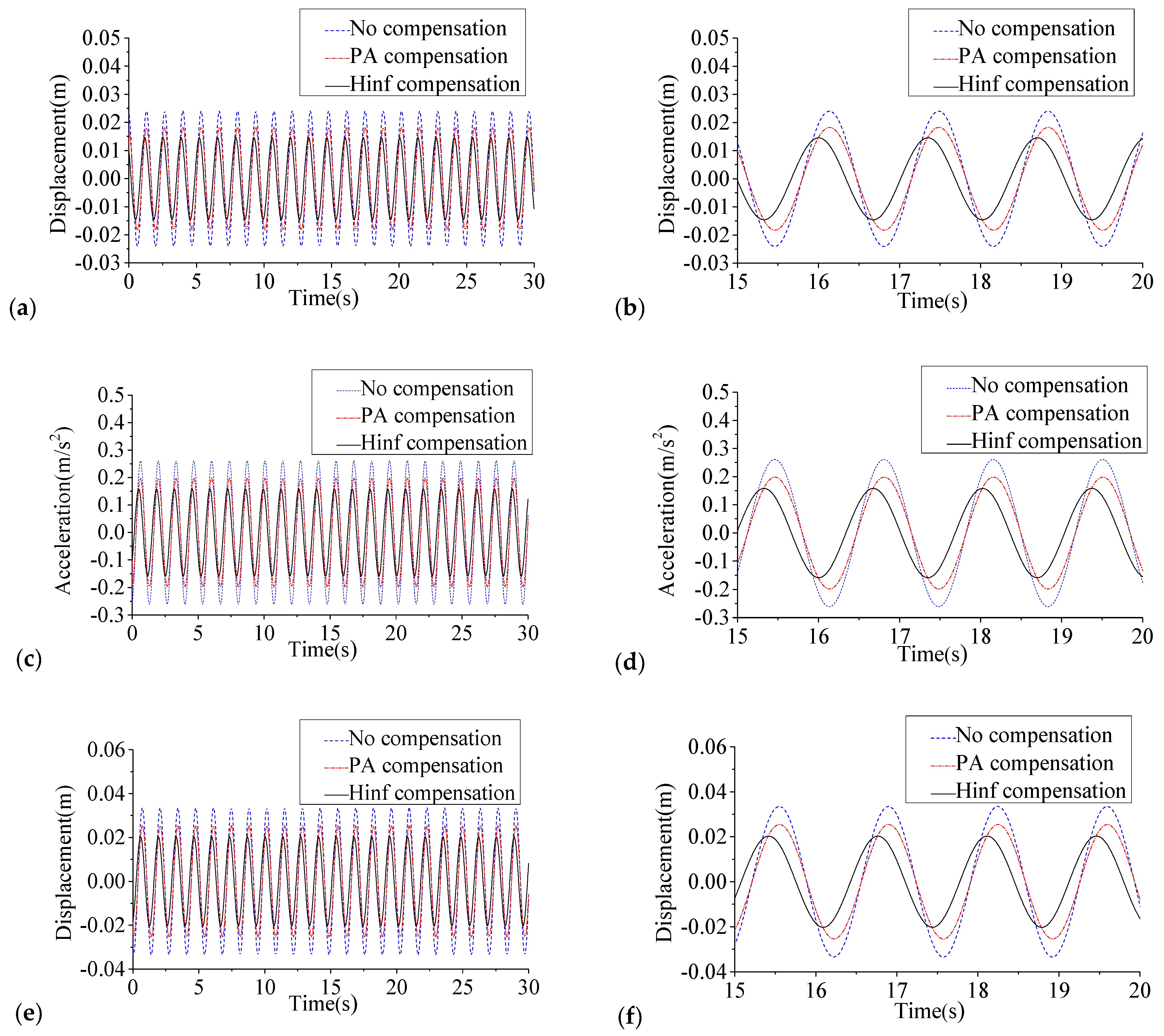
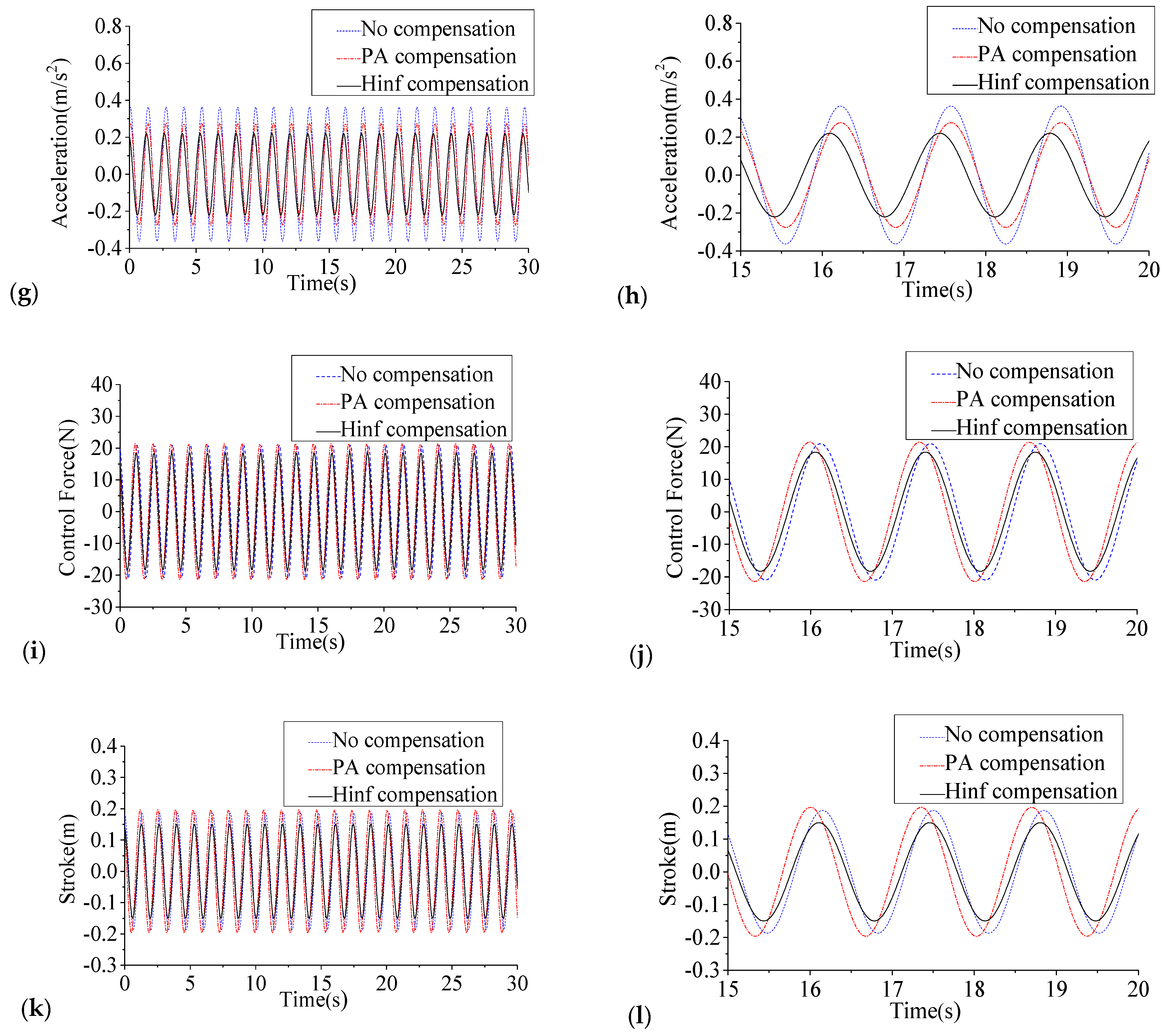
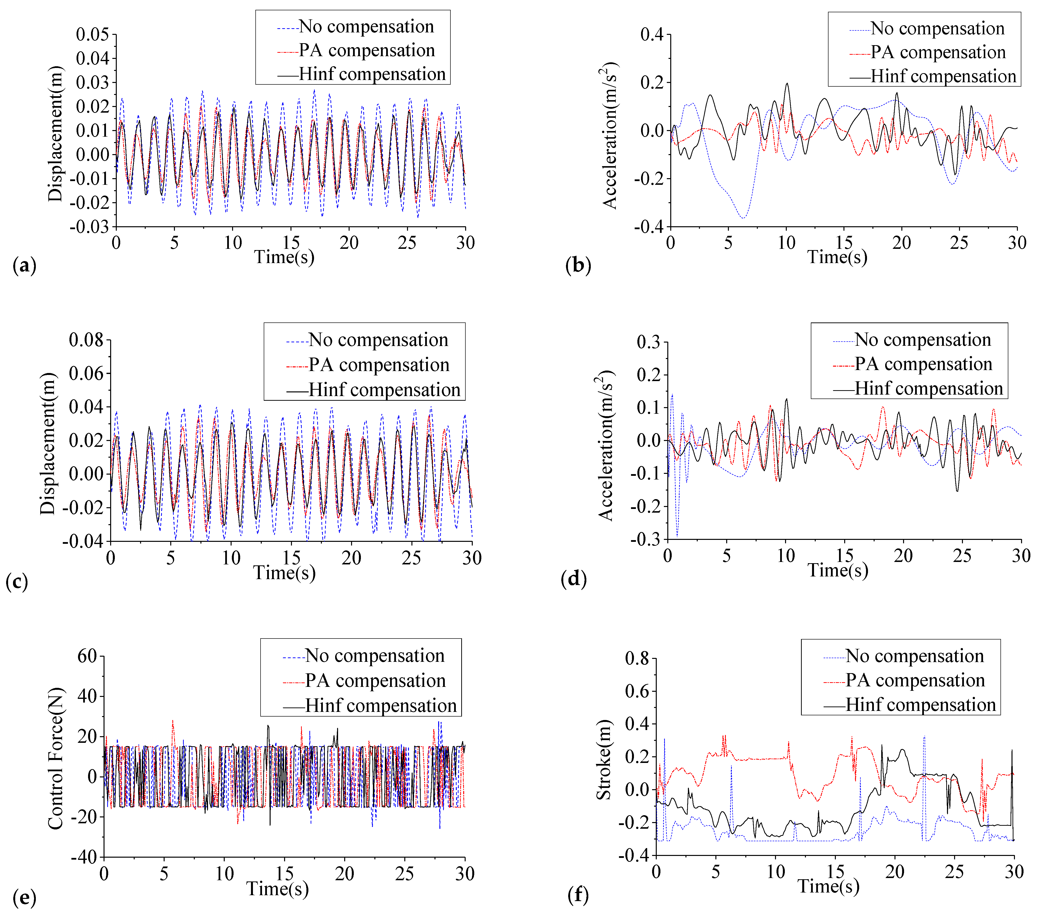
3.2. Numerical and Experimental Verification

Three systems are built for the four-story frame (Figure 2): a time-delay system without compensation, the system with pole-assignment (PA) compensation [18] and the system with H_∞ compensation. The latter two systems include multiple time delays. In PA compensation method, by appropriately changing the compensation gains, the poles of the time-delay system are located in a target area. Conservatively, the multiple time delays are defined as 0.4 s (${\tau }_1$) and 0.6 s (${\tau }_2$) since one of the time delays in the experimental system is about 0.2~0.3 s after testing. In the experimental system, a control-force signal is provided to the servo motor, and the actual system time delay is the time required to apply the control forces to the structure. For engineering applications, it is difficult to measure the displacement and velocity responses of a building. In the study, a state observer using structural accelerations is built from the reference [31]. Finally, the simulink diagram of the experimental system is shown in Figure 10.

Under an excitation load, the numerical and measured results are listed in

Table 3. The control effects under the numerical results (mean square values).

Index		No Control	No Compensation		PA Compensation		H∞ Compensation
			Responses	Effect (%)	Responses	Effect (%)	Responses	Effect (%)
Displacement (cm)	2nd floor	1.54	1.70	−10.22	1.29	16.24	1.03	33.26
	4th floor	2.15	2.37	−10.25	1.80	16.21	1.43	33.23
Acceleration (cm/s2)	2nd floor	16.76	18.48	−10.23	14.04	16.23	11.19	33.25
	4th floor	23.33	25.72	−10.25	19.54	16.23	15.58	33.24
Control force (N)		—	14.80	—	15.13	—	12.96	—
Stroke (cm)		—	13.23	—	13.91	—	10.60	—

and

Table 4. The control effects under the measured results (mean square values).

Index		No Control	No Compensation		PA Compensation		H∞ Compensation
			Responses	Effect (%)	Responses	Effect (%)	Responses	Effect (%)
Displacement (cm)	2nd floor	1.58	1.62	−2.53	1.11	29.75	1.01	36.08
	4th floor	2.67	2.62	1.87	1.86	30.34	1.69	36.70
Acceleration (cm/s2)	2nd floor	14.95	16.81	−12.44	5.86	60.80	6.09	59.26
	4th floor	11.74	16.03	−36.54	4.29	63.46	3.84	67.29
Control force (N)		—	14.90	—	14.19	—	14.12	—
Stroke (cm)		—	17.55	—	15.13	—	11.82	—

. The control effects and the relevant control parameters are shown in Figure 11 and Figure 12.

From Figure 11 and Figure 12 and Table 3 and Table 4, the maximum structural responses calculated by the numerical method are basically consistent with the measured results, which are closely related to the accuracy of the sensor and numerical model. The structural responses of the numerical results follow the sine law under a sinusoidal excitation load. On the contrary, the structural responses of the measured results do not fully follow the sine law due to the interaction effect between the controller and the frame, and the coupling effect of the structural horizontal and vertical vibrations. The strokes of the numerical results illustrated in Figure 11f are obviously different from those of the measured results illustrated in Figure 12f. There are three adverse aspects: the environmental interference signals, the inhomogeneous magnetic field between the rotor and stator and the unsmooth support track of the motor. In addition, due to the mechanical construction of the servo motor, the frequency of the control forces in the measured test is inconsistent with the numerical simulation. As a result, there are significant differences between the control forces of the numerical results and those of the measured results, which are shown in Figure 11e and Figure 12e, respectively.

The control system without compensation has a negative impact on reduction of the structural responses. By contrast, the control systems with the multiple time delays tend to reduce the dynamic responses, and the efficiency of PA compensation system is slightly worse than that of H_∞ compensation system, especially the acceleration control effects. The reason is that the calculation process of the former system excludes the optimal control-gain selection process. Hence, the selected PA compensation gains are only a fixed value. Since the selected control gains of H_∞ compensation are a global optimal solution, its strokes are relatively smaller than those of PA compensation. Otherwise, the control forces of PA compensation are much higher than those of H_∞ compensation. The imaginary part of the PA compensation gains should be zero so that its state vectors and control forces are real constants. However, this will not happen in H_∞ compensation system. Its auxiliary mass runs smoothly and the control forces are stable, indicating that the H_∞ compensation system has a better performance.

4. Conclusions

Impact analysis of multi-time-delays on the performance of an AMD system is completely conducted. For the negative effect of multi-time-delay in each subsystem, a new compensation controller is designed using an H_∞ control law. Finally, based on the results of an experimental system, some concluding remarks are drawn.

(1) The maximum strokes of the system with multi-controllers are similar to those of the system with a single-controller when there is no time-delay effect. The sum of the control forces of the sub-controllers is larger than the overall control forces of the latter system, indicating that the output of s the former system is relatively higher than that of the latter system.

(2) In the system with multi-controllers, as no time-delay effect or an equal time-delay effect is considered, the differences between its strokes and control forces are relatively close to zero, which means the multi-controllers operate synchronously.

(3) Equal time-delays reduce the performance of the systems with multi-controllers or with a single-controller, and have little effect on the feedback gains to the displacements of the auxiliary mass and the synchronization of the systems with multi-controllers.

(4) When there are unequal time delays in the system with multi-controllers, as the time-delay differences increase, the amplitude of the control forces becomes larger, while the amplitude of the strokes maintains stable, which shows that the multi-controllers become relatively independent.

(5) The control system without compensation has a negative impact on the reductions of the structural responses. When there are multiple time delays in a control system, the efficiency of PA compensation system is lower than that of H_∞ compensation system. The H_∞ compensation system greatly improves the performance of the multi-time-delay systems, and its auxiliary mass runs smoothly and the control forces are stable.

5. Future Investigations

An AMD control system has good performance in case of a lab frame. However, several particular problems limit its application in vibration control of actual high-rise buildings. Therefore, future investigations focus on the influence of the follow contents.

(1) A high-rise building has an excessive number of degrees of freedom. The designed AMD control system based on its original model has large orders and long time-delays that are too difficult to fulfill the requirement of real-time control.

(2) Owing to failures in sensors have a negative effect on the performance of an AMD control system, how to improve its fault-tolerant performance and robustness should be studied.

(3) A high-rise building with an AMD system generally uses a simplified mathematical model, leading to parametric uncertainties including the damping, stiffness and mass variations.

References

1. Cao, L.; Li, C.; Chen, X. Performance of multiple tuned mass dampers-inerters for structures under harmonic ground acceleration. Smart Struct. Syst. Int. J. Smart Struct. Syst 2020, 26, 49–61. [Google Scholar]
2. Jiang, J.; Zhang, P.; Patil, D.; Li, H.; Song, G. Experimental studies on the effectiveness and robustness of a pounding tuned mass damper for vibration suppression of a submerged cylindrical pipe. Struct Control Health Monit 2017, 26, e2319. [Google Scholar] [CrossRef]
3. Zhang, P.; Song, G.; Li, H.N.; Lin, Y.X. Seismic Control of Power Transmission Tower Using Pounding TMD. J. Eng. Mech. 2013, 139, 1395–1406. [Google Scholar] [CrossRef]
4. Chen, J.; Lu, G.; Li, Y.; Wang, T.; Wang, W.; Song, G. Experimental Study on Robustness of an Eddy Current-Tuned Mass Damper. Appl. Sci. 2017, 7, 895. [Google Scholar] [CrossRef] [Green Version]
5. Yang, Y.; Li, C. Performance of tuned tandem mass dampers for structures under the ground acceleration. Struct. Control Health Monit. 2016, 24, e1974. [Google Scholar] [CrossRef]
6. Zhang, C.; Ou, J. Modeling and dynamical performance of the electromagnetic mass driver system for structural vibration control. Eng. Struct. 2015, 82, 93–103. [Google Scholar] [CrossRef]
7. Xu, H.; Zhang, C.; Li, H.; Ou, J. Real-time hybrid simulation approach for performance validation of structural active control systems: A linear motor actuator based active mass driver case study. Struct. Control Health Monit. 2013, 21, 574–589. [Google Scholar] [CrossRef]
8. Chen, C.-J.; Li, Z.-H.; Teng, J.; Wu, Q.-G.; Lin, B.-C. A variable gain state-feedback technique for an AMD control system with stroke limit and its appli-cation to a high-rise building. Struct Design Tall Spec Build. 2020, 30, 1816. [Google Scholar]
9. Zhang, C.; Wang, H. Robustness of the Active Rotary Inertia Driver System for Structural Swing Vibration Control Subjected to Multi-Type Hazard Excitations. Appl. Sci. 2019, 9, 4391. [Google Scholar] [CrossRef] [Green Version]
10. Li, C.; Li, J.; Qu, Y. An optimum design methodology of active tuned mass damper for asymmetric structures. Mech. Syst. Signal Process. 2010, 24, 746–765. [Google Scholar] [CrossRef]
11. Li, C.; Qu, W. Evaluation of elastically linked dashpot based active multiple tuned mass dampers for structures under ground acceleration. Eng. Struct. 2004, 26, 2149–2160. [Google Scholar] [CrossRef]
12. Lu, X.; Li, P.; Guo, X.; Shi, W.; Liu, J. Vibration control using ATMD and site measurements on the Shanghai World Financial Center Tower. Struct. Des. Tall Spéc. Build. 2012, 23, 105–123. [Google Scholar] [CrossRef]
13. Fu, W.; Zhang, C.; Li, M.; Duan, C. Experimental Investigation on Semi-Active Control of Base Isolation System Using Magnetorheological Dampers for Concrete Frame Structure. Appl. Sci. 2019, 9, 3866. [Google Scholar] [CrossRef] [Green Version]
14. Qu, C.; Huo, L.; Li, H.; Wang, Y. A double homotopy approach for decentralized H-infinity control of civil structures. Struct. Control Health Monit 2014, 21, 269–281. [Google Scholar] [CrossRef]
15. Huo, L.; Qu, C.; Li, H. Robust control of civil structures with parametric uncertainties through D-K iteration. Struct. Des. Tall Spéc. Build. 2015, 25, 158–176. [Google Scholar] [CrossRef]
16. Pu, Z.; Rao, R. Delay-dependent LMI-based robust stability criterion for discrete and distributed time-delays Markovian jumping reaction–diffusion CGNNs under Neumann boundary value. Neurocomputing 2016, 171, 1367–1374. [Google Scholar] [CrossRef]
17. Mobayen, S. An LMI-based robust tracker for uncertain linear systems with multiple time-varying delays using optimal composite nonlinear feedback technique. Nonlinear Dyn 2015, 80, 917–927. [Google Scholar] [CrossRef]
18. Teng, J.; Xing, H.; Lu, W.; Li, Z.; Chen, C. Influence analysis of time delay to active mass damper control system using pole assignment method. Mech. Syst. Signal Process. 2016, 80, 99–116. [Google Scholar] [CrossRef]
19. Zhang, J.; Li, Y.; Lv, C.; Gou, J.; Yuan, Y. Time-varying delays compensation algorithm for powertrain active damping of an electrified vehicle equipped with an axle motor during regenerative braking. Mech. Syst. Signal Process. 2017, 87, 45–63. [Google Scholar] [CrossRef]
20. Obuz, S.; Klotz, J.R.; Kamalapurkar, R.; Dixon, W. Unknown time-varying input delay compensation for uncertain nonlinear systems. Automatica 2017, 76, 222–229. [Google Scholar] [CrossRef]
21. Park, M.J.; Kwon, O.M.; Choi, S.G. Stability analysis of discrete-time switched systems with time-varying delays via a new summation inequality. Nonlinear Anal. Hybrid Syst. 2017, 23, 76–90. [Google Scholar] [CrossRef]
22. Chen, C.; Li, Z.; Teng, J.; Wang, Y. Influence Analysis of a Higher-Order CSI Effect on AMD Systems and Its Time-Varying Delay Compensation Using a Guaranteed Cost Control Algorithm. Appl. Sci. 2017, 7, 313. [Google Scholar] [CrossRef] [Green Version]
23. Li, Z.H.; Chen, C.J.; Teng, J.; Hu, W.H.; Xing, H.B.; Wang, Y. A Reduced-Order Controller Considering High-Order Modal Information of High-Rise Buildings for AMD Control System with Time-Delay. Shock Vib. 2017, 2017, 1–16. [Google Scholar] [CrossRef]
24. Stewart, G.M.; Lackner, M.A. The effect of actuator dynamics on active structural control of offshore wind turbines. Eng. Struct. 2011, 33, 1807–1816. [Google Scholar] [CrossRef]
25. Liu, S.; Li, X.; Li, Y.; Li, H. Stability and bifurcation for a coupled nonlinear relative rotation system with multi-time delay feedbacks. Nonlinear Dyn. 2014, 77, 923–934. [Google Scholar] [CrossRef]
26. Marinescu, B.; Bourles, H. Robust state-predictive control with separation property: A reduced-state design for control systems with non-equal time delays. Automatica 2000, 36, 555–562. [Google Scholar] [CrossRef]
27. Chen, C.W. A criterion of robustness intelligent nonlinear control for multiple time-delay systems based on fuzzy Lyapunov methods. Nonlinear Dyn. 2013, 76, 23–31. [Google Scholar] [CrossRef]
28. Kim, K.H.; Park, M.J.; Kwon, O.M.; Lee, S.M.; Cha, E.J. Stability and robust H-infinity control for time-delayed systems with parameter uncertainties and stochastic disturbances. J. Electr. Eng. Technol. 2016, 11, 200–214. [Google Scholar] [CrossRef]
29. Sang, H.; Nie, H. H-infinity switching synchronization for multiple time-delay chaotic systems subject to controller failure and its application to aperiodically intermittent control. Nonlinear Dyn. 2018, 92, 869–883. [Google Scholar] [CrossRef]
30. Pérez, A.T. Measuring the speed of electromagnetic waves using the cross correlation function of broadband noise at the ends of a transmission line. Am. J. Phys. 2011, 79, 1042–1045. [Google Scholar] [CrossRef]
31. Chen, C.-J.; Li, Z.-H.; Teng, J.; Hu, W.-H.; Wang, Y. An Observer-Based Controller with a LMI-Based Filter against Wind-Induced Motion for High-Rise Buildings. Shock Vib. 2017, 2017, 1427270. [Google Scholar] [CrossRef] [Green Version]
32. Li, Z.; Chen, C.; Teng, J. A multi-time-delay compensation controller using a Takagi–Sugeno fuzzy neural network method for high-rise buildings with an active mass damper/driver system. Struct. Des. Tall Spéc. Build. 2019, 28, e1631. [Google Scholar] [CrossRef]
33. Sastry, S. Lyapunov Stability Theory in Nonlinear Systems: Analysis, Stability, and Control, 1st ed.; Springer: New York, NY, USA, 1999; pp. 137–162. [Google Scholar]
34. Briat, C.; Sename, O.; Lafay, J.F. H-infinity delay-scheduled control of linear systems with time-varying delays. IEEE Trans. Autom. Control 2009, 54, 2255–2260. [Google Scholar] [CrossRef]
35. Ahmadi, A.; Aldeen, M. An LMI approach to the design of robust delay-dependent overlapping load frequency control of uncertain power systems. Int. J. Elec. Power 2016, 81, 48–63. [Google Scholar] [CrossRef]
36. Zhang, F. The Schur Complement and Its Applications, 1st ed.; Springer: New York, NY, USA, 2005; pp. 137–162. [Google Scholar]
37. Yu, L. Robust Control-Linear Matrix Inequalities Approach, 1st ed.; Tsinghua University Press: Beijing, China, 2002; pp. 41–67. [Google Scholar]
Figure 1. The model of a control system.
Applsci 12 02860 g001
Figure 2. The experimental frame: (a) its picture and (b) its schematic diagram.
Applsci 12 02860 g002
Figure 3. The AMD parameters of the systems without time delays, (a) the forces of System1, (b) the total forces of System2, (c) the strokes of System1, (d) the strokes to AMD1 of System2.
Applsci 12 02860 g003
Figure 4. The deviations to the control parameters of System2 without time delays, (a) the forces and (b) the strokes.
Applsci 12 02860 g004
Figure 5. The control parameters of the systems with equal time delays, (a) the forces of System1, (b) the total forces of System2, (c) the strokes of System1, (d) the strokes to AMD1 of System2.
Applsci 12 02860 g005
Figure 6. The deviations to the control parameters of System2 with equal time delays, (a) the forces and (b) the strokes.
Applsci 12 02860 g006
Figure 7. The AMD1 parameters of System2 with unequal time delays, (a) the forces and (b) the strokes.
Applsci 12 02860 g007
Figure 8. The deviations to the control parameters of System2 with unequal time delays, (a) the forces and (b) the strokes.
Applsci 12 02860 g008
Figure 9. The control parameters of System2 with different time-delay deviations, (a) the control forces and (b) the strokes.
Applsci 12 02860 g009aApplsci 12 02860 g009b
Figure 10. The Simulink diagram of the experimental system.
Applsci 12 02860 g010
Figure 11. The structural responses and the control parameters of the experiment under the numerical results, the displacements (a) 0–30 s and (b) 15–20 s and the accelerations (c) 0–30 s and (d) 15–20 s of the 2nd floor, the displacements (e) 0–30 s and (f) 15–20 s and the accelerations (g) 0–30 s and (h) 15–20 s of the 4th floor, the forces (i) 0–30 s and (j) 15–20 s and the strokes (k) 0–30 s and (l) 15–20 s.
Applsci 12 02860 g011aApplsci 12 02860 g011b
Figure 12. The structural responses and the control parameters of the experiment under the measured results, (a) the displacements and (b) the accelerations of the 2nd floor, (c) the displacements and (d) the accelerations of the 4th floor, (e) the forces and (f) the strokes.
Applsci 12 02860 g012