
Computational Study on Rogue Wave and Its Application to a Floating Body


Abstract
1. Introduction
2. Computational Methods
2.1. Governing Equations
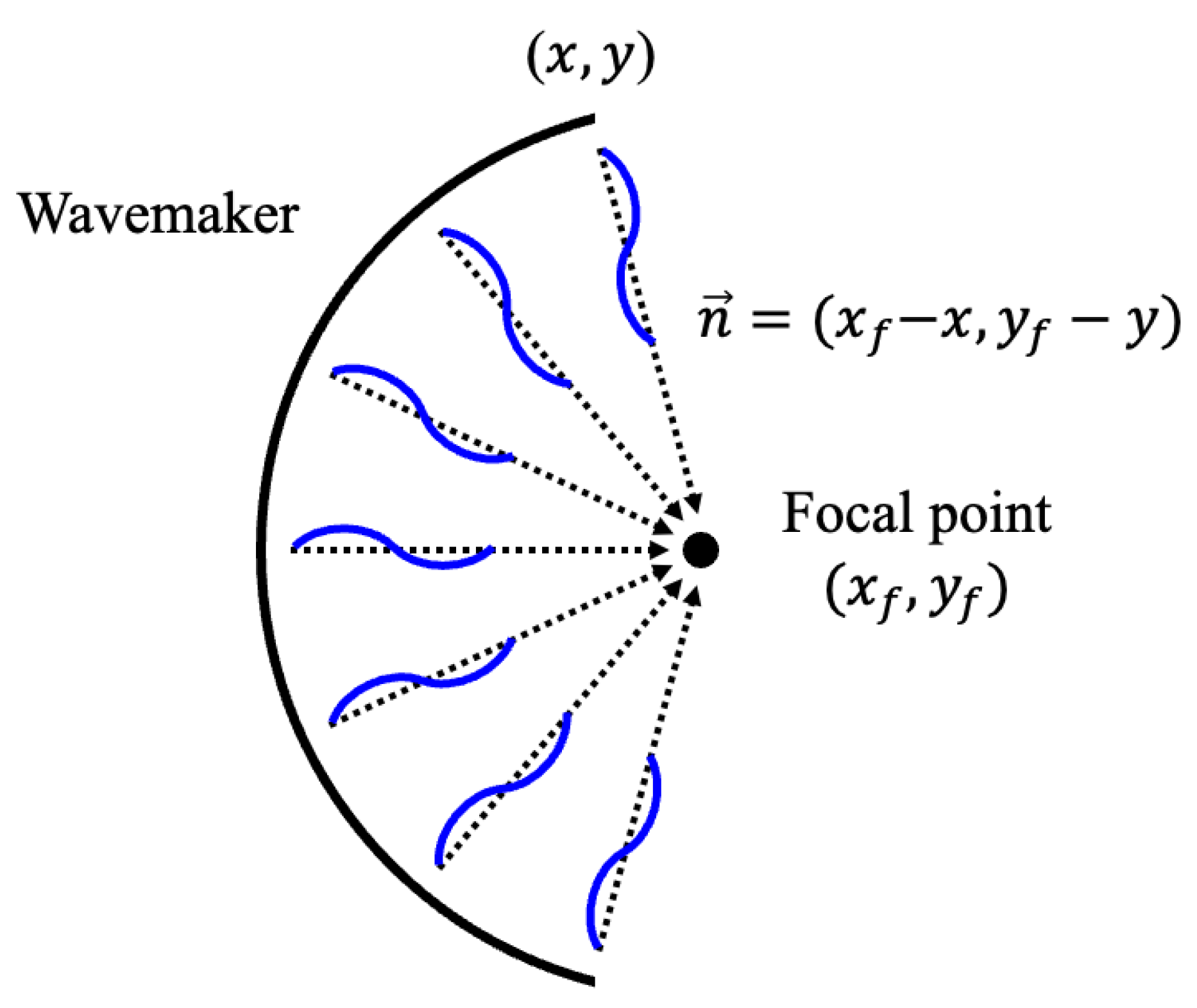
2.2. Wave Generation and Absorption
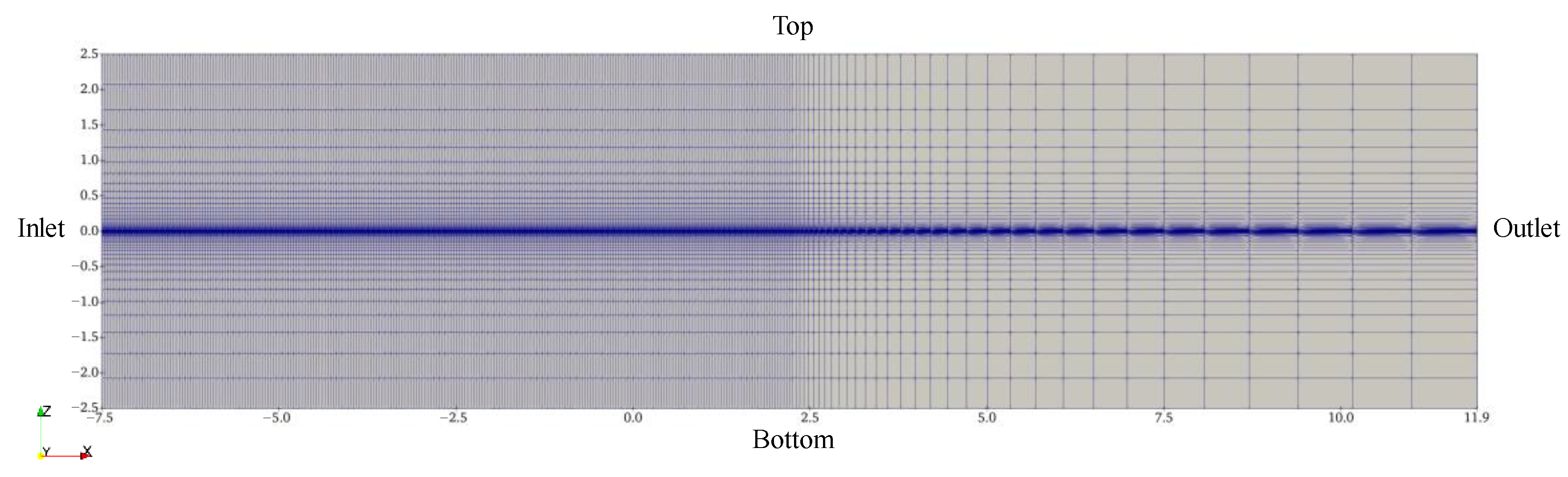
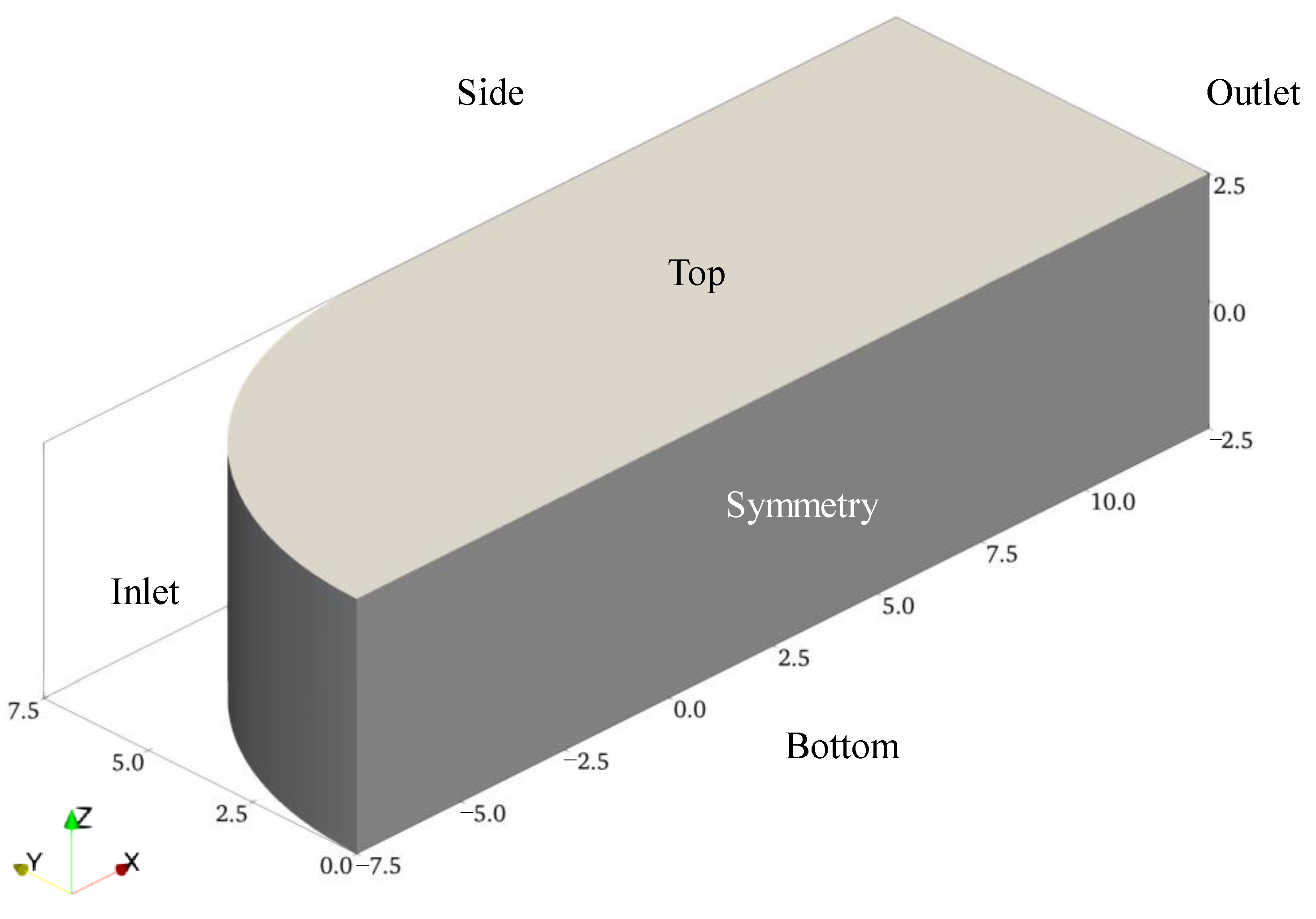
2.3. Numerical Methods
3. Results and Discussion
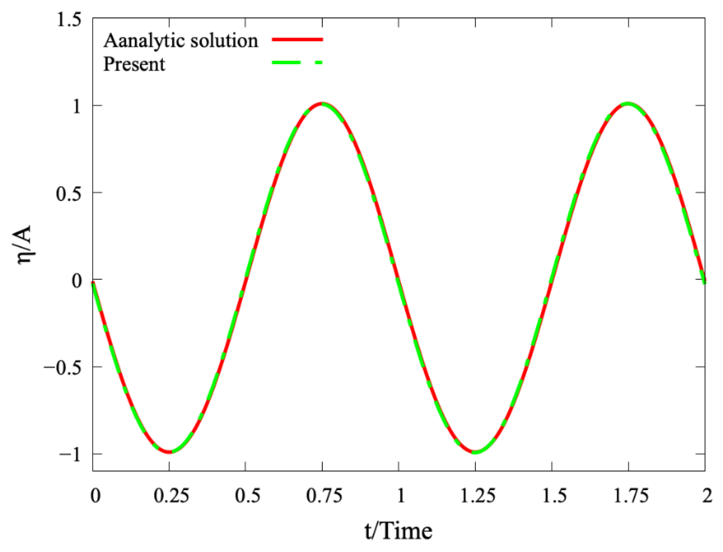
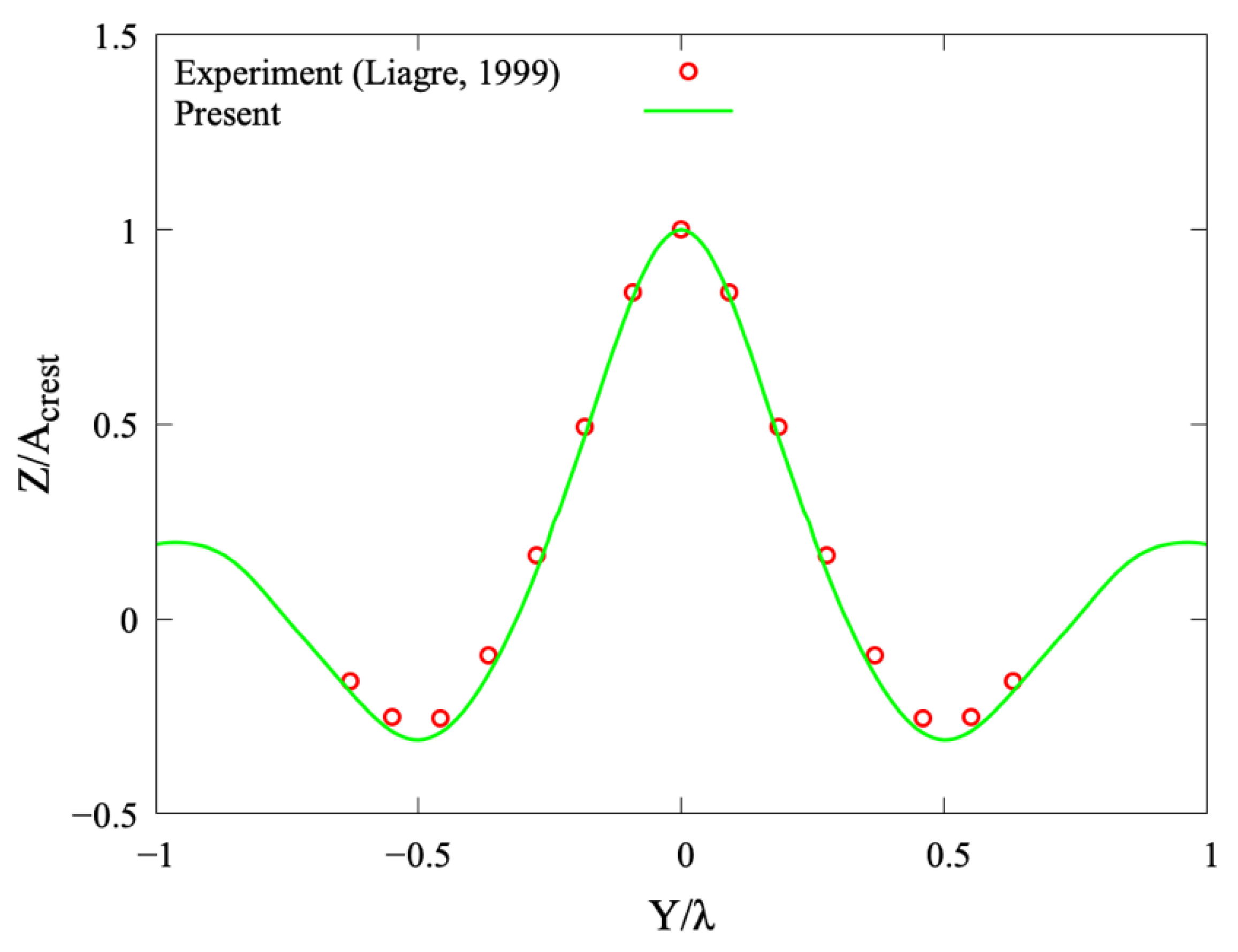
3.1. Regular Wave Simulation
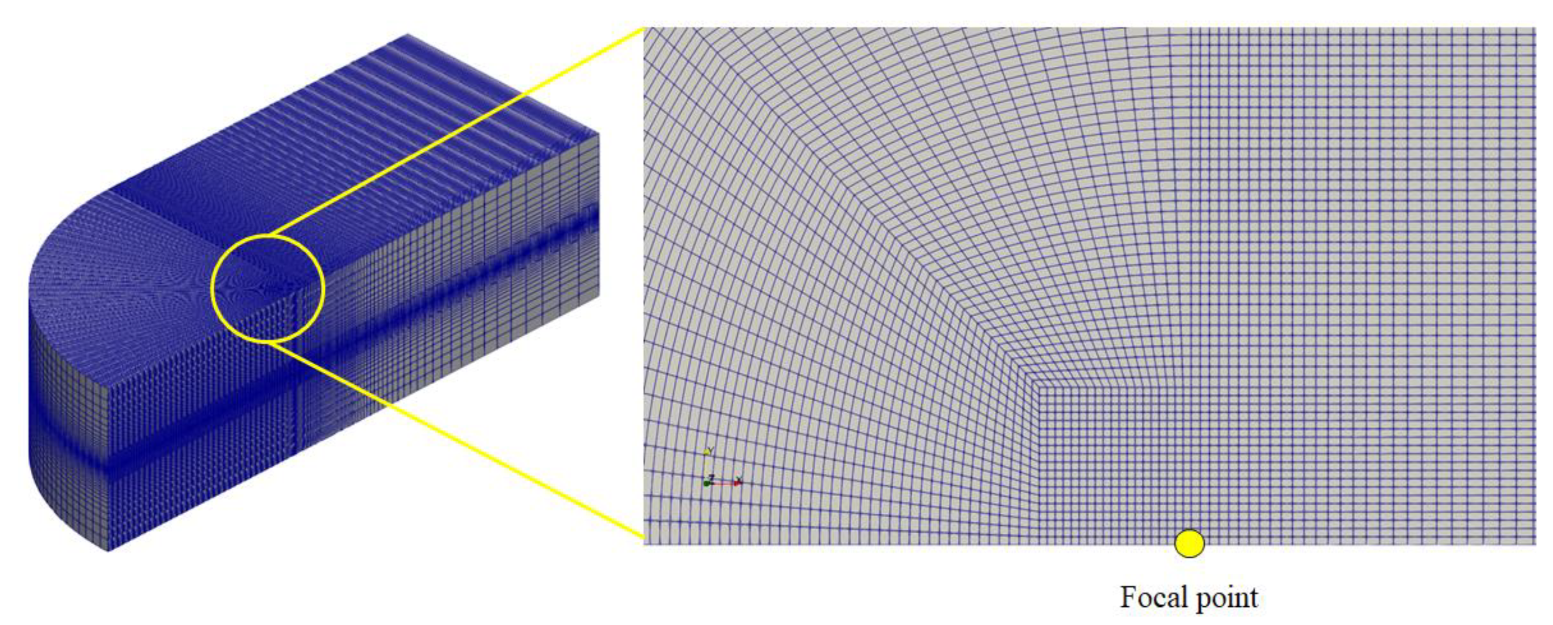
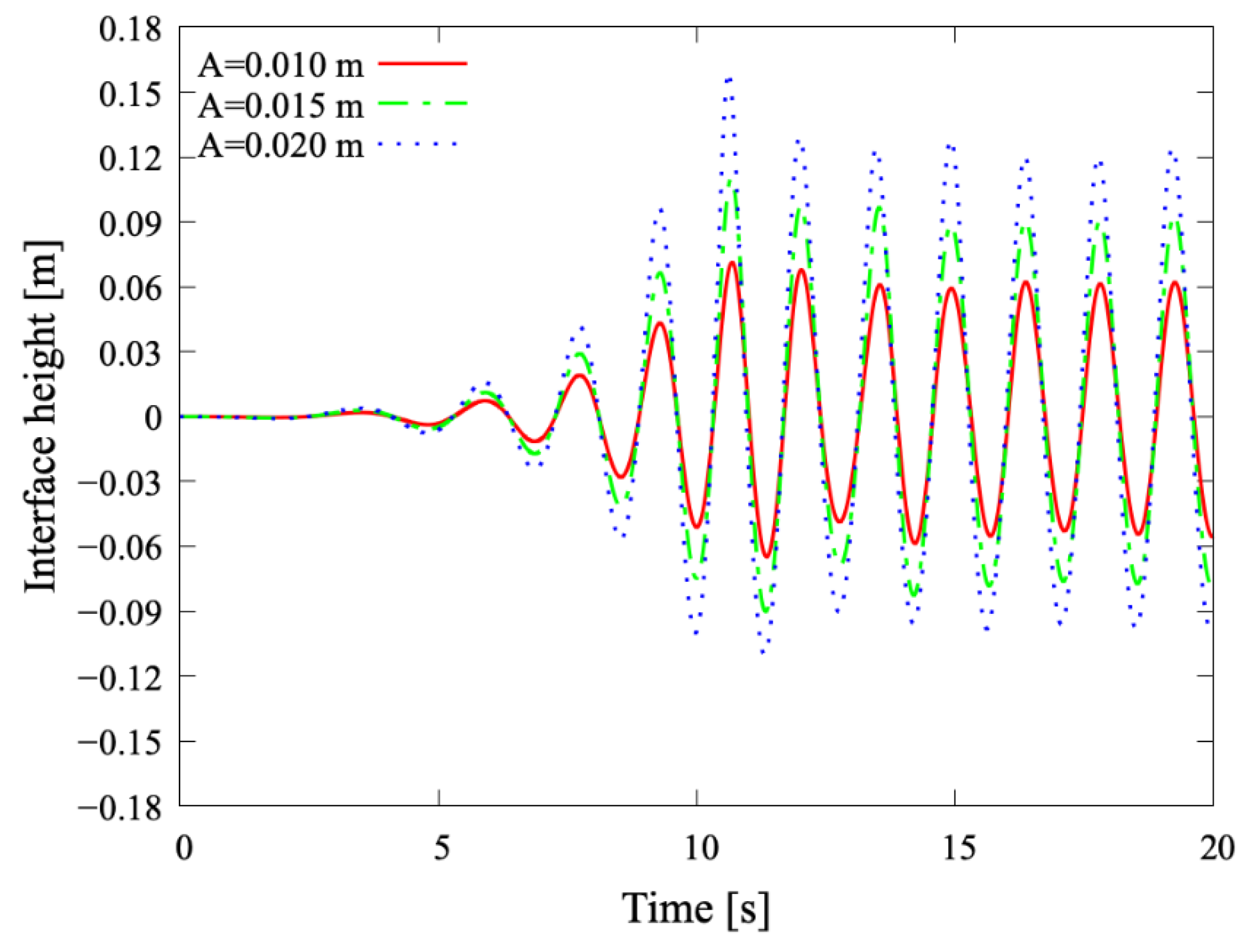
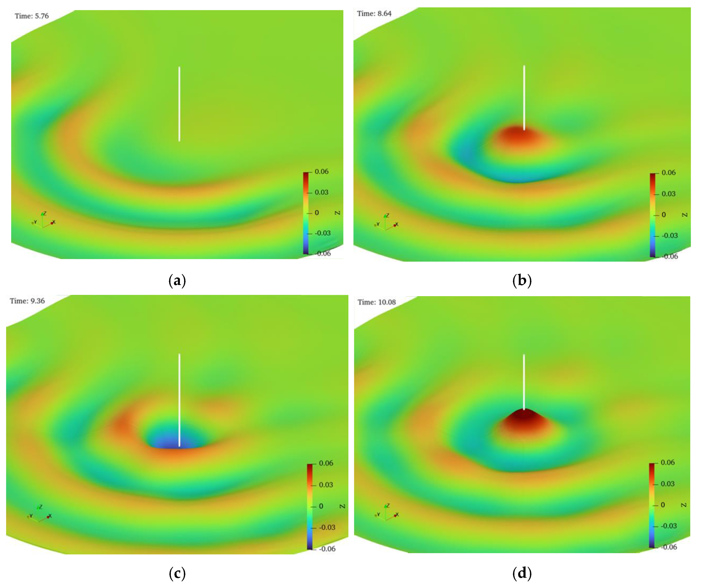
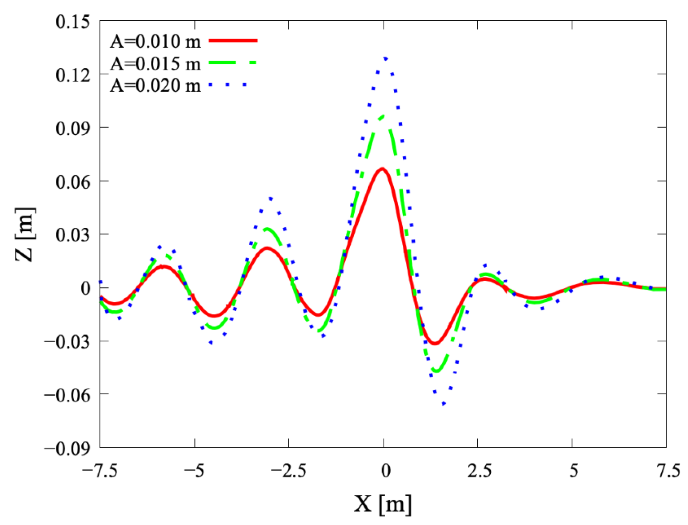
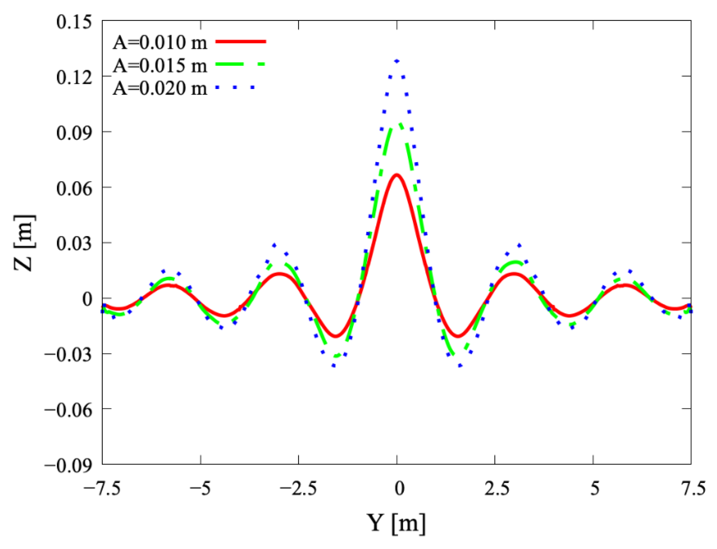
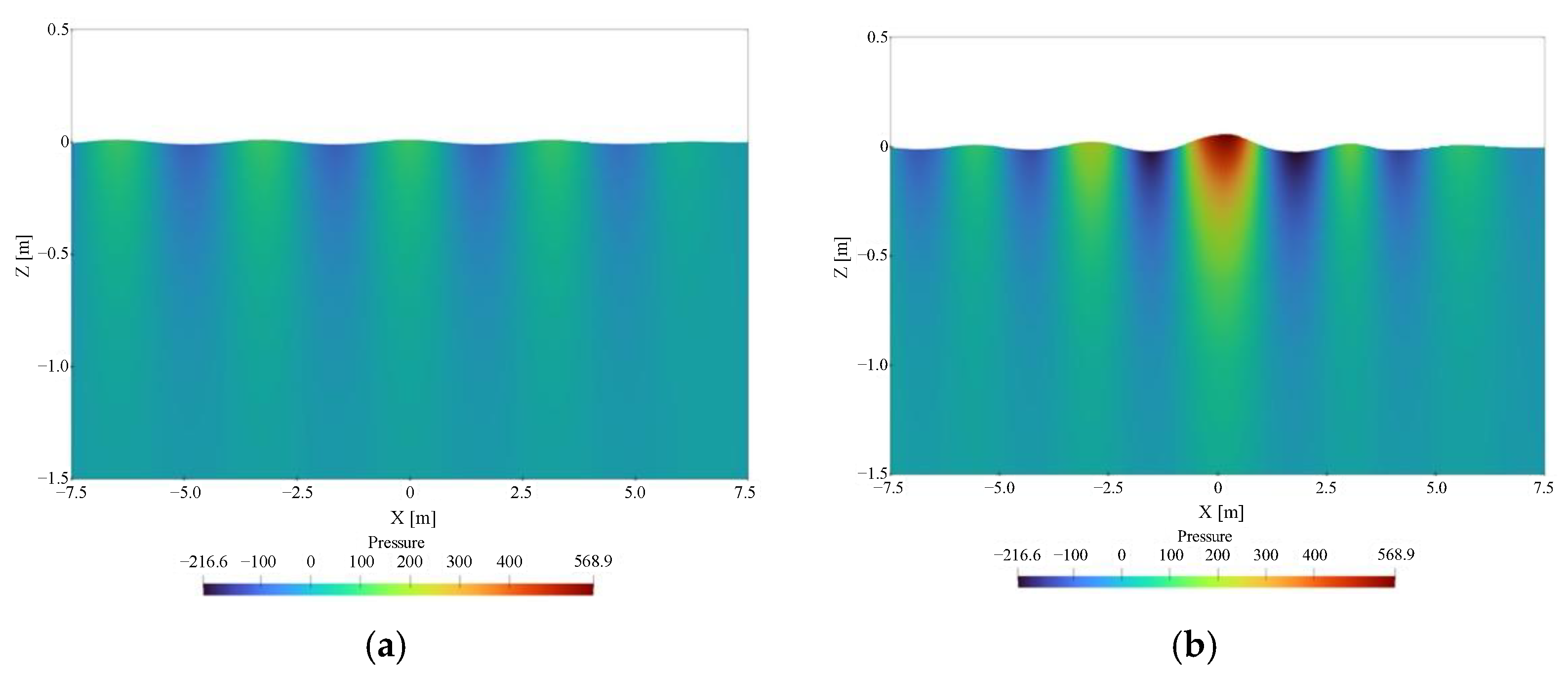
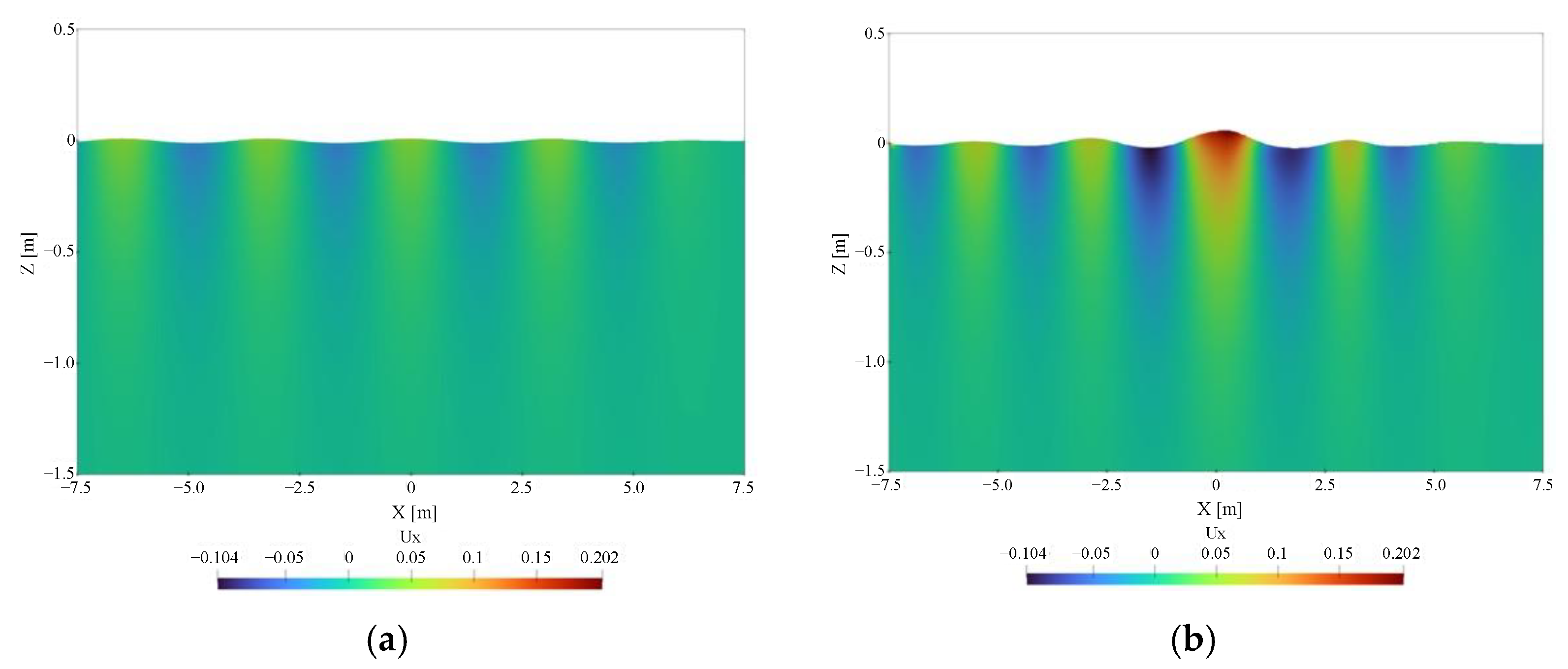
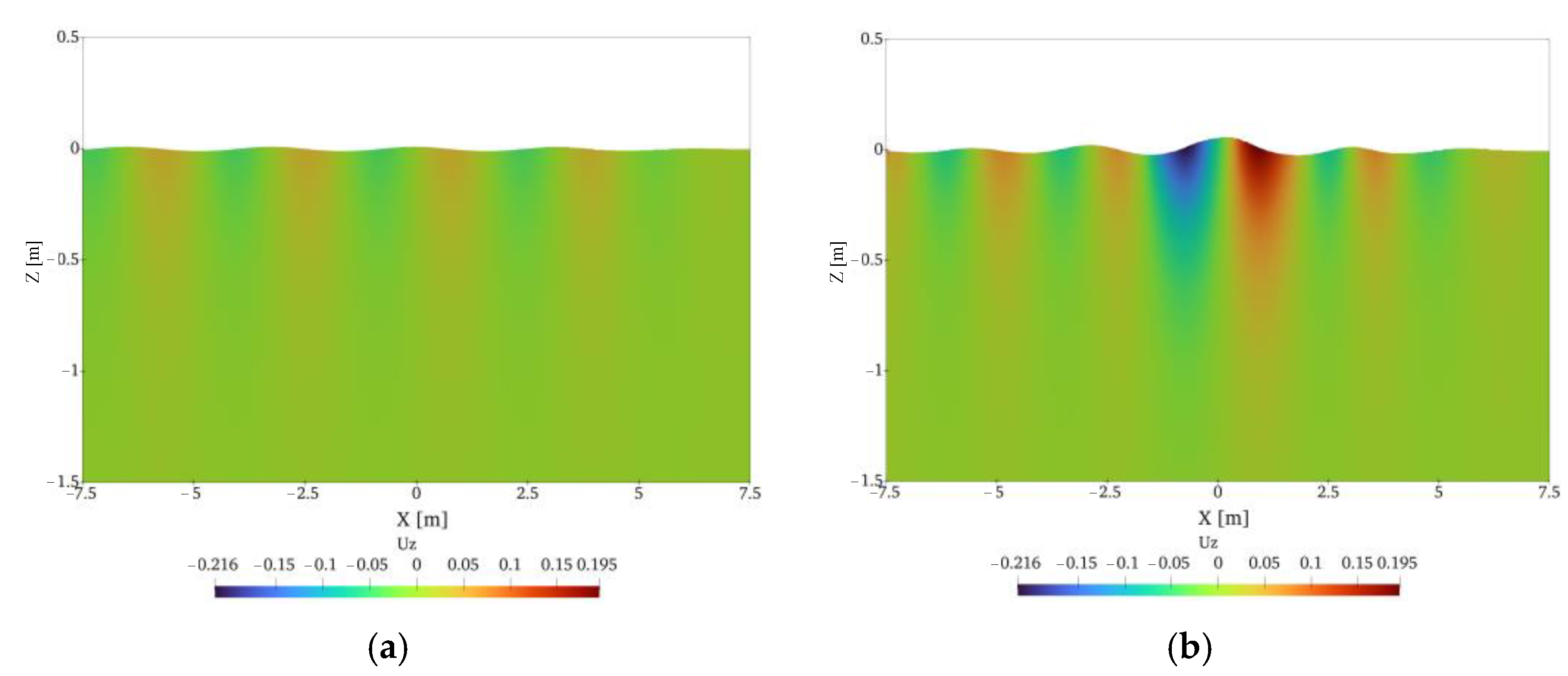
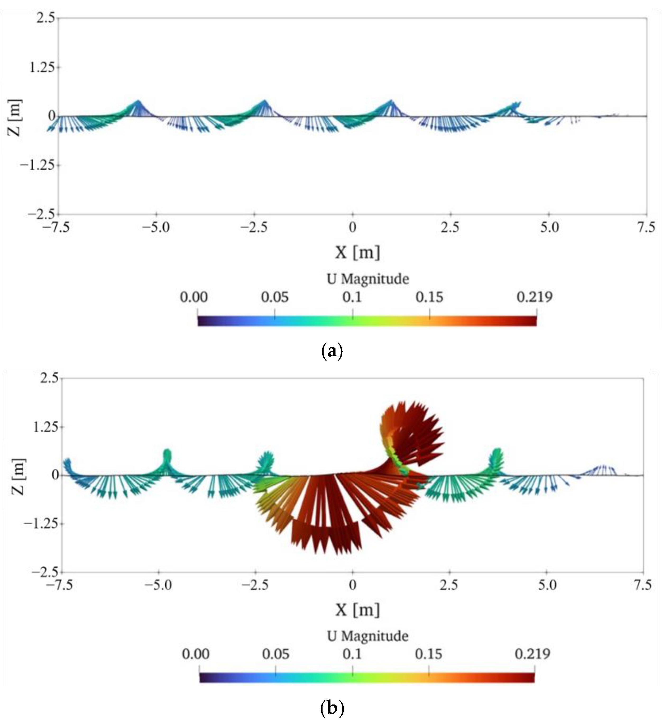
3.2. Bull’s-Eye Waves Simulation
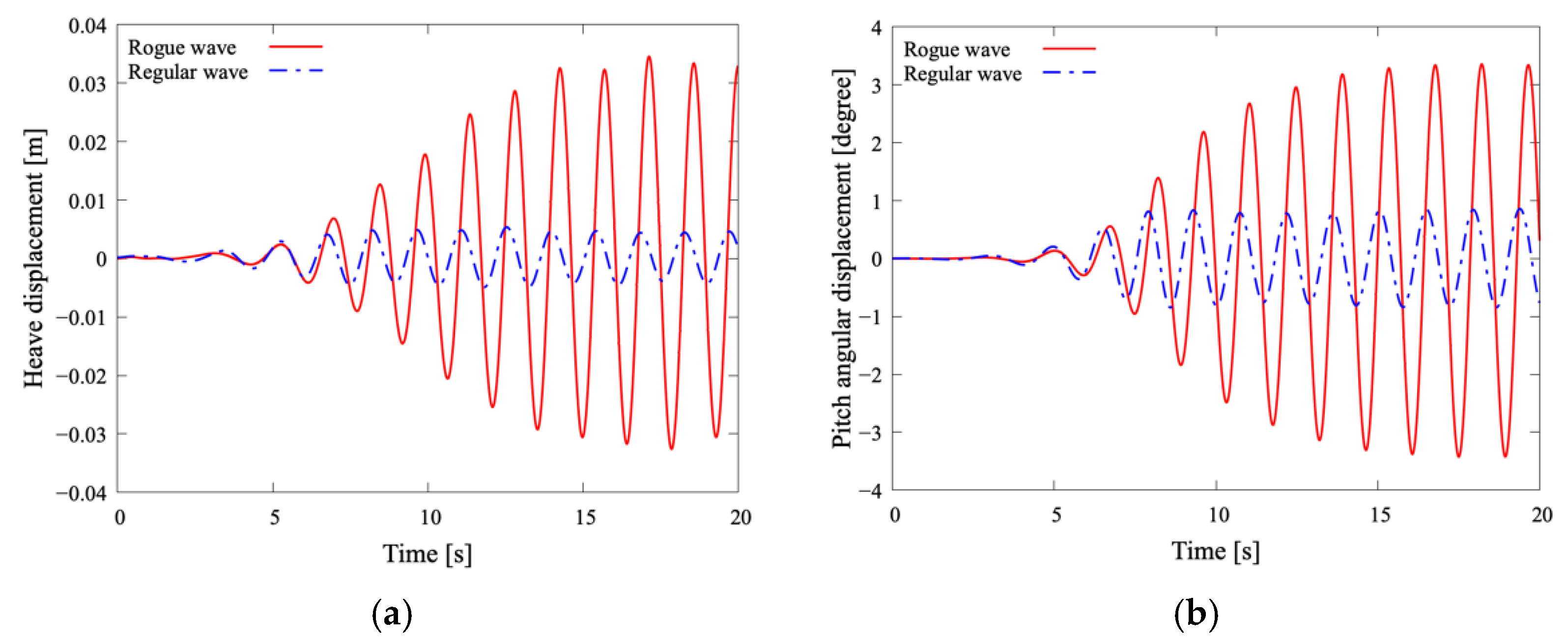
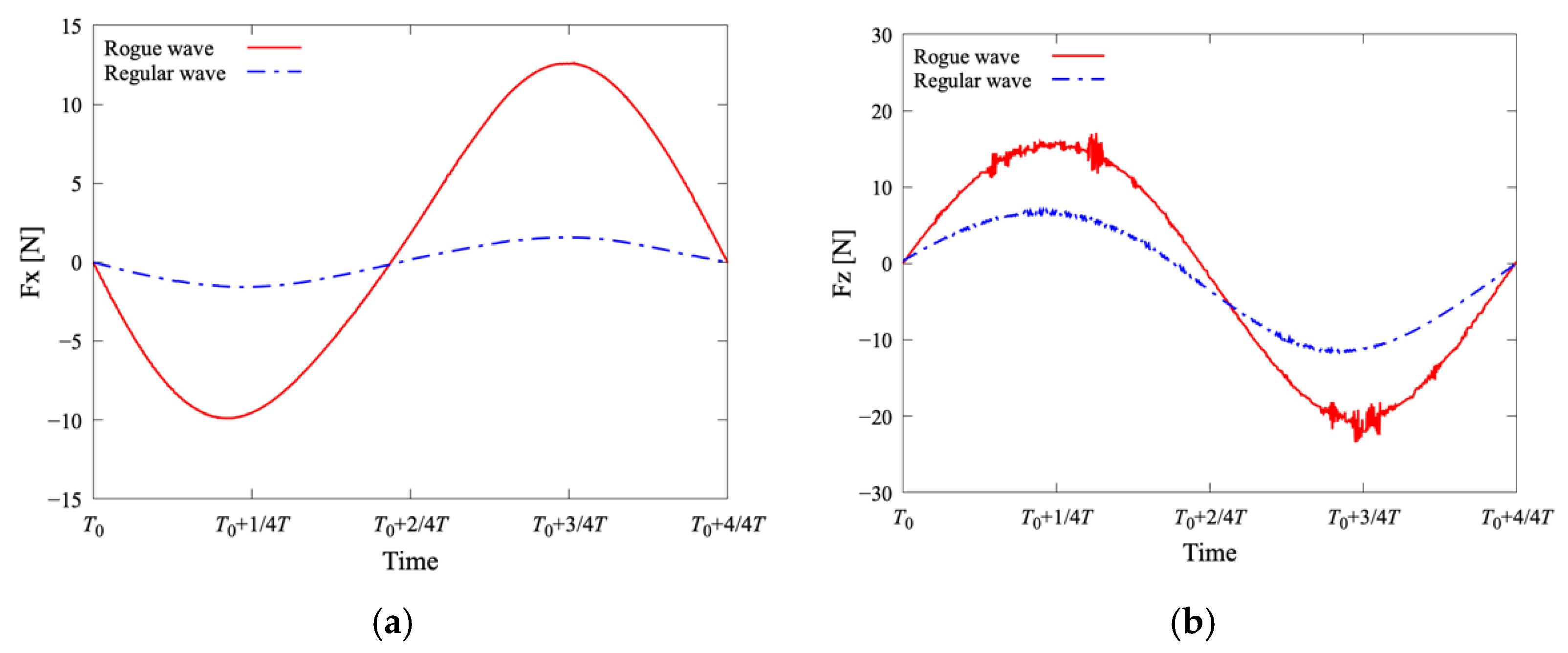
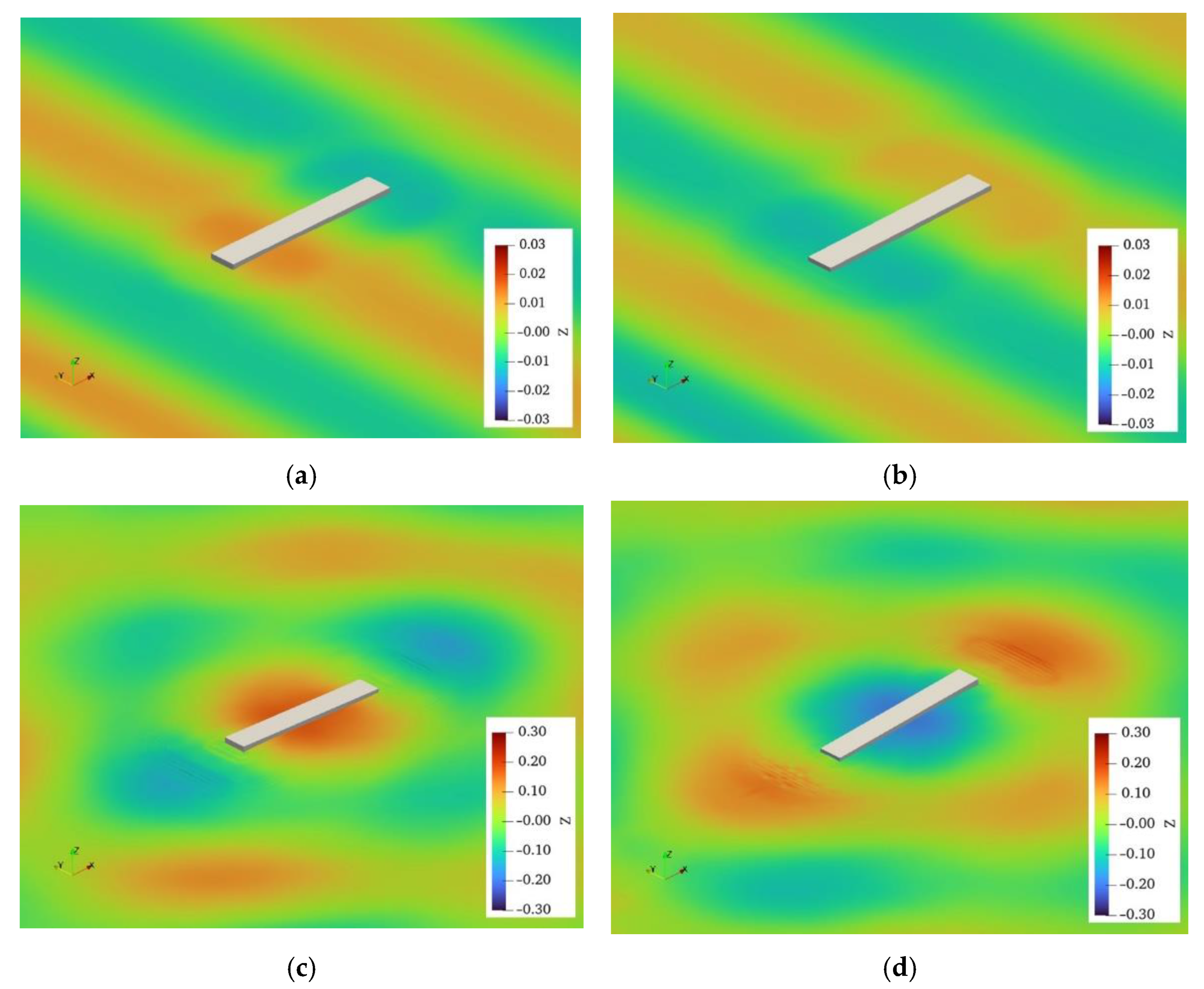
3.3. Response of Floating Body
4. Concluding Remarks
Author Contributions
Funding
Institutional Review Board Statement
Informed Consent Statement
Data Availability Statement
Conflicts of Interest
References
- Haver, S. A Possible Freak Wave Event Measured at the Draupner Jacket January 1 1995. In Proceedings of the Rogue Waves, Brest, France, 20–22 October 2004. [Google Scholar]
- Chabchoub, A.; Hoffmann, N.; Onorato, M.; Akhmediev, N. Super Rogue Waves: Observation of a Higher-Order Breather in Water Waves. Phys. Rev. X 2012, 2, 011015. [Google Scholar] [CrossRef]
- Peregrine, D.H. Water waves, nonlinear Schrödinger equations and their solutions. J. Aust. Math. Soc. Ser. B 1983, 25, 16–43. [Google Scholar] [CrossRef]
- Yuen, H.C.; Lake, B.M. Nonlinear deep water waves: Theory and experiment. Phys. Fluids 1975, 18, 956. [Google Scholar] [CrossRef]
- Lake, B.M.; Yuen, H.C.; Rungaldier, H.; Ferguson, W.E. Nonlinear deep-water waves: Theory and experiment. Part 2. Evolution of a continuous wave train. J. Fluid Mech. 1977, 83, 49–74. [Google Scholar] [CrossRef]
- Xiao, W.; Liu, Y.; Wu, G.; Yue, D.K.P. Rogue wave occurrence and dynamics by direct simulations of nonlinear wave-field evolution. J. Fluid Mech. 2013, 720, 357–392. [Google Scholar] [CrossRef]
- Rudman, M.; Cleary, P.W. Rogue wave impact on a tension leg platform: The effect of wave incidence angle and mooring line tension. Ocean Eng. 2013, 61, 123–138. [Google Scholar] [CrossRef]
- Rudman, M.; Cleary, P.W. The influence of mooring system in rogue wave impact on an offshore platform. Ocean Eng. 2016, 115, 168–181. [Google Scholar] [CrossRef]
- Hu, Z.; Tang, W.; Xue, H.; Zhang, X.; Wang, K. Numerical study of rogue wave overtopping with a fully-coupled fluid-structure interaction model. Ocean Eng. 2017, 138, 48–58. [Google Scholar] [CrossRef]
- Ha, Y.J.; Nam, B.N.; Kim, K.K.; Hong, S.Y. CFD simulations of wave impact loads on a truncated circular cylinder by breaking waves. Int. J. Offshore Polar Eng. 2019, 29, 306–314. [Google Scholar] [CrossRef]
- Alberello, A.; Pakodzi, C.; Nelli, F.; Bitner-Gregersen, E.M.; Toffoli, A. Three dimensional velocity field underneath a breaking rogue wave. In Proceedings of the International Conference on Offshore Mechanics and Artic Engineering, Trondheim, Norway, 25–30 June 2017. [Google Scholar]
- Ransley, E.J.; Greaves, D.; Raby, A.; Simmonds, D.; Hann, M. Survivability of wave energy converters using CFD. Renew. Energy 2017, 109, 235–247. [Google Scholar] [CrossRef]
- Dorozhko, V.M.; Bugaev, V.G.; Kitaev, M.V. CFD Simulation of an Extreme Wave Impact on a Ship. In Proceedings of the Twenty-Fifth International Ocean and Polar Engineering Conference, Kona, HI, USA, 25–26 June 2015. [Google Scholar]
- Chen, H.; Qian, L.; Bai, W.; Ma, Z.; Lin, Z.; Xue, M.A. Oblique focused wave group generation and interaction with a fixed FPSO-shaped body: 3D CFD simulations and comparison with experiments. Ocean Eng. 2019, 192, 106524. [Google Scholar] [CrossRef]
- Kim, H.; Park, S. Coupled level-set and volume of fluid (CLSVOF) solver for air lubrication method of a flat plate. J. Mar. Sci. Eng. 2021, 9, 231. [Google Scholar] [CrossRef]
- Dalrymple, R.A. Directional wavemaker theory with sidewall reflection. J. Hydraul. Res. 1985, 27, 23–34. [Google Scholar] [CrossRef]
- Park, S.; Park, S.W.; Rhee, S.H.; Lee, S.B.; Choi, J.-E.; Kang, S.H. Investigation on the wall function implementation for the prediction of ship resistance. Int. J. Nav. Archit. Ocean Eng. 2013, 5, 33–46. [Google Scholar] [CrossRef]
- Seo, S.; Park, S.; Koo, B.Y. Effect of wave periods on added resistance and motions of a ship in head sea simulations. Ocean Eng. 2017, 137, 309–327. [Google Scholar] [CrossRef]
- Lee, S.C.; Song, S.; Park, S. Two-way coupled solver between platform motions and mooring system for a moored floating platform. Processes 2021, 9, 1393. [Google Scholar] [CrossRef]
- Menter, F. Zonal Two Equation k-w Turbulence Models for Aerodynamic Flows. In Proceedings of the 23rd Fluid Dynamics Conference, Orlando, FL, USA, 6–9 July 1993. [Google Scholar]
- Weiss, J.M.; Maruszewski, J.P.; Smith, W.A. Implicit solution of preconditioned Navier-Stokes equations using algebraic multigrid. AIAA J. 1999, 37, 29–36. [Google Scholar] [CrossRef]
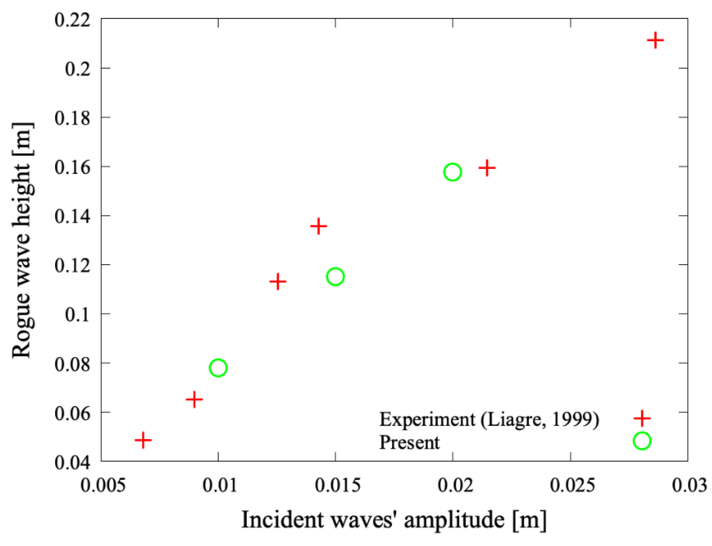
- Liagre, P.-Y.F.B. Generation and Analysis of Multi-Directional Waves. Master’s Thesis, Texas A&M University, College Station, TX, USA, 1999. [Google Scholar]


| Parameters | Value |
|---|---|
| ρwater | 998 kg/m3 |
| νwater | 1.004 × 10⁻⁶ m2/s |
| ρair | 1.204 kg/m3 |
| νair | 1.506 × 10⁻⁵ m2/s |
| 0.0445 m/s | |
| Rewave amplitude | 445 |
| Refloating body | 88,900 |
| Wave Height (H) | Wavelength (λ) | Wave Period (T) | |
|---|---|---|---|
| Wave condition 1 | 0.02 m | 3.2375 m | 1.44 s |
| Wave condition 2 | 0.03 m | ||
| Wave condition 3 | 0.04 m |
| Grid System | Number of Mesh in Wavelength/Wave Height | Total Number of Meshes | |
|---|---|---|---|
| Index | Description | ||
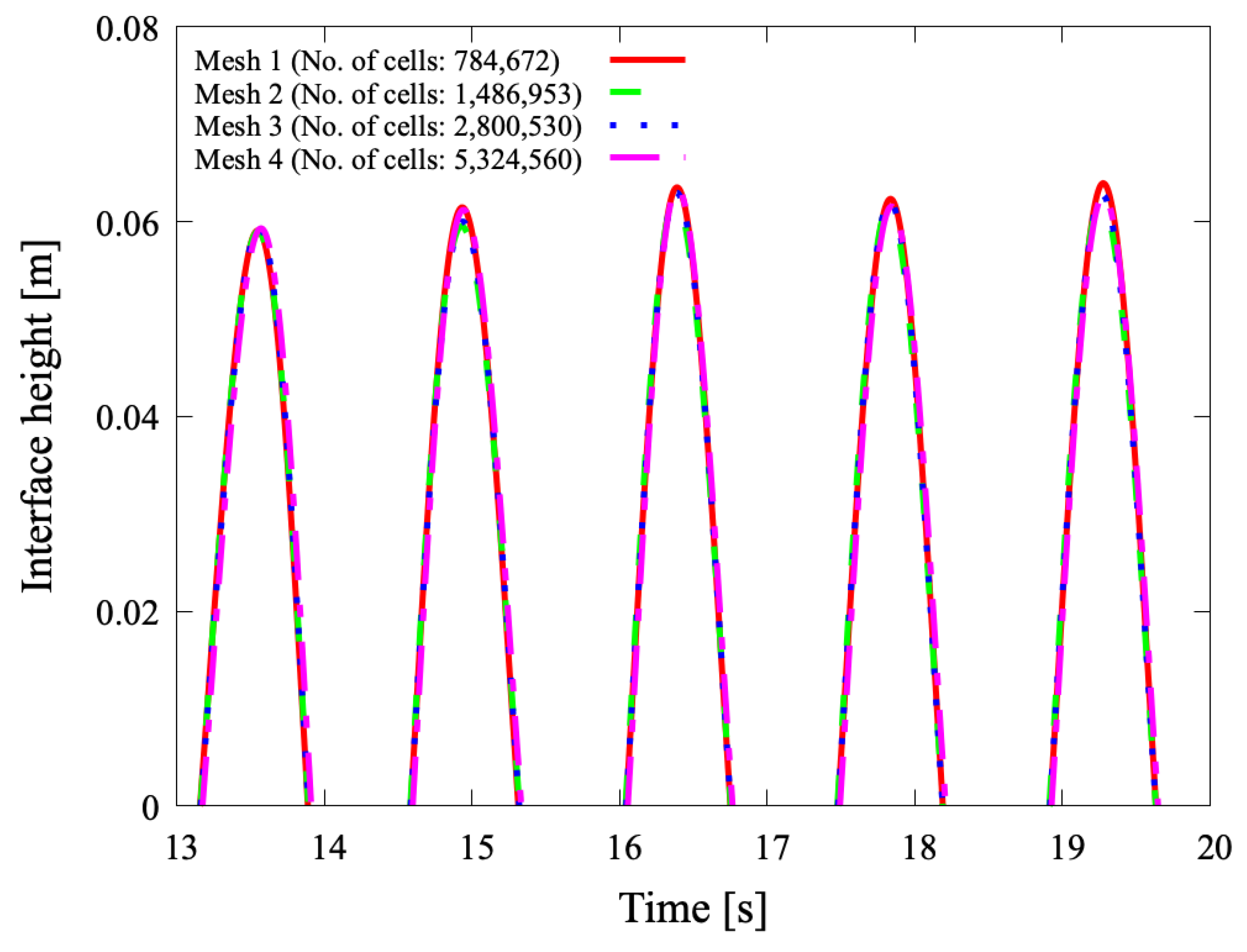
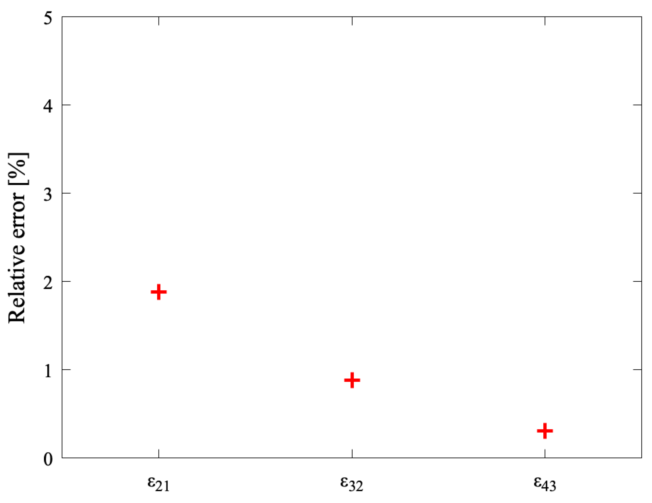
| 1 | Coarse mesh | 63/12 | 784,672 |
| 2 | Medium mesh | 80/16 | 1,486,953 |
| 3 | Fine mesh | 100/20 | 2,800,530 |
| 4 | Extra fine mesh | 126/24 | 5,324,560 |
| Wave Height (H) | Acrest/Atrough | Wave Height (H)/Wave Length (λ) | |
|---|---|---|---|
| Wave condition 1 | 0.02 m | 0.057/0.022 = 2.61 | 0.078/3.235 = 0.024 |
| Wave condition 2 | 0.03 m | 0.084/0.031 = 2.73 | 0.115/3.169 = 0.036 |
| Wave condition 3 | 0.04 m | 0.119/0.039 = 3.07 | 0.158/3.103 = 0.051 |
Publisher’s Note: MDPI stays neutral with regard to jurisdictional claims in published maps and institutional affiliations. |
© 2022 by the authors. Licensee MDPI, Basel, Switzerland. This article is an open access article distributed under the terms and conditions of the Creative Commons Attribution (CC BY) license (https://creativecommons.org/licenses/by/4.0/).
Share and Cite
Jeon, W.; Park, S.; Jeon, G.-M.; Park, J.-C. Computational Study on Rogue Wave and Its Application to a Floating Body. Appl. Sci. 2022, 12, 2853. https://doi.org/10.3390/app12062853
Jeon W, Park S, Jeon G-M, Park J-C. Computational Study on Rogue Wave and Its Application to a Floating Body. Applied Sciences. 2022; 12(6):2853. https://doi.org/10.3390/app12062853
Chicago/Turabian StyleJeon, Wooyoung, Sunho Park, Gyu-Mok Jeon, and Jong-Chun Park. 2022. "Computational Study on Rogue Wave and Its Application to a Floating Body" Applied Sciences 12, no. 6: 2853. https://doi.org/10.3390/app12062853
APA StyleJeon, W., Park, S., Jeon, G.-M., & Park, J.-C. (2022). Computational Study on Rogue Wave and Its Application to a Floating Body. Applied Sciences, 12(6), 2853. https://doi.org/10.3390/app12062853