Predicting the Fire Source Location by Using the Pipe Hole Network in Aspirating Smoke Detection System

Abstract

The aspirating smoke detector (ASD) is one of the most critical pieces of equipment for detecting smoke in a protected area when a fire occurs. It has more advantages than a conventional smoke detector because it can be used in extreme conditions, such as cold storage facilities or hot aisle containment areas. ASD uses a fan to draw air from the protected area into the pipe network system via pipe holes. The sucked air is transported into the sensing chamber to detect smoke. If the obscuration in the sensing chamber is greater than the setpoint, the ASD will sound an alarm so that people realize there is a fire. For this reason, investigating the effect of the pipe hole network on obscuration in the ASD is critical. In this study, a Pipe Hole Network Program was developed to consider the pipe flow parameter. A numerical study based on the program and an experimental study was performed. The results showed that the numerical results had the same trend as the experimental study. The further the location of the fire source was, the lower the obscuration was. In addition, the correlation between the obscuration parameter and the fire source distance was also derived. It could be used to predict the fire source location in the aspirating smoke detection system.

1. Introduction

A smoke detection system is one of the most critical pieces of equipment for detecting smoke early to reduce the danger of fire, as well as to reduce human casualties. A conventional smoke detector detects smoke from an incipient fire and triggers an alarm system. However, it has some specific problems. In extreme temperature environments, such as a cold warehouse or a hot aisle area, a conventional smoke detection system cannot be applied. In the cold warehouse, high-bay storage can affect the airflow and obstruct the detection and response to a fire event. Besides, the operating temperatures typically range between 8 °C to −40 °C resulting in cold storage environments exhibiting harsh climatic conditions. These extreme temperatures of refrigerated storage facilities are a primary challenge to detecting a cold store fire as most forms of conventional smoke detection are not designed to operate in harsh climatic environments. In addition, high airflows created by blast chiller units and condensation can impede the operation of conventional passive detectors too. For this reason, the aspirating smoke detector (ASD) system has been developed to detect smoke. ASD uses a pipe hole network to draw air from protected areas to the sensing chamber, so it has a quick response. At the sensing chamber, air samples are illuminated with a high intensity light source, which causes smoke particles to reflect light to a solid-state photoreceiver. At the detector, an analog signal is generated to the control unit, which displays the smoke obscuration sensitivity. The two main advantages of the ASD system are the use of the sensitivity setting for incipient fire detection and one ASD system can cover large areas by using the piping network. For the above reasons, research regarding aspirating smoke detection systems and pipe hole networks should be conducted to enhance the efficiency of the system as well as to reduce the transport time of smoke.

There are many kinds of research relating to this system. Cheng et al. [1] performed a simulation of a sampling pipe hole network with an ASD. They also compared the values between numerical and experimental studies. In that paper, a mathematical model was built to apply a theory to calculate the flow rate and transport time. The results showed that the values from the mathematical model were in accordance with the experiment values. Furthermore, the pipe network has been investigated in many other systems in addition to aspirating smoke detection.

Carello et al. [2] investigated the pressure drop in pipelines for pneumatic systems. In that paper, a theoretical analysis was compared with an experimental study. The various upstream pressure and different internal diameters are also used to evaluate the pressure drop in the pipe system. The results showed that the experimental study and theoretical analysis were in good agreement.

Nowadays, with the development of technology, numerical studies can also be applied to calculate the pressure loss in the pipe network. Essienubong et al. [3] carried out a pressure loss analysis of air duct flow using Computational Fluid Dynamics (CFD). They determined the pressure loss in air ducts by hand calculation and computer simulation. The velocity in the pipe changed from 5 m/s to 10, 20, and 40 m/s, respectively. When the velocity increased, the pressure loss also increased. The results obtained from hand calculations and simulations were almost the same. Besides, Gajbhiye et al. [4] and Perumal et al. [5] have considered the pressure loss coefficient of pipe fittings by CFD. The results were conclusive that a validated CFD model was a cheap and reliable tool for loss coefficient estimation of pipe fitting and complex fluid flow.

Singh RK [6] investigated the airflow in a network used in aspirated smoke detectors. The numerical and experimental study on the flow was carried out in this research. The CFD results were analyzed and compared with the commonly accepted values of the local coefficient of the sampling hole and friction factor. The disturbances occurred because of the jet flows from the sampling holes. Gai et al. [7] have performed an analytical and experimental study on complex compressed air pipe networks. They applied a matrix to describe the topology structure of the compressed airflow. Then, the relationship between the pressure and the flow of air was derived, and a prediction method of pressure fluctuation and airflow was proposed. The predicted results had the right consistency in the experimental data.

In addition, Huang et al. [8,9] have considered the smoke spread process in large-space buildings with various heights by using the Fire Dynamics Simulator (FDS). In that study, the fire source location was in the center of the room. Besides, twelve aspirator samplers were used in the ASD system. They were divided into three groups, group 1 and group 3 were located at the edge of the building. Group 2 was located at the centerline. The results showed that as the aspirator samplers were located nearby to the building’s edge, the alarm for the fire was faster. So, the obscuration of the ASD was affected by the building’s edge. Zhenna et al. [10] also investigated the performance study of fire alarm systems in large space buildings. The study showed that the numerical calculation can forecast the response time for the ASD system very well and can be applied as a guide for designing an ASD system in large space buildings. Furthermore, many studies relating airflow, fires, and smoke detectors have been carried out and are described in the literature. The flow pressure analysis of pipe networks with linear theory method [11], modeling airflow in a prototype sanitary sewer system [12], and prediction of fan-assisted flow in a pipe network [13] have been investigated. Besides, the efficient iterative method for looped pipe networks [14] and the flow analysis in aspirating smoke detectors [15] speed was studied by changing airspeed. The airflow rate measurement with the differential pressure method [16] and experimental of turbulent flow through an orifice [17] has been considered. The study showed the turbulent flow through the orifice is a function of the orifice geometry. Moreover, based on the fire spread in the warehouse [18,19] as well as fire safety management [20], the study of fire detection systems, such as aspirator smoke detectors for warehouses and large space buildings [21,22,23,24,25] have been performed.

Although there are many papers regarding the pressure drop in the pipe and the obscuration in larger-space buildings, there has been no research relating to predicting the fire source location by using the pipe hole network in the aspirating smoke detector. For this reason, the Pipe Hole Network Program was developed to calculate the parameters of the pipe network. Based on the program, a numerical study and an experimental study were carried out to calculate the parameters to predict the fire source location when a fire occurs.

2. Theoretical Analysis

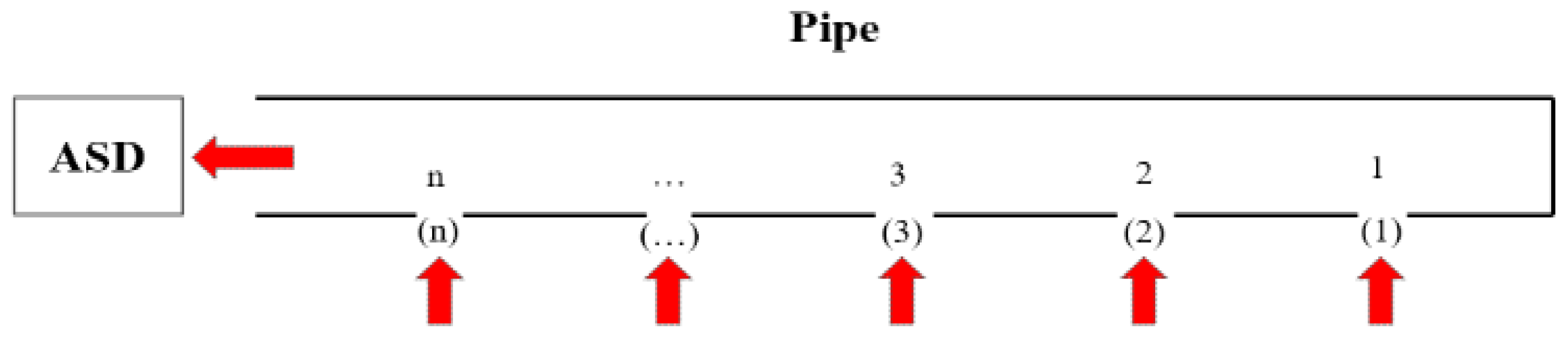
2.1. Pressure Drop in the Pipe Network

As the fluid flows through the pipe network, the pressure changes because a pressure drop occurs in the pipe system. This may be caused by friction between the fluid in the pipe and the pipe wall. Moreover, when the fluid flows through any pipe fittings, bends, valves, or components, there is a minor loss in pressure at these fittings. For the above reasons, the pressure drop in the pipe generally includes major losses and minor losses.

To calculate friction loss in a pipe which is known as the Darcy–Weisbach equation or the Darcy–Weisbach formula is issued:

$$h_l=f\frac{L}{D}\frac{V^2}{2}\mathsf{\rho }$$

(1)

where h_l is a head loss, f is a friction factor, L is the length of the pipework (m), D is the inner diameter of the pipework (m), V is the velocity (m/s), and ρ is the density of the fluid.

When the Reynolds number is smaller than 2280, the following equation is applied to calculate the friction coefficient:

$$f=\frac{64}{Re} \mathrm{if} Re < 2280$$

(2)

Moreover, Cole [26] determined the relationship between the friction factor and Reynolds number when Re > 2280. It depends on the regimes of the flow as shown by the following equations:

$$f=0.028 \mathrm{if} 2280 < Re < 2400$$

(3)

$$f=0.028+0.007(Re-2400)/600 \mathrm{if} 2400 < Re < 3000$$

(4)

$$f= 0.035+0.004(Re-3000)/800 \mathrm{if} 3000 < Re < 4400$$

(5)

To determine the pipe friction coefficient when the flow is turbulent, the Colebrook Equation [27] was used as shown in the following equation:

$$\frac{1}{f^{0.5}}=-2.0\log \left(\frac{e/D}{3.7}+\frac{2.51}{Re\times f^{0.5}}\right)$$

(6)

where f is the pipe friction coefficient, e is the roughness, D is the diameter of the pipe, and Re is the Reynolds number

In the pipe, the above friction factor can be applied where there are no jet disturbances. When the disturbances occurred because of the jet flows from the sampling holes, the correction friction factor from Singh RK [6] was applied.

In addition to the major loss, the minor loss is critical to evaluate the pressure drop in the pipe network. The pipe fittings, valves, and bends are considered when calculating the minor loss. There are some associated K factors or local loss coefficients that are used to calculate the minor loss. These coefficients allow the calculation of the pressure loss through the fitting for a particular fluid flowing at a specified velocity. Manufacturers of pipe fittings and valves often publish a fitting’s associated “K” factor. The following equation can be used to calculate the minor loss:

$$h_{lm}=K\frac{V^2}{2}\mathsf{\rho }$$

(7)

where K is generally the manufacturer’s published factor, V is the velocity, and ρ is the density of the fluid.

2.2. Obscuration

In the ASD system, obscuration is one of the most important parameters in supplying the signal for the fire alarm control system. It is a unit of measurement that specifies the smoke detector sensitivity. If there is smoke, the light intensity will decrease. The obscuration is expressed as the percent absorption per unit length. The higher the concentration of smoke, the higher the obscuration level. When a fire occurs, the smoke moves from the fire source through the pipe hole network to the ASD system. If the obscuration in the ASD is over the set value, the fire alarm sounds. In the aspirating smoke detection system, the value of obscuration can be calculated by the following equation [28]:

$$Obscuration=\left(1-exp\left(-K_m\frac{{\sum }_{i=1}^N{\mathsf{\rho }}_{s,i}\left(t-t_{d,i}\right)\dot{m_i}}{{\sum }_{i=1}^N\dot{m_i}}\right)\right)\times 100\%/m$$

(8)

where ${\dot{m}}_i$ is the mass flow rate at sampling location i, ${\mathsf{\rho }}_{s,i}$ is the soot density at sampling location i, t_d,i is the prior (delay) at the current time t, and K_m is the mass extinction coefficient associated with visible light.

3. Numerical and Experimental Studies

3.1. Numerical Study

3.1.1. Mathematical Model

To make a mathematical model, the sketch of the pipe hole shown in the Figure 1 was used.

Firstly, node (1) was considered. At this node, the concentration of smoke can be calculated by the following equations:

$$C_{(1)}=\frac{V_{(1),S}}{V_{(1),t}}$$

(9)

$$V_{1,t}=V_{(1),t};V_{1,s}=V_{(1),s}$$

(10)

$$C_1=\frac{V_{1,s}}{V_{1,t}}=\frac{V_{(1),s}}{V_{(1),t}}=C_{(1)}$$

(11)

where V_(1),s is the flow rate of the smoke in the air, V_(1),t is the total flow rate of smoke and air, and C₍₁₎ is the concentration of smoke through the pipe hole (1). Note that location 1 is inside the pipe at the first hole, and location (1) is outside at the first hole.

Similarly, the concentration at node (2) can be calculated by the same method:

$$C_{(2)}=\frac{V_{(2),S}}{V_{(2),t}}$$

(12)

$$V_{2,t}=V_{(2),t}+V_{1,t};V_{2,s}=V_{2,s}+V_{1,s}$$

(13)

$$C_2=\frac{V_{2,s}}{V_{2,t}}=\frac{V_{(2),s}+V_{1,s}}{V_{(2),t}+V_{1,t}}=\frac{C_{(2)}\times V_{(2),t}+C_1\times V_{(1),t}}{V_{(2),t}+V_{(1),t}}$$

(14)

Using the above reasons, the concentration at node (n) can be calculated:

$$C_n=\frac{V_{n,s}}{V_{n,t}}=\frac{V_{(n),s}+V_{n-1,s}}{V_{(n),t}+V_{n-1,t}}=\frac{C_{(n)}\times V_{(n),t}+C_{n-1}\times V_{(n-1),t}}{V_{(n),t}+V_{(n-1),t}}$$

(15)

Besides, the smoke concentration is proportional with smoke particle size [29,30] by the following equation:

$$\frac{OD}{\ell } \infty C_s$$

(16)

where OD is the optical density, $\ell$ is path length, and $C_s$ is the smoke concentration at a given time.

Besides, the smoke concentration is related to the smoke number density as shown in the equation:

$$C_s\infty {\displaystyle \sum }{n}_i{d}_i{}^3$$

(17)

where $n_i$ and $d_i$ are the number count (density) and particle diameter for a given particle size i. Thus, a relationship between optical density per path length and the number count at a given time may be established as in the equation:

$$\frac{OD}{\ell } \infty {\displaystyle \sum }{n}_i{d}_i{}^3$$

(18)

And the optical density (OD) and obscuration (OBS) can be related by:

$$OBS=100\left[1-{10}^{-OD}\right]$$

(19)

Because the smoke concentration is proportional to the smoke obscuration and the smoke concentration is not easy to measure directly, thus the smoke obscuration has been investigated instead in the experiment.

To calculate the pressure drop in this system, the pressure value at every point needs to be determined. The pressure difference between the two points was determined by the pressure drop, which was calculated by the function of the friction factor, roughness and Reynolds number; the following equations were obtained:

$$P_1=P_{(1)}+\Delta P_{(1)\_1}$$

(20)

$$P_n=P_{(n)}+\Delta P_{(n)\_n}=P_{n-1}+\Delta P_{n-1\_n}$$

(21)

where $\Delta P_{\left(1\right)\_1}$ is the pressure drop that occurs at hole 1. Point (1) is the outside location at the first hole and point 1 is the inside location at the first hole.

In the pipe network, the main flow in the pipe can be affected by the high velocity outside flow through the hole. In that region, jet disturbances can exist. Singh RK [6] has investigated the effect of the jet disturbance at that region, and the correction friction factor has been applied. The correction friction factor is proportional to the correction disturbance ratio (Q_in/Q). Where Q_in is the flow rate of the fluid through the hole, and Q is the flow rate of the main flow in the pipe. Based on the above theoretical analysis, the Pipe Hole Network Program was developed to calculate the pressure drop, transport time, and obscuration of smoke for a real case.

3.1.2. Numerical Setup

In order to investigate the effect of pipe flow on the obscuration in aspirating smoke detection systems, different numerical case studies have been investigated. Firstly, the pipe with a length of 20 m and ten holes was considered. Then, the pipe with 20 m and twenty holes pipe was also investigated. The detailed information of case studies was shown as follows.

1.

ASD system with one branch pipe with ten holes.

Based on the Pipe Hole Network Program, the parameter of fluid flow in the pipe can be calculated. As the first step, a straight pipe with a length of 20 m was considered to investigate the flow in the ASD system. The pipe had 10 holes. The diameter of the hole was 5 mm. The specifications of the pipe are shown in

Table 1. Case study for the straight pipe with ten holes.

Hole	Distance from Hole to ASD 1 (m)	Hole Diameter (mm)	Hole Distance (m)
1	2	5	2
2	4	5	2
3	6	5	2
4	8	5	2
5	10	5	2
6	12	5	2
7	14	5	2
8	16	5	2
9	18	5	2
10	20	5	2

.

2.

ASD system with one branch pipe with twenty holes.

In this case, the pipe with a length of 20 m was considered to investigate the flow in the ASD system. The pipe had 20 holes. The parameters of the are shown in the

Table 2. Case study for the straight pipe with twenty holes.

Hole	Distance from Hole to ASD 1 (m)	Hole Diameter (mm)	Hole Distance (m)
1	1	5	1
2	2	5	1
3	3	5	1
4	4	5	1
…	…	…	…
16	16	5	1
17	17	5	1
18	18	5	1
19	19	5	1
20	20	5	1

.

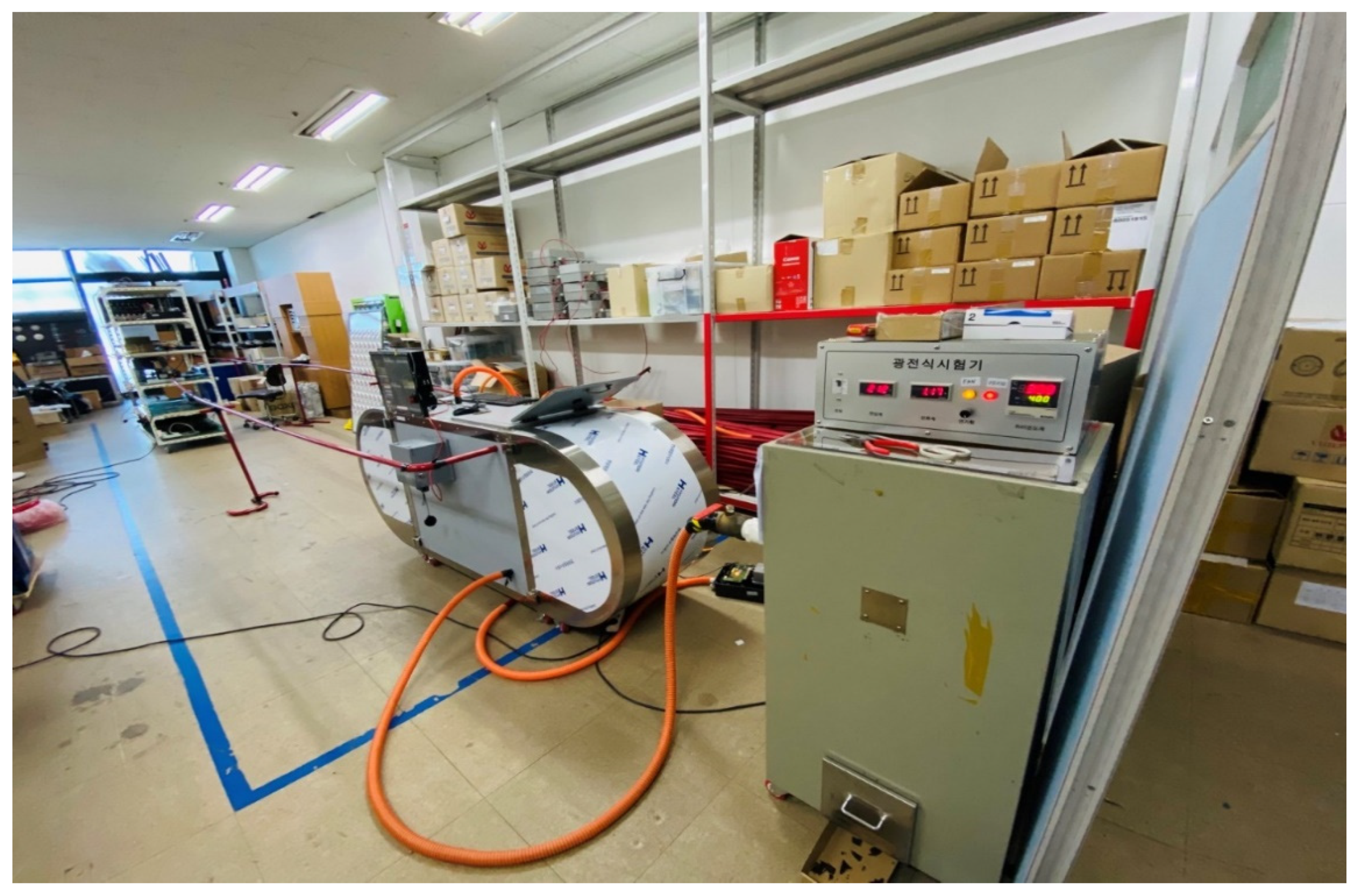
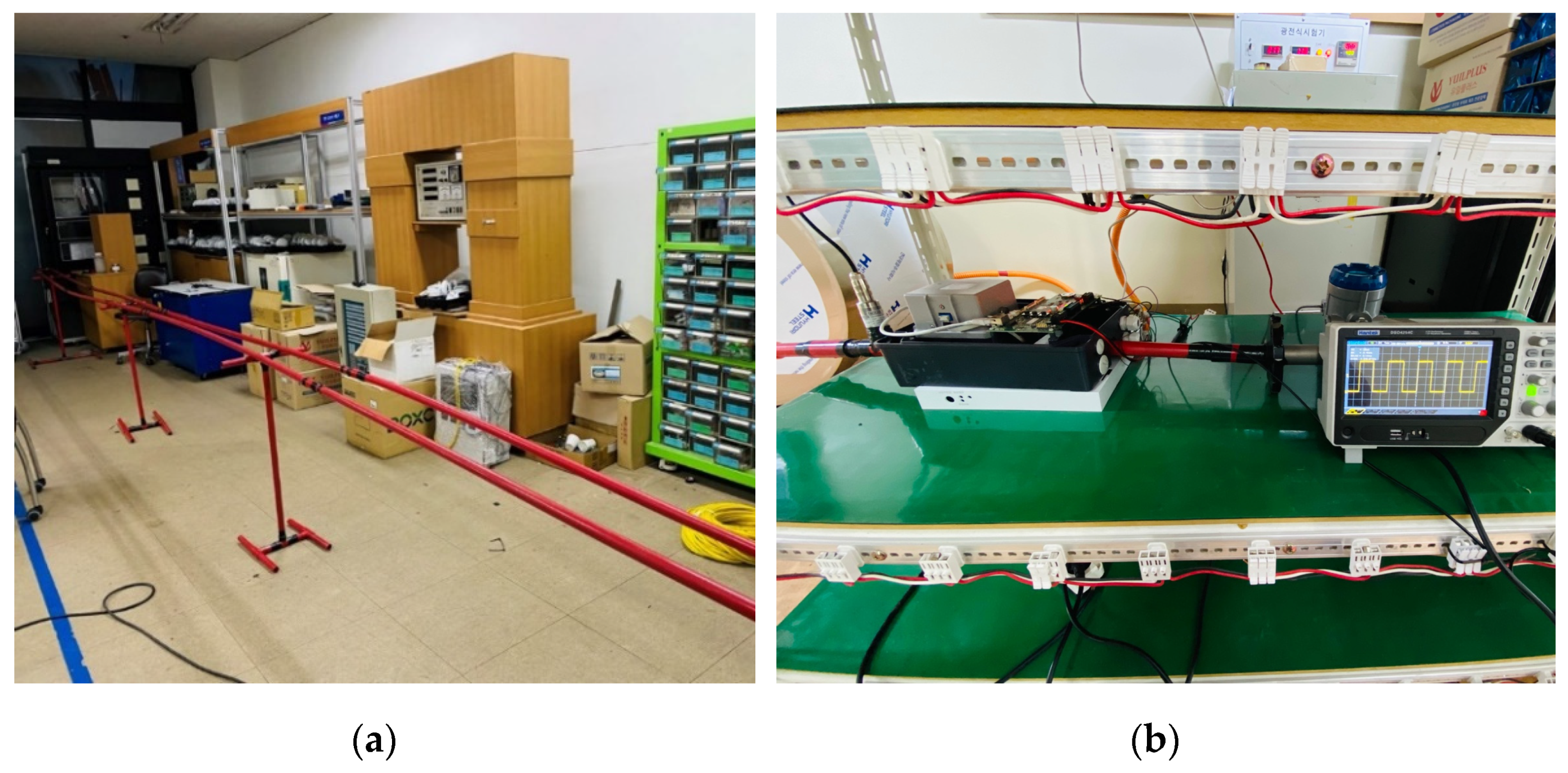
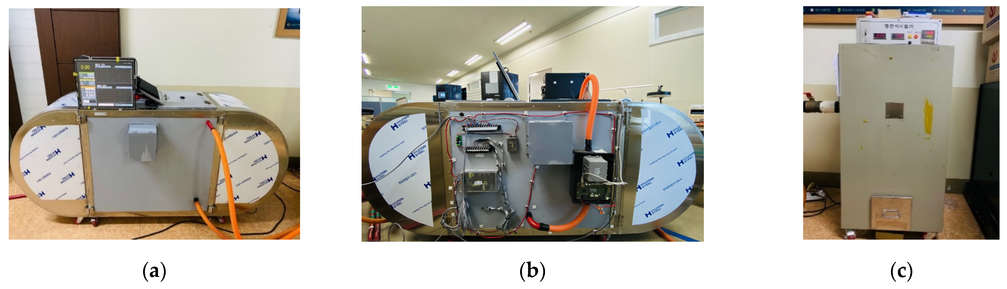
3.2. Experimental Study

In this study, the effect of the pipe hole network on obscuration in the aspirating smoke detection system was investigated. For that purpose, the smoke flow through the pipe was considered. The pipe length was 20 m, and ten holes with a diameter of 5 mm were drilled in the pipe. The distance between every hole was 2 m. The ASD system with a smokebox and pipe is shown in Figure 2. The schematic diagram of the experiment was represented in Figure 3 and specifications of the experimental apparatus were represented in

Table A1. Specification of experimental apparatus.

Technical Data	Specification	ASD 532
Supply voltage range	EN 54	14.0–30 VDC
	FM/UL	16.4–27 VDC
Power consumption	Typical for 24 VDC	115 mA
Sampling tubes	Quantity	1
Alarm sensitivity	Alarm	0.02–10%/m
Monitoring area	Max. area	1280 m2
System limits without conformity to standards	Max. overall length of all sampling tubes	120 m
Fan/sampling system	Suction pressure Service life (MTTF) Noise level (1 m distance)	>100 Pa >8000 h (at 40 °C) 25 dB(A)
Airflow monitoring	As per EN 54-20	1 air flow sensor
Flow meter	Output: DC 4–20 mA, Range: 0~30 Nm3/h, Accuracy: ±0.5% Model: KSMG-8000
Pressure sensor	Range: 0–25 mbar, Accuracy: 0.2% Model: CPH6300
Oscilloscope	Output Voltage: About 2 Vpp into ≥ 1 MΩ, Band: 250 Mhz, Frequency Resolution: 0.1% Model: DSO4254C
Light meter	Digital Output: USB, Range: 0.01 to 299,900 lx; Accuracy: ±2% ±1 digit of displayed value Model: Illuminace Meter T-10A

.

The general operating principle of the ASD is shown in Figure 4. In the pipe hole network, the fan generates a vacuum which results in fresh air reaching the detector housing through the pipe holes. The smoke sensor is supplied with new airflow from the monitoring area. As the obscuration in ASD exceeds the setup value, the ASD triggers an alarm. The specification of the ASD system can be referred at [31].

In this system, two pieces of aspirating smoke detection equipment were used. ASD 1 was connected directly to the straight pipe to measure the obscuration in the pipe, and ASD 2 was connected to the smokebox for monitoring the smokebox obscuration to maintain obscuration as constant. In the experiment, the smokebox obscuration was 5%/m, 10%/m, and 15%/m. For each respective smokebox obscuration, the location of the smokebox was changed from the first hole to the last hole to find the relation between fire source location and obscuration at ASD 1.

In order to measure the obscuration in the aspirating smoke detection system, the pipe which had the hole was put into the smokebox, and the smoke moved from the smokebox through a pipe hole to ASD 1. At ASD 1, the obscuration was recorded and displayed on computer 1. The experiment was shown in Figure A1, Figure A2 and Figure A3.

Firstly, the fire was generated in the smokebox. After that, the obscuration in the smokebox was set up as 5%/m (controlled by ASD 2). Then, the smoke moved from the smokebox to ASD 1, so the value of obscuration at ASD 1 was recorded. The experiment at hole 1 was performed three times to obtain the accuracy value. After measuring with 5%/m obscuration in the smokebox, the obscuration in the smokebox was changed from 5% to 10%/m, and 15%/m, respectively. The data at ASD 1 were re-recorded.

Similarly, the location of the smokebox was changed from the first hole to the last hole. At every hole, the obscuration in the smokebox was set up as 5%, 10% and 15%/m, respectively.

4. Results and Discussion

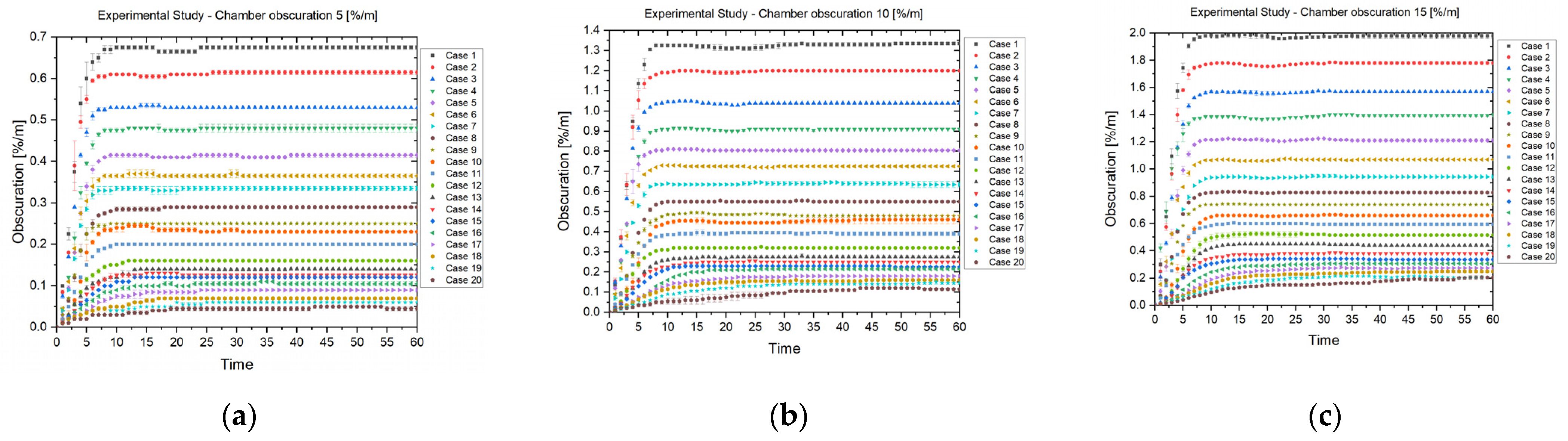
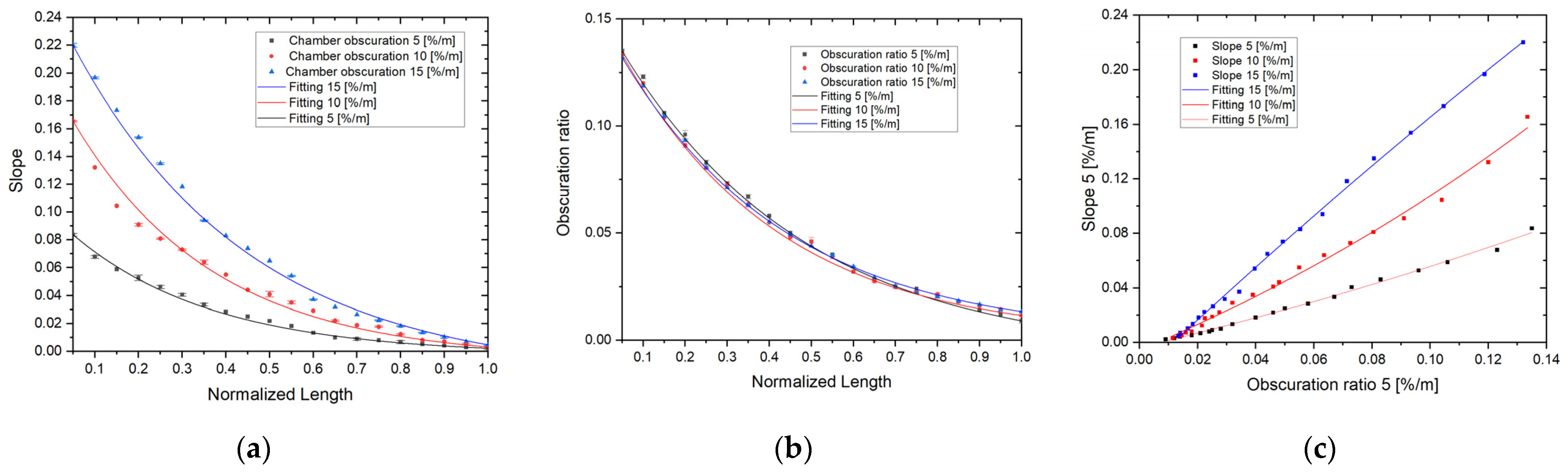
4.1. ASD System with One Branch Pipe with Ten Holes

The obscuration data in the ASD system is shown in Figure 5. From case 1 to case 10, the location of the smokebox is from hole 1 to hole 10, respectively. When the smoke went through the pipe to ASD 1, the obscuration was totally different from hole 1 to hole 10. The pressure at ASD 1 for one branch pipe with ten holes in the experiment was −90 ± 2 Pa.

In Figure 5a, the obscuration in the smokebox is shown to be 5%/m. Obscuration was measured at ASD. Firstly, when the smokebox was located at hole 1, the obscuration at ASD 1 was around 0.95%/m, and the obscuration at ASD 1 when the smokebox located at hole 10 was 0.37%. The reason for this is that the flow rate through the hole was not equal. In this study, all holes had the same size as 5 mm, so that at the hole, which is nearest to the ASD, the pressure difference between inside and outside of the hole is largest, so the fluid that goes through that hole has the largest flow rate. This means that the flow rate of smoke from the smokebox to ASD 1 was also larger. So, the obscuration of hole 1 was the largest (0.95%/m). In addition, when the fluid moved through the pipe hole, a pressure drop also occurred. On the other hand, when the smokebox was connected with hole 10, the flow rate from the smokebox to the ASD was the smallest. Thus, the obscuration at ASD 1 was the smallest too (0.37%/m).

Similarly, when the obscuration in the smokebox was changed from 5 to 10, and 15%/m, the value of obscuration was as shown in Figure 5b,c. It had the same trend as shown previously in Figure 5a. The detail obscuration at ASD when the chamber obscuration is 5, 10, 15%/m is shown in

Table 3. The obscuration at ASD 1 when chamber obscuration is 5%/m.

	Hole 1	Hole 2	Hole 3	Hole 4	Hole 5	Hole 6	Hole 7	Hole 8	Hole 9	Hole 10
Obscuration (%/m)	0.95	0.85	0.74	0.67	0.6	0.55	0.45	0.42	0.4	0.37

,

Table 4. The obscuration at ASD 1 when chamber obscuration is 10%/m.

	Hole 1	Hole 2	Hole 3	Hole 4	Hole 5	Hole 6	Hole 7	Hole 8	Hole 9	Hole 10
Obscuration (%/m)	1.74	1.54	1.38	1.24	1.1	0.98	0.91	0.85	0.8	0.76

and

Table 5. The obscuration at ASD 1 when chamber obscuration is 15%/m.

	Hole 1	Hole 2	Hole 3	Hole 4	Hole 5	Hole 6	Hole 7	Hole 8	Hole 9	Hole 10
Obscuration (%/m)	2.52	2.23	2.02	1.79	1.59	1.48	1.36	1.2	1.17	1.07

.

Based on the Pipe Hole Network Program, the obscuration in a pipe with 10 sampling holes was considered. The locations of holes 1 to hole 10 were 2, 4, 6, 8, 10, 12, 14, 16, 18, and 20 m, respectively. Figure 6 shows the numerical and experimental obscuration values through the pipe hole for different chamber obscuration values.

In order to predict the fire source location by using ASD, the slope and obscuration ratio of ASD were investigated:

$$Obscuration ratio=\frac{ASD Obscuration}{Chamber obscuration}$$

(22)

The slope and obscuration ratio at ASD when the chamber obscuration is 5, 10, 15%/m is shown below in

Table 6. The slope and obscuration ratio at ASD 1 when chamber obscuration is 5%/m.

Hole	Slope	ASD Obscuration (%/m)	Chamber Obscuration (%/m)	Obscuration Ratio (%/m)
1	0.10556	0.9533	5	0.1907
2	0.09407	0.84667	5	0.1693
3	0.08222	0.7400	5	0.148
4	0.07444	0.66667	5	0.1334
5	0.06	0.60333	5	0.1207
6	0.0490	0.55	5	0.11
7	0.03359	0.44667	5	0.089
8	0.025625	0.42333	5	0.084
9	0.019048	0.4033	5	0.081
10	0.00982	0.3733	5	0.0747

,

Table 7. The slope and obscuration ratio at ASD 1 when chamber obscuration is 10%/m.

Hole	Slope	ASD Obscuration (%/m)	Chamber Obscuration (%/m)	Obscuration Ratio (%/m)
1	0.1952	1.74	10	0.174
2	0.1707	1.54	10	0.154
3	0.1387	1.38	10	0.138
4	0.1124	1.24	10	0.124
5	0.0994	1.1	10	0.11
6	0.0754	0.983	10	0.098
7	0.0645	0.91	10	0.091
8	0.0444	0.853	10	0.085
9	0.0315	0.8	10	0.08
10	0.0241	0.76	10	0.076

and

Table 8. The slope and obscuration ratio at ASD 1 when chamber obscuration is 15%/m.

Hole	Slope	ASD Obscuration (%/m)	Chamber Obscuration (%/m)	Obscuration Ratio (%/m)
1	0.2796	2.523	15	0.168
2	0.224	2.23	15	0.149
3	0.1821	2.02	15	0.135
4	0.1519	1.787	15	0.119
5	0.1233	1.593	15	0.1061
6	0.0976	1.483	15	0.098
7	0.0845	1.363	15	0.0908
8	0.0571	1.203	15	0.0802
9	0.0426	1.17	15	0.078
10	0.0321	1.073	15	0.0715

.

In Figure 7a, the correlation between slope and normalized length was investigated. In that, the normalized length is the location of the hole over the total length. When the smokebox is located at the hole near the ASD, the slope is largest. On the other hand, when the smokebox is located at the hole which is far away from the ASD, the slope is smallest. Similarly, the obscuration ratio in the ASD had the same trend as the slope in Figure 7b, the obscuration ratio is largest at the hole which is located nearby to the ASD. Besides, the correlation between the slope and obscuration ratio is shown in Figure 7c.

The fitting correlation between normalized length and slope in Figure 7a were derived as the following Equations (23)–(25) for 5%/m, 10%/m, and 15%/m chamber obscuration cases, respectively.

$$S=0.1425e^{(-\overline{L}/0.4305)}+0.002$$

(23)

$$\mathrm{S}=0.2515e^{(-\overline{L}/0.4505)}+0.001$$

(24)

$$S=0.36801e^{(-\overline{L}/0.54565)}-0.02676$$

(25)

where S is the slope, $\overline{L}$ is normalized length.

Similarly, the fitting correlation between normalized length and obscuration ratio in Figure 7b was derived as the following Equations (26)–(28) for chamber obscuration 5%/m, 10%/m, 15%/m.

$$R=0{.17608\mathrm{e}}^{(-\overline{L}/0.59593)}+0.04178$$

(26)

$$R=0{.145438\mathrm{e}}^{(-\overline{L}/0.54049)}+0.05314$$

(27)

$$R=0{.14623\mathrm{e}}^{(-\overline{L}/0.58791)}-0.04487$$

(28)

where R is obscuration ratio, $\overline{L}$ is normalized length.

From Figure 7a,b, the correlation between slope and obscuration ratio were shown as Figure 7c, and correlation equations were derived as Equations (29)–(31):

$$S=-0{.2866}^{(-R/0.10141)}+0.14885$$

(29)

$$S=-0{.6143\mathrm{e}}^{(-R/0.18062)}+0.42904$$

(30)

$$S=2{.19466\mathrm{e}}^{(-R/-0.98412)}-2.32702$$

(31)

From the Equations (23)–(25), the fire source location can be determined as the following equations:

$$\overline{L}=-0.4305\times \ln \left(\frac{S-0.002}{0.1425}\right)$$

(32)

$$\overline{L}=-0.4505\times \ln \left(\frac{S-0.001}{0.2515}\right)$$

(33)

$$\overline{L}=-0.54565\times \ln \left(\frac{S+0.02676}{0.36801}\right)$$

(34)

Based on Equations (32)–(34), the fire source location can be determined with chamber obscuration of 5, 10, 15%/m, respectively.

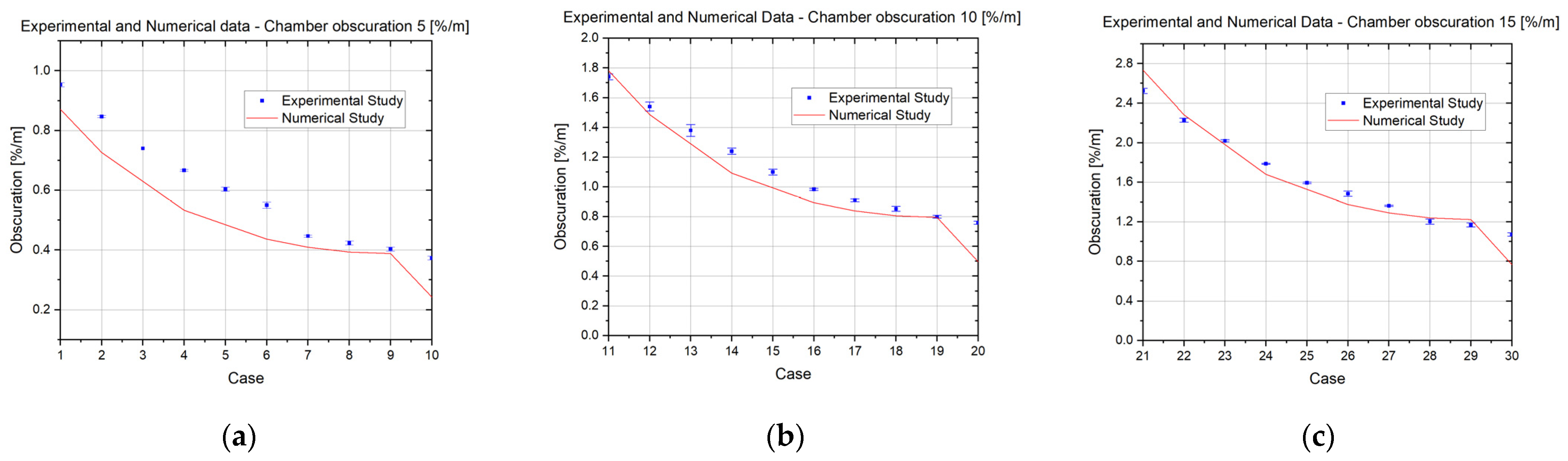
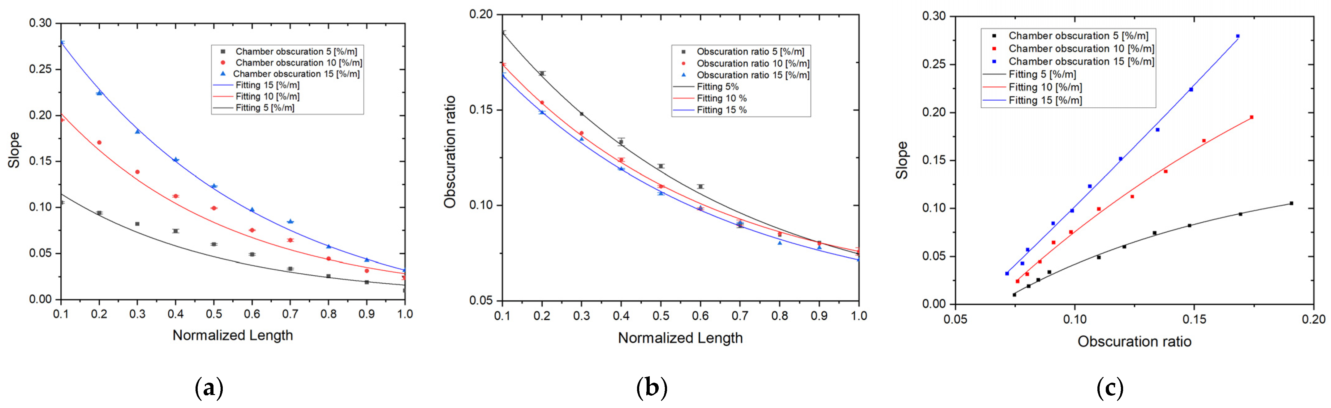
4.2. ASD System with One Branch Pipe with Twenty Holes

The obscuration in the ASD system is shown in Figure 8. From case 1 to case 20, the location of the smokebox is from hole 1 to hole 20, respectively. When the smoke went through the pipe to ASD 1, the obscuration was different from hole 1 to hole 20. The pressure at ASD 1 for one branch pipe with twenty holes in the experiment was −69 ± 1.5 Pa.

In Figure 8a, the obscuration in the smokebox is shown to be 5%/m. Obscuration was measured at ASD. Firstly, when the smokebox was located at hole 1, the obscuration at ASD 1 was around 0.68%/m, and the obscuration at ASD 1 when the smokebox located at hole 20 was 0.045%. It means, the further away from the location it is, the lower the obscuration is.

The obscuration data was shown in Figure 8b,c when the smoke chamber was set at 10%/m and 15%/m, respectively.

The slope and obscuration ratio of ASD were also investigated. The value of these parameters was shown in Figure 9.

Similarly, the slope and obscuration ratio were investigated to predict the fire source location. In Figure 9a, the relation between slope and normalized length was performed. When the smokebox is located at the hole near the ASD, the slope is largest. On the other hand, when the smokebox is located at the hole which is far away from the ASD, the slope is smallest. Moreover, the obscuration ratio in the ASD had the same trend as the slope in Figure 9b, the obscuration ratio is largest at which hole is located nearby the ASD. It had the same trend when the pipe had ten holes in Section 4.1.

The fitting correlation between normalized length and slope in Figure 9a were derived as the following Equations (35)–(37) for the chamber obscuration 5%/m, 10%/m, and 15%/m, respectively.

$$S=0.10045{\mathrm{e}}^{(-\overline{L} /0.3217)}-0.00224$$

(35)

$$S=0.20022{\mathrm{e}}^{(-\overline{L} /0.31965)}-0.0056$$

(36)

$$S=0.2692{\mathrm{e}}^{(-\overline{L} /0.4029)}-0.01778$$

(37)

where S is the slope, $\overline{L}$ is normalized length.

Similarly, the fitting correlation between the normalized length and obscuration ratio in Figure 9b were derived as the following Equations (38)–(40) for chamber obscuration 5%/m, 10%/m, 15%/m.

$$R=0.15971{\mathrm{e}}^{(-\overline{L} /0.44202)}-0.00763$$

(38)

$$R=0.15146{\mathrm{e}}^{(-\overline{L} /0.37618)}+0.000887$$

(39)

$$R=0.14815{\mathrm{e}}^{(-\overline{L} /0.39748)}+0.00136$$

(40)

where R is obscuration ratio, $\overline{L}$ is normalized length.

From the Equations (35)–(37), the fire source location can be determined as the following equations with chamber obscurations of 5%, 10%, 15%/m, respectively.

$$\overline{L}=-0.3217\times \ln \left(\frac{S+0.00224}{0.10045}\right)$$

(41)

$$\overline{L}=-0.31965\times \ln \left(\frac{S+0.0056}{0.20022}\right)$$

(42)

$$\overline{L}=-0.4029\times \ln \left(\frac{S+0.01778}{0.2692}\right)$$

(43)

When the fire occurs, the obscuration can be obtained at the ASD. From the obscuration data, the slope (S) of obscuration can be calculated. By applying Equations (41)–(43), the three predicted fire source location can be achieved. Using three predicted fire source locations to apply in Equations (38)–(40), the three-obscuration ratio can be obtained. Comparing these equation obscuration ratios with the experimental obscuration ratio, the exact obscuration ratio can be obtained and the exact fire source location can be derived.

Based on Section 4.1 and Section 4.2, the results show that the obscuration in the ASD system is not equal when the location of the smokebox is changed. When a fire occurs at the nearest hole, the obscuration is the largest.

By changing the number of the hole in the pipe, the obscuration in aspirating smoke detection is changed. When increasing the number of holes on the pipe, the obscuration at the ASD decreases.

The obscuration value at ASD 1 has the same trend for different obscuration values in the smokebox. This shows that the highest obscuration value occurs at the nearest holes, and the lowest obscuration value occurs at the farthest away hole.

The numerical study showed the same trend as an experimental study. The further away the location of the smokebox is, the lower the obscuration is. This means that numerical studies can be used to predict obscuration in further research.

5. Conclusions

In this study, the effect of the pipe hole on the obscuration in the ASD system to predict the fire source location was investigated by numerical and experimental studies.

The correlation between slope, obscuration ratio and the fire source location can be represented by length Equations (32)–(34) and (41)–(43) to determine the fire source location in the ASD system with different cases. When the given obscuration smoke moves through any hole, the smoke obscuration at the ASD was obtained, so the obscuration ratio and slope were derived. By applying those equations, the normalized length can be calculated, so the fire source location can be predicted.

In this research, the short pipe, as well as three given chamber obscurations, 5%, 10%, 15%/m, were investigated as a first approach to predict the fire source location by the ASD. However, in a real fire, the smoke obscuration could vary with time. So, in further work, the various smoke obscurations will be investigated and machine learning methods could be applied to predict the fire source location in the real fire phenomena.

References

1. Cheng, L.; Zhou, H.; Yang, H. The Simulation of the Sampling Pipes and Sampling Holes Network with an Aspirating Smoke Detector. In Proceedings of the JFPS International Symposium on Fluid Power, Tsukuba, Japan, 7–10 November 2005; The Japan Fluid Power System Society: Tokyo, Japan, 2005; Volume 2005, pp. 386–390. [Google Scholar]
2. Carello, M.; Ivanov, A.; Mazza, L. Pressure drop in pipe lines for compressed air: Comparison between experimental and theoretical analysis. WIT Trans. Eng. Sci. 1970, 18, 10. [Google Scholar]
3. Essienubong, I.A.; Ejiroghene, K.O. Pressure Losses Analysis in Air Duct Flow Using Computational Fluid Dynamics (CFD). Int. Acad. J. Sci. Eng. 2016, 3, 55–70. [Google Scholar]
4. Gajbhiye, B.; Kulkarni, H.A.; Tiwari, S.S.; Mathpati, C.S. Teaching turbulent flow through pipe fittings using computational fluid dynamics approach. Eng. Rep. 2020, 2, e12093. [Google Scholar] [CrossRef] [Green Version]
5. Perumal, K.; Rajamohan, G. CFD modeling for the estimation of pressure loss coefficients of pipe fittings: An undergraduate project. Comput. Appl. Eng. Educ. 2016, 24, 180–185. [Google Scholar] [CrossRef]
6. Singh, R.K. A Study of Air Flow in a Network of Pipes Used in Aspirated Smoke Detectors. Ph.D. Thesis, Victoria University, Melbourne, Australia, 2009. [Google Scholar]
7. Gai, Y.; Cai, M.; Shi, Y. Analytical and experimental study on complex compressed air pipe network. Chin. J. Mech. Eng. 2015, 28, 1023–1029. [Google Scholar] [CrossRef]
8. Huang, Y.; Wang, E.; Bie, Y. Simulation investigation on the smoke spread process in the large-space building with various height. Case Stud. Therm. Eng. 2020, 18, 100594. [Google Scholar] [CrossRef]
9. Huang, Y.; Chen, X.; Zhang, C. Numerical simulation of the variation of obscuration ratio at the fire early phase with various soot yield rate. Case Stud. Therm. Eng. 2020, 18, 100572. [Google Scholar] [CrossRef]
10. Zhenna, Z.; Qin, Z.; Hongbing, C.; Suilin, W.; Hongwen, L. Performance study on fire alarm system in large space buildings. In Recent Advances in Computer Science and Information Engineering; Springer: Berlin/Heidelberg, Germany, 2012; pp. 69–73. [Google Scholar]
11. Krope, J.; Dobersek, D.; Goricanec, D. Flow pressure analysis of pipe networks with linear theory method. In Proceedings of the 2006 WSEAS/IASME International Conference on Fluid Mechanics, Miami, FL, USA, 18–20 January 2006. [Google Scholar]
12. Qian, Y.; Zhu, D.Z.; Edwini-Bonsu, S. Air flow modeling in a prototype sanitary sewer system. J. Environ. Eng. 2018, 144, 04018008. [Google Scholar] [CrossRef]
13. Quraishi, M.S. Prediction of fan assisted flow in a duct/pipe network. In Proceedings of the 1996 CNA/CNS Conference, Fredericton, NB, Canada, 9–12 June 1996. [Google Scholar]
14. Brkić, D.; Praks, P. An efficient iterative method for looped pipe network hydraulics free of flow-corrections. Fluids 2019, 4, 73. [Google Scholar] [CrossRef] [Green Version]
15. Lang, S. Variable Air Speed Aspirating Smoke Detector. U.S. Patent 8,098,166, 17 January 2012. [Google Scholar]
16. Nagy, T.; Jílek, A.; Pečínka, J. Air flow rate measurement with various differential pressure methods. In Proceedings of the 2017 International Conference on Military Technologies (ICMT), Brno, Czech Republic, 31 May–2 June 2017; IEEE: Piscataway, NJ, USA, 2017; pp. 535–541. [Google Scholar]
17. Anantharaman, V.; Waterson, N.; Nakiboglu, G.; Persin, M.; van Oudheusden, B. Experimental investigation of turbulent flow through single-hole orifice placed in a pipe by means of time-resolved Particle Image Velocimetry and unsteady pressure measurements. In Proceedings of the 11th International Conference on Flow-Induced Vibrations, Den Haag, The Netherlands, 4–6 July 2016. [Google Scholar]
18. Grant, G.; Drysdale, D. Numerical modelling of early flame spread in warehouse fires. Fire Saf. J. 1995, 24, 247–278. [Google Scholar] [CrossRef]
19. Lönnermark, A.; Ingason, H. Fire Spread in Large Industrial Premises and Warehouse; SP Swedish National Testing and Research Institute: Borås, Sweden, 2005. [Google Scholar]
20. Muckett, M.; Furness, A. Introduction to Fire Safety Management; Routledge: London, UK, 2007. [Google Scholar]
21. Liu, S.; Luo, X.; Yao, W.; Chen, C.; Kun, Y.; Yi, M.; Hu, H.; Zhang, Y. Aspirating fire detection system with high sensitivity and multi-parameter. In Proceedings of the 2014 International Conference on Information Science, Electronics and Electrical Engineering, Sapporo, Japan, 26–28 April 2014; IEEE: Piscataway, NJ, USA, 2014. [Google Scholar]
22. Shaltout, R.E.; Ismail, M.A. Simulation of Fire Dynamics and Firefighting System for a Full-Scale Passenger Rolling Stock. In Sustainable Rail Transport; Springer: Cham, Switzerland, 2020; pp. 209–228. [Google Scholar]
23. Johnson, P.; Beyler, C.; Croce, P.; Dubay, C.; McNamee, M. Very Early Smoke Detection Apparatus (VESDA), David Packham, John Petersen, Martin Cole: 2017 DiNenno Prize. Fire Sci. Rev. 2017, 6, 1–12. [Google Scholar] [CrossRef] [Green Version]
24. Zhang, Z.N.; Chen, H.B. Simulation Study on the Aspirating Smoke Detection System in Large Space Buildings. In Advanced Materials Research; Trans Tech Publications: Baech, Switzerland, 2011; Volume 255, pp. 1404–1408. [Google Scholar]
25. Brown, G.O. The history of the Darcy-Weisbach equation for pipe flow resistance. In Proceedings of the Environmental and Water Resources History Sessions at ASCE Civil Engineering Conference and Exposition, Washington, DC, USA, 3–7 November 2002; ASCE: Reston, VA, USA, 2003; pp. 34–43. [Google Scholar]
26. Cole, M. Disturbance of Flow Regimes by Jet Induction. Ph.D. Thesis, Victoria University of Technology, Melbourne, Australia, 1999. [Google Scholar]
27. Munson, B.R.; Young, D.F.; Okiishi, T.H. Fundamentals of Fluid Mechanics; John Wiley & Sons: Hoboken, NJ, USA, 1998; pp. 199–200. [Google Scholar]
28. McDermott, R.; McGrattan, K.; Hostikka, S. Fire dynamics simulator (version 5) technical reference guide. NIST Spec. Publ. 2008, 1018, 5. [Google Scholar]
29. Fabian, T.Z.; Gandhi, P.D. Smoke Characterization Project; Fire Protection Research Foundation/Underwriters Laboratories, Incorporated: Quincy, MA, USA, 2007. [Google Scholar]
30. Miller, J.H.T., IV. Analyzing Photo-Electric Smoke Detector Response Based on Aspirated Smoke Detector Obscuration; University of Maryland: College Park, MD, USA, 2010. [Google Scholar]
31. Securition: SecuriSmoke ASD Aspirating Smoke Detectors the Complete Model Range for Any Application. Available online: https://www.securiton.com/products-services/smoke-detection-systems/securismoke-asd (accessed on 26 January 2022).
Figure 1. The sketch of the pipe hole.
Applsci 12 02801 g001
Figure 2. The aspiration smoke detection system with the smokebox and straight pipe.
Applsci 12 02801 g002
Figure 3. Schematic diagram of experiment used to determine the obscuration in aspirating smoke detection system.
Applsci 12 02801 g003
Figure 4. General operating principle of ASD.
Applsci 12 02801 g004
Figure 5. The obscuration at ASD (a) The obscuration at ASD when chamber obscuration was 5%/m (b) The obscuration at ASD when chamber obscuration was 10%/m (c) When chamber obscuration was 15%/m.
Applsci 12 02801 g005
Figure 6. The comparison of obscuration between the numerical and experimental studies (a) When the chamber obscuration is 5%/m (b) When the chamber obscuration is 10% (c) When chamber obscuration is 15%/m.
Applsci 12 02801 g006
Figure 7. (a) The slope and normalized length correlation; (b) The obscuration ratio and normalized length correlation; (c) The slope and obscuration ratio correlation.
Applsci 12 02801 g007
Figure 8. The obscuration at ASD (a) When chamber obscuration was 5%/m (b) When chamber obscuration was 10%/m (c) When chamber obscuration was 15%/m.
Applsci 12 02801 g008
Figure 9. (a) The slope and normalized length correlation; (b) the obscuration ratio and normalized length correlation; (c) the slope and obscuration ratio correlation.
Applsci 12 02801 g009