1. Introduction
Continuous measurements at geomagnetic observatories are a very important source for understanding short-term and long-term changes in the geomagnetic field, both due to variations in the Earth’s interior and the near-Earth environment. Across the globe, 153 INTERMAGNET observatories are providing uninterrupted measurements of vector and scalar components of the Earth’s magnetic field, and the Hyderabad Magnetic Observatory (HYB) is one among them. Further advances in studies of the internal and external field in combination with data from satellites requires much higher accuracies and resolution of data. Monitoring the geomagnetic field is of crucial importance in today’s technology-dependent world (e.g., for satellite health and telecommunication systems).
Disturbances in the magnetic measurements from electrical railways have previously been studied; theoretical calculations of the magnetic field values generated by DC railway cars have been developed [
1,
2]. Ref. [
3] studied disturbances in geomagnetic measurements at BJI Observatory, caused by direct current (DC) railway systems, and proposed a noise reduction method based on the adaptive Kalman filter. Disturbances from power lines in the magnetic data have been identified and quantified by [
4,
5,
6]. Ref. [
7] reported and rectified different sources of anthropogenic noise due to heavy vehicle movements, power fluctuation problems, etc. Ref. [
8] reported perturbances in the Easter Island observatory, produced by trucks’ movements at a stone quarry located near to the observatory campus, and also due to the movement of airplanes 100 m away from the measurement site. Ref. [
9] performed a detailed analysis on the factors that affect total field measurements.
To meet the international standards, observatory staff make meticulous efforts to deliver a good quality geomagnetic time series data by using algorithms to detect and remove the noise in HYB Observatory data caused by the metro line, based on its structural stability. The algorithm works as follows: when a change in dZ between neighboring measurements (in absolute value), exceeding a given threshold, is found, three subsequent measurements are discarded. It is clear that this algorithm creates the following risks: (a) natural signals with sharp edges, for example, during magnetic disturbances, may be discarded; (b) noise may be incompletely removed if its duration is long; (c) noise can be missed if, due to a small shift, its leading edge takes two samples. However, to calculate the minute values of magnetic field variations, this may be enough [
7]. Representing the natural field variations is becoming a challenging task, due to increased construction, public transportation and development activities around the magnetic observatories, which has become a source of degradation of magnetic data quality. The parameters that affect the data quality depend on the instrument characteristics, data resolution, expertise of the observer and characteristics of the geomagnetic field, defined by the specific location of a magnetic observatory. Such parameters could be natural (temperature, humidity, groundwater circulation, telluric currents, frequency of lightning, magnetic gradient, etc.) or man-made (AC and DC sources in the vicinity of the sensor, sensor alignment, time stamping, etc.). Due to the increase in urban expansion, as well as the infrastructural facilities in cities, producing good quality and highly accurate geomagnetic measurements by cleaning the artificial noise is increasingly difficult, even though the observatories were originally built in magnetically quiet locations. In this context, to maintain good data quality, it is necessary to understand and assess the factors associated with changing environmental day-to-day conditions that influence data quality, so as to improve the data acquisition and processing procedure accordingly.
During the COVID-19 pandemic situation, the INTERMAGNET Hyderabad Observatory has committed to continue its operations in recording the Earth’s magnetic field without any interruption even with very limited staff during the nationwide lockdown in India (from 24 March to 17 May 2020). An attempt is made to identify and characterize the anthropogenic noise due to metro rail services and vehicular traffic on the 1s data quality of vector and scalar magnetic measurements at HYB.
2. Data and Results
In order to achieve the aim of the study, we studied and analyzed the 1 Hz vector variation HDZ data acquired from a tri-axial fluxgate magnetometer and the 1 Hz scalar variation (F) data acquired from a GSM90-F1 magnetometer for 50 days before and 50 days during lockdown (1 February to 10 May 2020). Quiet days were chosen in March (before lockdown) and compared with April 2020 (during lockdown) for the analysis. Further, we used the vector and scalar data from the Choutuppal (CPL) Magnetic Observatory of this institute, 65 km away from HYB, for comparison. The CPL Observatory is located in a 100 acre campus, and is relatively far from sources of anthropogenic and cultural noises.
International quiet (IQ) days vary from the highest to the lowest order of quietness and disturbance, respectively [
10]. This classification leads to the study of the different physical processes in the ionosphere and magnetosphere, which cause variations in the geomagnetic field. The K-index is defined as a quasi-logarithmic measure, ranging in steps of one, from zero to nine, of the range of geomagnetic disturbance at a geomagnetic observatory in a three-hourly UT interval (00–03, 03–06, …, 21–24) [
1]. The K-sum is the sum of all 3 h interval K-index values of one day. The IQ days of March 2020 were 14, 11, 5, 10 and 7 prior to lockdown (K-sum was 4, 4, 8, 7 and 6, respectively), and in April 2020, they were 30, 29, 06, 23 and 17 during lockdown (K-sum was 1, 3, 3, 5 and 5, respectively). The diurnal geomagnetic field variations in H, D, Z and F (for quiet days, 11 March (DoY 71) and 6 April 2020 (DoY 97)) are shown in
Figure 1 (top and bottom panel).
In
Figure 1, the top panel indicates the raw variations in the geomagnetic field at HYB (vector and scalar) on quiet days before lockdown, i.e., 11 March 2020, and the bottom panel indicates the data during lockdown, i.e., 6 April 2020. Blue and red colors indicate the H and D components. Visually, it appears that there is no significant change in data quality before and during lockdown. The green and black lines indicate the Z and F components’ variation data. Comparing the Z and F components before and during lockdown periods shows a visibly reduced frequency of noise peaks during lockdown. We also noticed spikes with an amplitude of around 7 nT in the Z and F components in the period before lockdown, whereas an amplitude of around 4 nT is observed during the lockdown period.
The maximum amplitude of first difference is ±0.2 nT in the H and D components both before and during lockdown, while it is ±4 nT in Z before lockdown, which is reduced to ±3 nT during lockdown (
Figure 2, top panel in green). The spikes with an amplitude between 3 and 4 nT are reduced by eight times in the lockdown period, when compared to before lockdown. Similarly, the amplitude of spikes between 1 and 3 nT in the lockdown period are reduced by half when compared to before lockdown. The maximum amplitude of first difference of the F component is noted as ±2 nT, both before and during lockdown. The range of first difference values in each component is independent of the magnetic activity levels. Additional case studies for before and during lockdown are provided in
Figures S1 and S2 in the Supplementary Information.
We also tried to assess whether the reduction in noise during lockdown affected the quality of absolute measurements. These absolute observations are performed manually on a weekly basis using a DI single-axis fluxgate magnetometer, producing spot values of D and I specific to a time at that location. Simultaneous scalar-F measurements are also carried out during the period of D/I observations, from which the absolute values of the H, D and Z components are derived.
Figure 3 shows the absolute values of D, I and F from February 2020 to May 2020. The red color depicts the spot values from before lockdown and the green color depicts those during lockdown. Some variations in spot values can be ascribed to the different times of day at which measurements were performed. Overall, the I and F spot values are more consistent compared to D. Scatter between the absolute measurements of D, I and F carried out on the same day ranges from 0.05 to 0.5 min, 0.03 to 0.1 min and 0.6 to 3.6 nT, respectively, before lockdown, and 0.07 to 0.6 min, 0.02 to 0.5 min and 0.6 to 2.1 nT during lockdown.
These absolute measurements were used to calculate the baselines of H, D and Z, which are necessary to prepare definitive data of the geomagnetic field components. Having assessed the amplitudes of noise in the variation data and absolute measurements of D and I, we checked the effect on the calculated baselines (only for 86 days, including the lockdown period). These baselines were processed by only considering those spot values of absolute and variation data, which are consistent and devoid of noise, and excluding data points that have high noise levels during the period of observation. In
Figure 4, the left side (red) portion indicates the baselines of H, D and Z before lockdown and the right side (green) is during the lockdown period. Over the observation period (45 days), the baseline variation range was about 0.6 nT, 0.06 min and 0.4 nT in the H, D and Z components, respectively, before lockdown. During the period of lockdown (42 days), the corresponding values changed slightly to 0.4 nT, 0.05 min and 0.8 nT, respectively. The standard deviations of measurements from the calculated baselines reduced by 25–50% in the different components during the lockdown period, compared to normal traffic conditions, as shown in
Table 1. The averages of the differences in amplitudes between consecutive values of calculated baselines for each day of absolute measurement were 0.29 nT, 0.05 min and 0.13 nT for H
B, D
B and Z
B before lockdown, and 0.24, 0.03 and 0.17 during lockdown, showing that the baselines were undisturbed by the vehicular noise, as shown in
Table 2.
3. Noise Characteristics
We calculated the noise spectra in the HYB data and identified the outliers, which will provide information about the deviation of these points from the mean value. With the available information from the outliers, we designed a zero-phase forward low-pass Butterworth filter of order six, with a cut-off frequency 0.01 Hz, to eliminate the noise in the Z and F components of the HYB raw data.
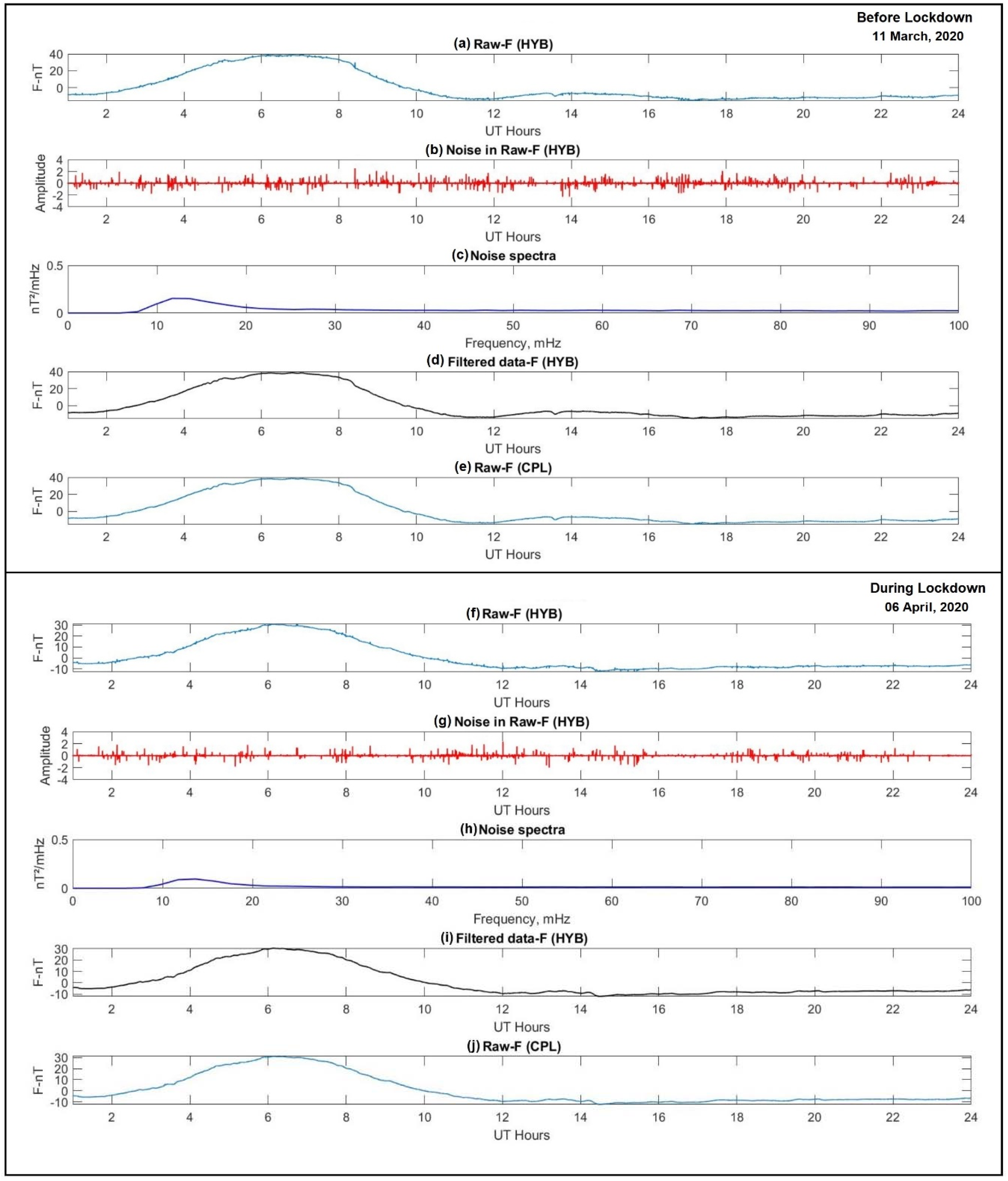
Figure 5 and
Figure 6 show the details of the raw and filtered data before and during the lockdown period from the HYB Observatory. From
Figure 5a,b,f,g and
Figure 6a,b,f,g, a noticeable difference is observed in the occurrence frequency of spikes in the Z and F components before and during the lockdown period. Even though the amplitude was found to be in the range of ±2.5 nT in the Z and F components, the density distribution and frequency of spikes were significantly reduced in the lockdown period when compared to before lockdown. A frequency peak was observed in the noise spectra at 11 mHz in the Z and F components before lockdown and during the lockdown period, and the same frequency peak was noticed with reduced power intensity during the lockdown period in both the components (
Figure 5c,h and
Figure 6c,h).
Figure 5d,i and
Figure 6d,i show the raw signal after removing the noise with a low-pass Butterworth filter with a lower cut-off frequency of 0.01 Hz in the Z and F components.
Figure 5e,j and
Figure 6e,j show the 1 Hz raw signal of the Z and F components from the CPL Observatory. Comparing
Figure 5d,i with
Figure 5e,j, and
Figure 6d,i with
Figure 6e,j, shows that the filtered data are consistent with the raw data from CPL, after removing the remaining sources of anthropogenic noise on the Z and F components at the HYB Observatory.
We also attempted to identify the effect of vehicular noise on the H and D components from the HYB Observatory before and during the lockdown period, and our analysis shows that a negligible difference was observed in the occurrence frequency of spikes, both in the H and D components, before and during the lockdown period, within the range of ±0.03 nT. As observed in the Z and F components, we also observed peaks in the noise spectra at 11 mHz in the H and D components during and before the lockdown period at the HYB Observatory. We also compared the 1 Hz trends of the HYB H and D components with CPL and found that these trends are consistent.
To strengthen our observations with the filtered data for the Z and F components from HYB, we subtracted the corresponding variations from CPL for the days before and during lockdown periods, and the linear trend shows good synchronicity between the observatories. Further, a small deviation of 1.5 nT was observed from the zero crossing line in all the components, which could be due to the distance between the observatories, followed by different geological constraints.
4. Discussion
To estimate the influence of vehicular noise on the 1 Hz measurements of the Z and F data at the HYB Observatory, we analyzed 100 days of data before and during lockdown. Raw variations in Z and F before and during lockdown showed quantifiable differences in the noise levels, with a reduction, to more than half, in the occurrence frequency of spikes. The spike amplitudes of first differences reduced from ±4 nT before lockdown to ±2.5 nT during lockdown in both Z and F.
A noticeable difference is observed in the occurrence frequency of spikes and the distribution density of spikes, which decreased in both the Z and F components during the lockdown period. We observed that the noise had an amplitude of about 8 nT in the raw data of the Z and F components before lockdown and 4 nT during lockdown, when there was no vehicular movement or metro rail. Similarly, at the KEL station (South Moravia), which is 25 m away from the local street, 5–10 nT spikes in the data were observed, attributable to the vehicle movements. Spike amplitudes increase for vans and buses; furthermore, a clear correlation between the spikes and traffic is established by experimental recording using another instrument placed 5 m away from the variometer and closer to the street [
11]). Ref. [
12] reported that at the EBR Observatory (Spain), which was located 0.5 km away from the railway, there were perturbations of about 3 nT and 15 nT in the H and Z components, similar to the effects of anthropogenic noise in the Z component noticed at HYB. In addition, comparing the EBR data with the SPT and AQU stations, which are located in noise-free places, 100 km and 200 km from EBR, respectively, magnetic disturbances appear in the EBR data, but not at the other two observatories, and are statistically estimated to be 89% due to train movements and 11% due to other sources. Similarly, at HYB, the noise was reduced by 60% during lockdown, in the complete absence of metro rail and all vehicular movement; the remaining 40% of noise would be due to the power lines and power station, which are at a distance of 500 m–1 km.
Ref. [
6] identified the influence of two DC power lines, Baltic Cable, operated by Baltic Cable AB, and Kontek, operated by Energinet (
https://en.energinet.dk/) (accessed on 27 November, 2021), on magnetic H and Z elements at Brorfelde (BFE) Geomagnetic Observatory, and found that the H component is increased by about 0.0040 nT per megawatt of increased power by Baltic Cable, and about 0.0022 nT per ampere of increased current by Kontek Cable. The Z component is decreased by about 0.0013 nT for every megawatt of power increase at Baltic Cable, and by about 0.0016 nT for every ampere of current increase at Kontek Cable. Ref. [
8] discussed the noise signatures of planes in the geomagnetic data during take-offs and landings (for a few minutes noticed perturbances in the geomagntic measurements about a few nT) which was about 100 m away from the new Easter Island observatory located at the end of Mataveri airport.
Ref. [
13] identified the noise in the Duronia (DUR) Observatory data during 2018 by computing the signal-to-noise ratio (SNR) on hourly averaged power spectra of both horizontal components (H and D). The observed noise peak at DUR during morning hours was ascribed to the contribution of Pc3–Pc4, as well the contribution of higher levels of local noise in the data. Therefore, the observed peak at 11 mHz in the Z and F components during and before the lockdown periods (
Figure 5c,h and
Figure 6c,h), as well as in the H and D components (not shown here) at the HYB Observatory, is probably due to the presence of residual signal (noise + ULF waves), which is a well-known behavior in the frequency range Pc3–4 (7–100 mHz). The contribution of these two components is difficult to discriminate.


