
RoiSeg: An Effective Moving Object Segmentation Approach Based on Region-of-Interest with Unsupervised Learning


Abstract
:1. Introduction
- We propose RoiSeg, an effective object segmentation approach based on ROI, which utilizes unsupervised learning method to achieve automatic segmentation of moving objects. RoiSeg not only effectively handles ambient lighting changes, fog, salt and pepper noise, but also has a good ability to deal with camera jitter and windy scenes.
- We hypothesize the central n*n pixels as the ROI and simplify the foreground segmentation into a classification problem based on ROI. In addition, we propose an automatic generation method to produce the training samples and implement an online sample classifier to compensate the imbalance of different classes, respectively.
- We also conduct extensive experiments to evaluate the performance of RoiSeg and the experimental results demonstrate that RoiSeg is more accurate and faster compared with other segmentation algorithms.
2. Related Work
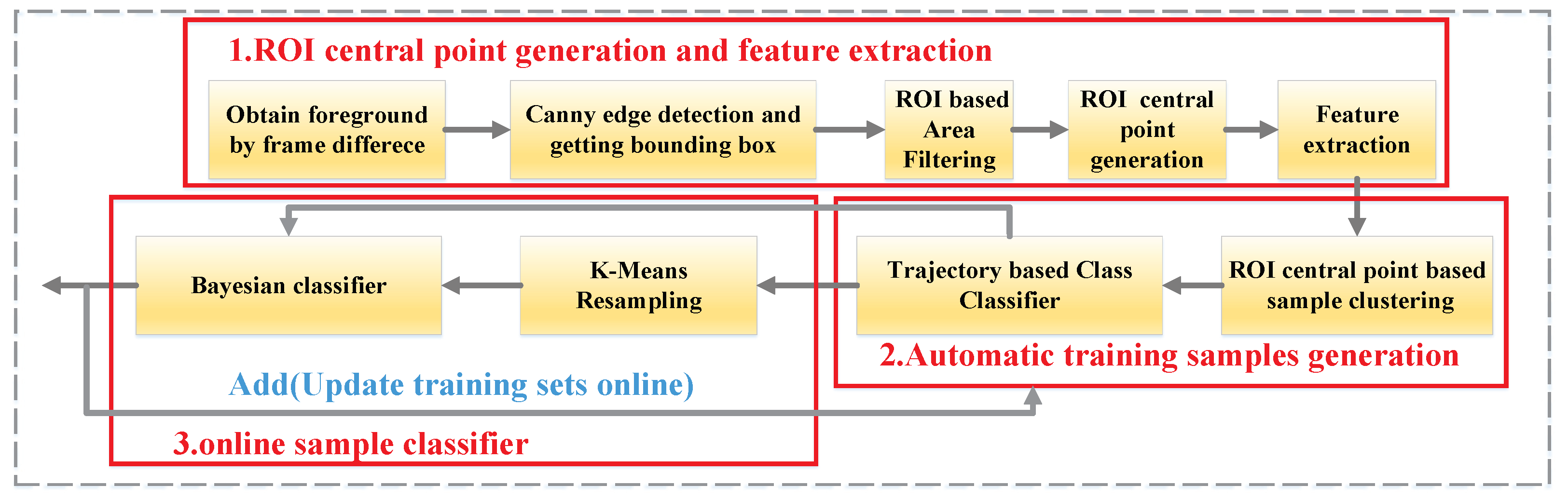
3. Design of RoiSeg
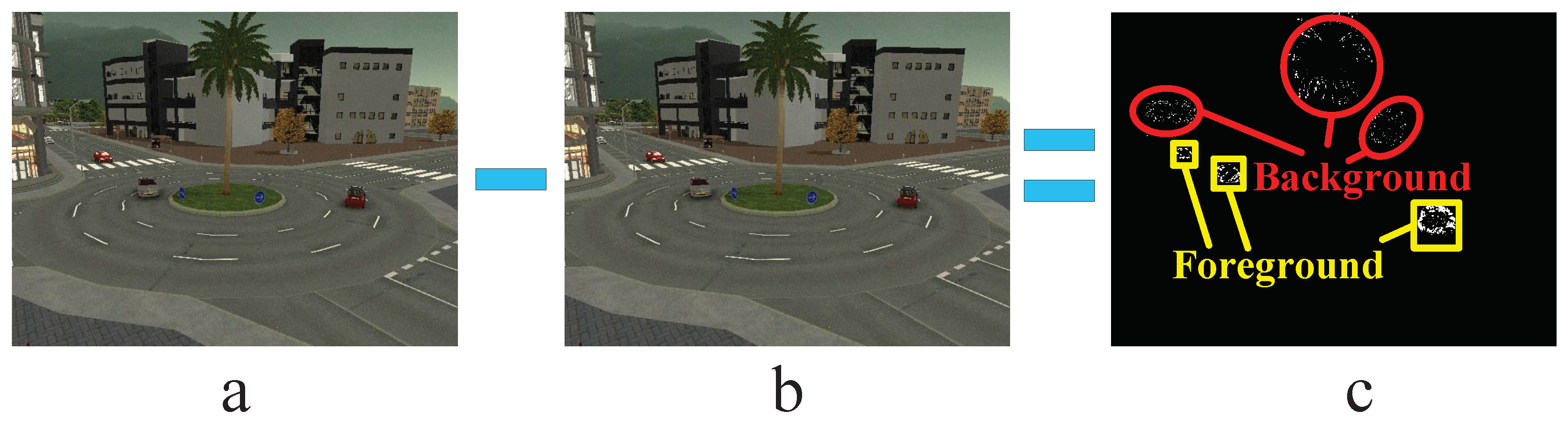
3.1. ROI-Central-Point Generation
3.2. ROI-Based Noise Filter
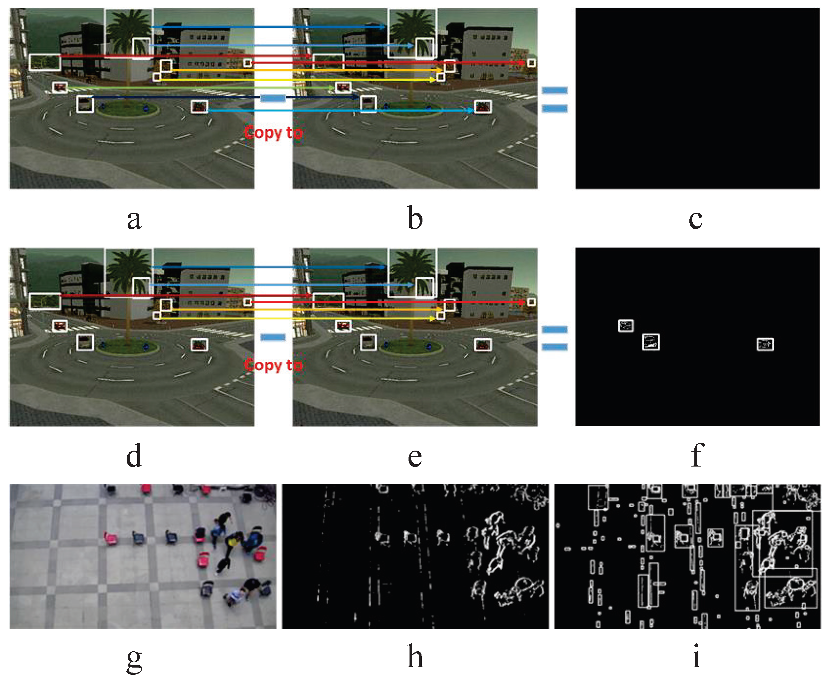
3.3. Automatic Training-Sample Generation
3.3.1. ROI Pooling and Feature Extraction
3.3.2. ROI Central Point Based Sample Clustering
3.3.3. Trajectory Based Class Classifier
3.4. Online Sample Classifier
3.4.1. Imbalance Compensation
3.4.2. Online Sample Updating
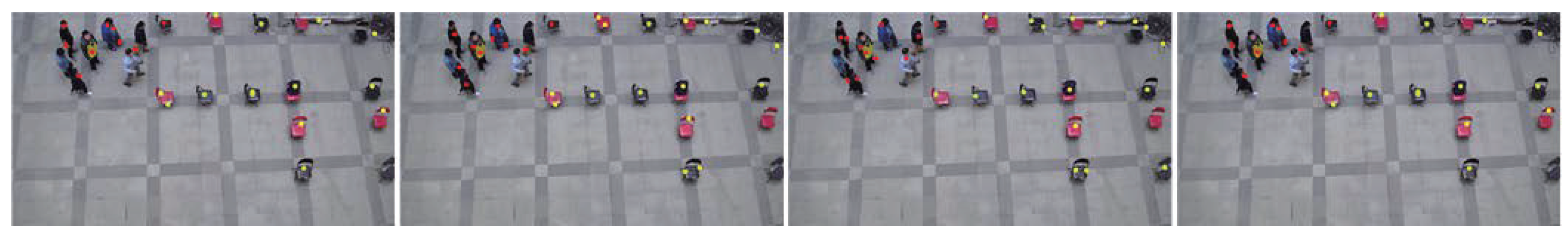
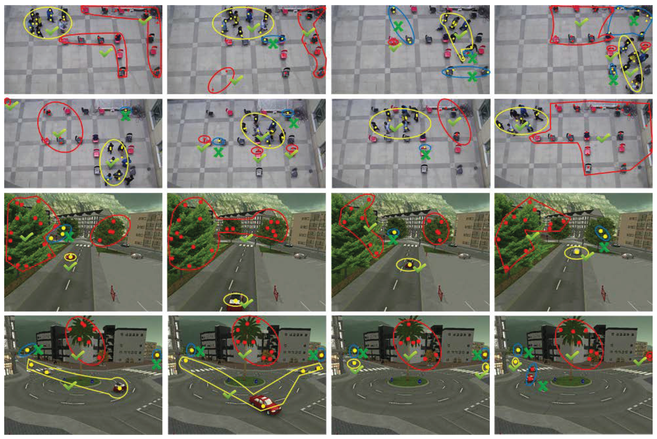
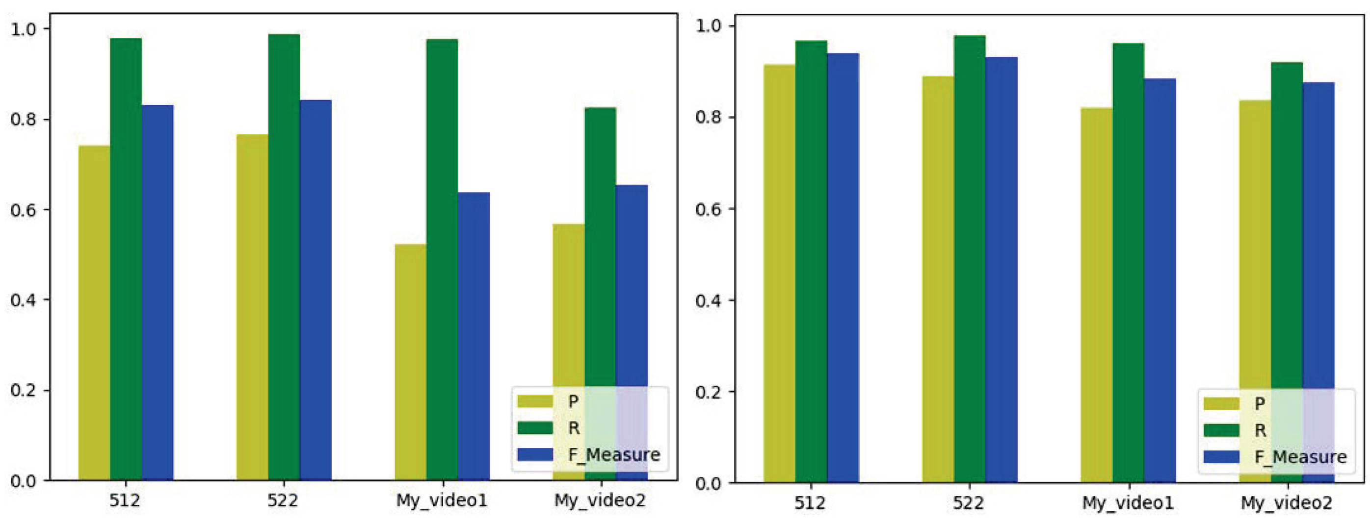
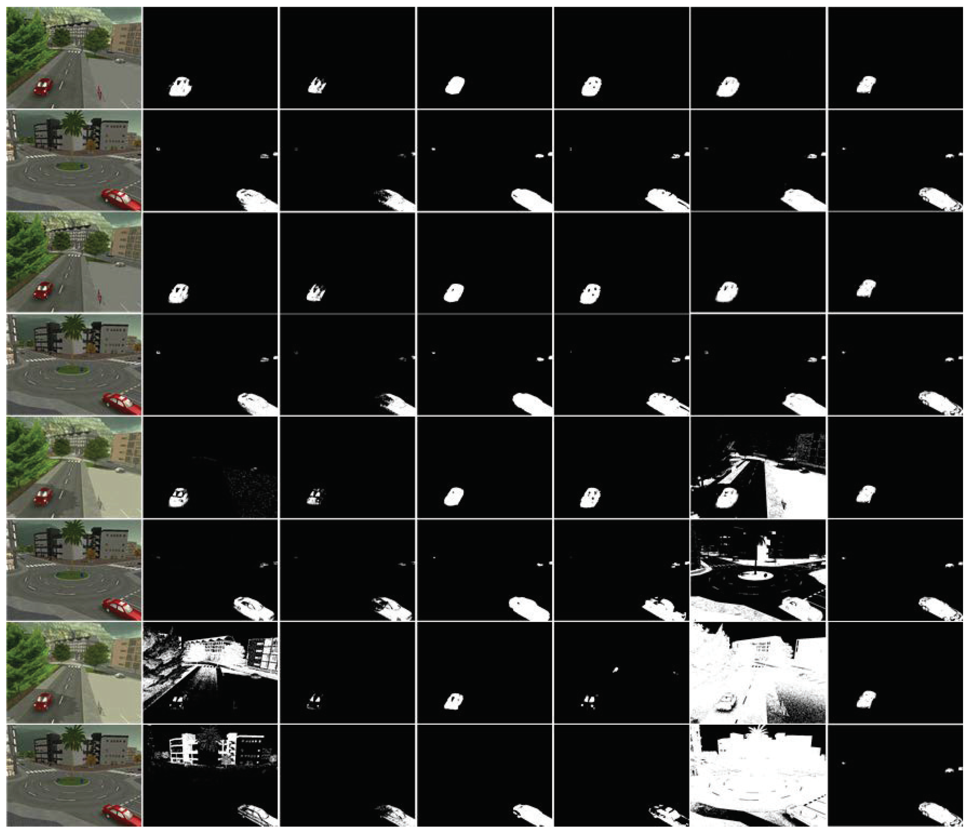
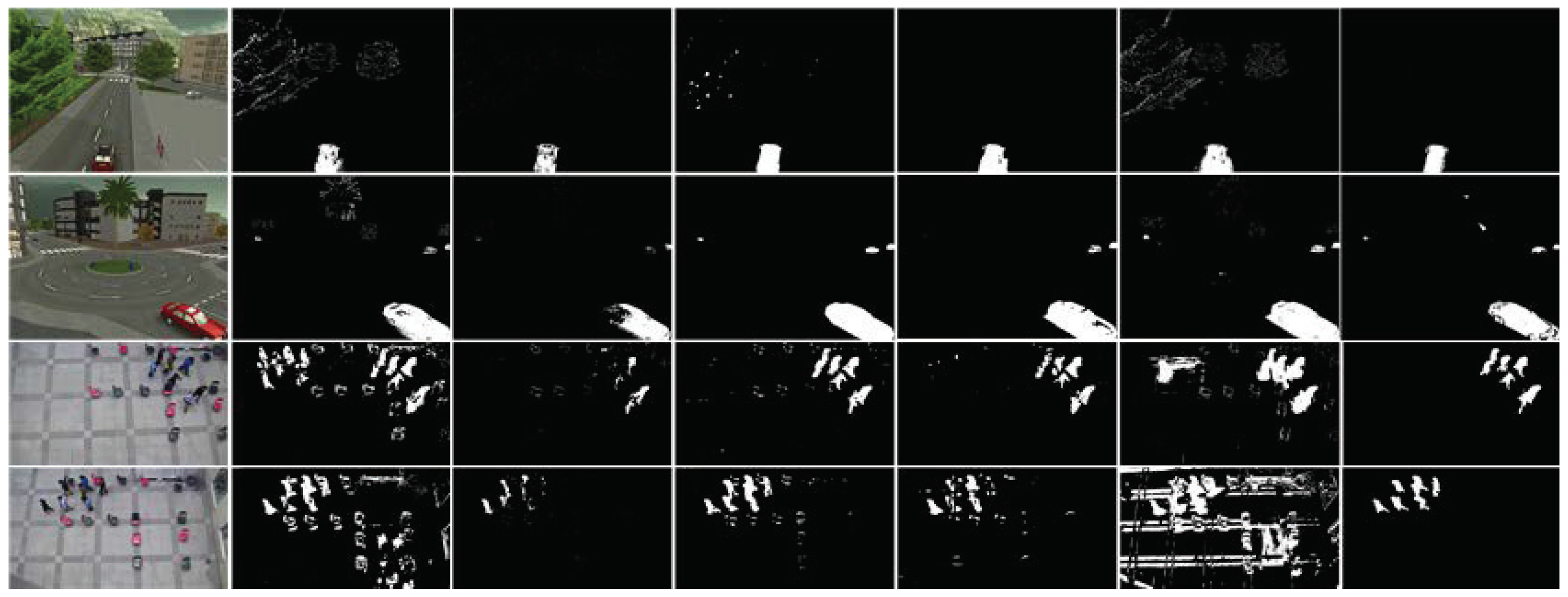
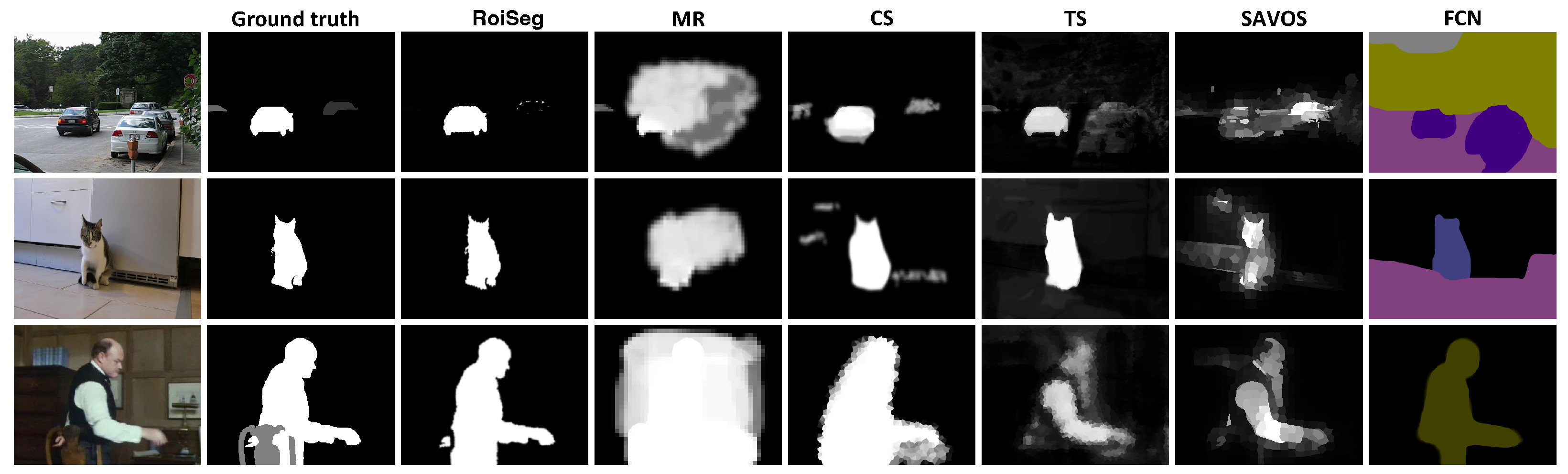
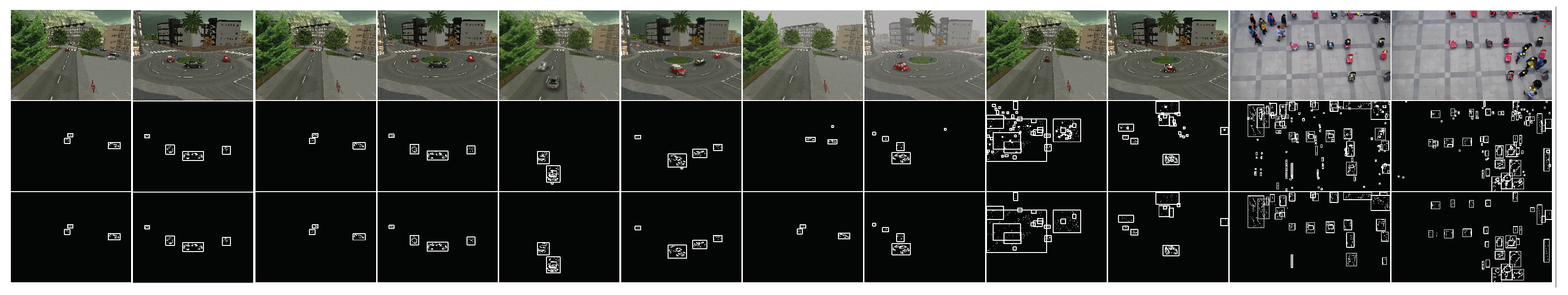
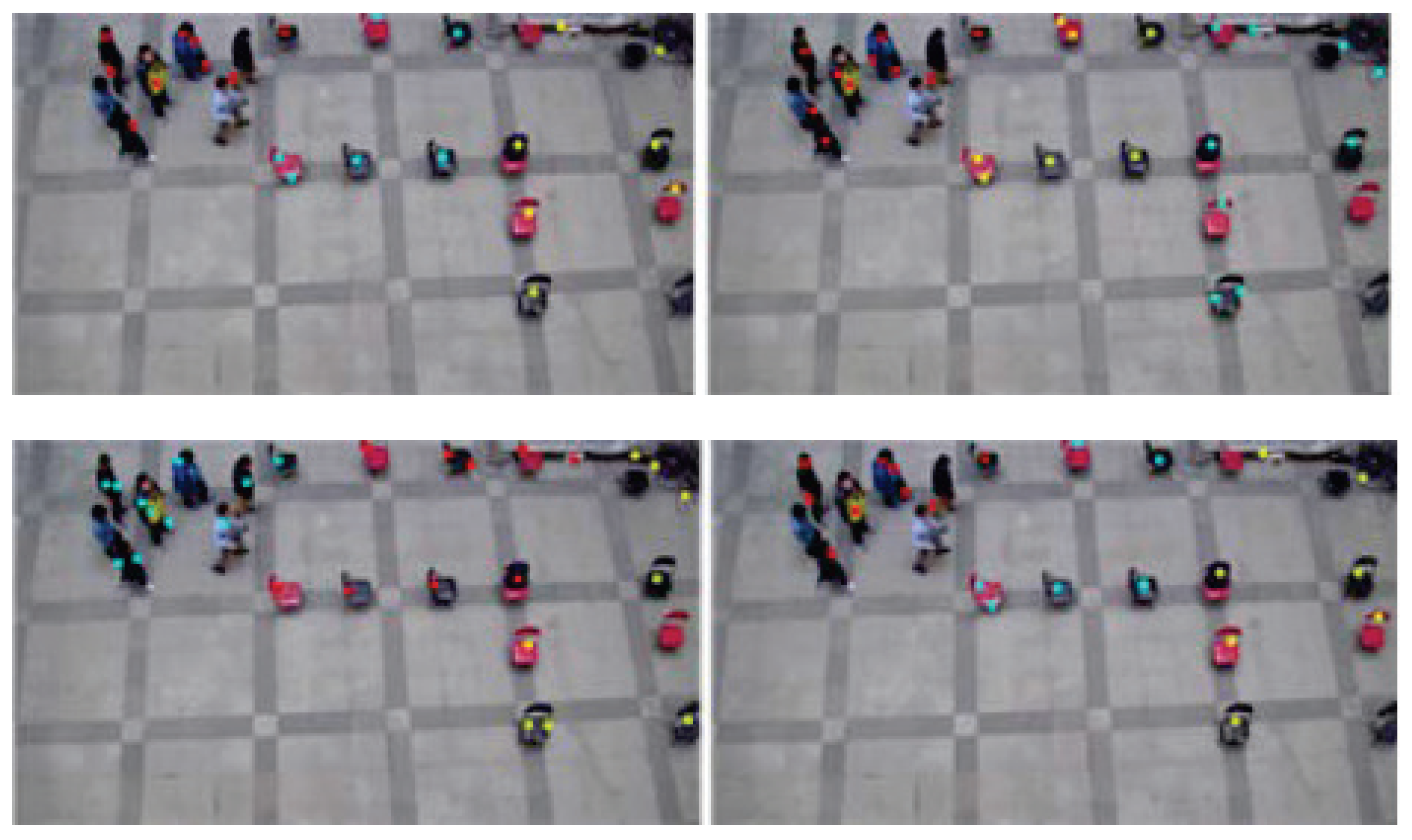
4. Evaluation
5. Conclusions and Future Work
Author Contributions
Funding
Institutional Review Board Statement
Informed Consent Statement
Data Availability Statement
Conflicts of Interest
References
- Agrawal, S.; Natu, P. Segmentation of Moving Objects using Numerous Background Subtraction Methods for Surveillance Applications. Int. J. Innov. Technol. Explor. Eng. (IJITEE) 2020, 9, 2553–2563. [Google Scholar]
- Qu, Z.; Chen, Z. An intelligent vehicle image segmentation and quality assessment model. Future Gener. Comput. Syst. (FGCS) 2021, 117, 426–432. [Google Scholar] [CrossRef]
- Li, L.; Wang, Z.; Hu, Q.; Dong, Y. Adaptive Nonconvex Sparsity Based Background Subtraction for Intelligent Video Surveillance. IEEE Trans. Ind. Inform. (TII) 2020, 17, 4168–4178. [Google Scholar] [CrossRef]
- Garcia-Garcia, B.; Bouwmans, T.; Silva, A.J.R. Background subtraction in real applications: Challenges, current models and future directions. Comput. Sci. Rev. 2020, 35, 100204. [Google Scholar] [CrossRef]
- Kalsotra, R.; Arora, S. Background subtraction for moving object detection: Explorations of recent developments and challenges. Vis. Comput. 2021. [Google Scholar] [CrossRef]
- Sultana, M.; Mahmood, A.; Bouwmans, T.; Jung, S.K. Dynamic background subtraction using least square adversarial learning. In Proceedings of the 2020 IEEE International Conference on Image Processing (ICIP), Abu Dhabi, United Arab Emirates, 25–28 October 2020; pp. 3204–3208. [Google Scholar]
- Liu, X.; Van De Weijer, J.; Bagdanov, A.D. Exploiting Unlabeled Data in CNNS by Self-supervised Learning to Rank. IEEE Trans. Pattern Anal. Mach. Intell. (TPAMI) 2019, 41, 1862–1878. [Google Scholar] [CrossRef] [Green Version]
- Prasad, D.K.; Prasath, C.K.; Rajan, D.; Rachmawati, L.; Rajabally, E.; Quek, C. Object Detection in a Maritime Environment: Performance Evaluation of Background Subtraction Methods. IEEE Trans. Intell. Transp. Syst. (TITS) 2018, 20, 1787–1802. [Google Scholar] [CrossRef]
- Zhao, C.; Sain, A.; Qu, Y.; Ge, Y.; Hu, H. Background Subtraction Based on Integration of Alternative Cues in Freely Moving Camera. IEEE Trans. Circuits Syst. Video Technol. (TCSVT) 2018, 29, 1933–1945. [Google Scholar] [CrossRef]
- Chen, Y.Q.; Sun, Z.L.; Lam, K.M. An Effective Subsuperpixel-Based Approach for Background Subtraction. IEEE Trans. Ind. Electron. (TIE) 2019, 67, 601–609. [Google Scholar] [CrossRef]
- Huang, L.; Fu, Y.; Chen, R.; Yang, S.; Qiu, H.; Wu, X.; Zhao, S.; Gu, Y.; Li, P. SNR-adaptive OCT Angiography Enabled by Statistical Characterization of Intensity and Decorrelation with Multi-variate Time Series Model. IEEE Trans. Med. Imaging (TIP) 2019, 38, 2695–2704. [Google Scholar] [CrossRef] [Green Version]
- Xue, Z.; Yuan, X.; Yang, Y. Denoising-Based Turbo Message Passing for Compressed Video Background Subtraction. IEEE Trans. Image Process. (TIP) 2021, 30, 2682–2696. [Google Scholar] [CrossRef] [PubMed]
- Stauffer, C.; Grimson, W.E.L. Adaptive Background Mixture Models for Real-time Tracking. In Proceedings of the IEEE Computer Society Conference on Computer Vision and Pattern Recognition (CVPR), Fort Collins, CO, USA, 23–25 June 1999; Volume 2, pp. 246–252. [Google Scholar]
- Culibrk, D.; Marques, O.; Socek, D.; Kalva, H.; Furht, B. Neural Network Approach to Background Modeling for Video Object Segmentation. IEEE Trans. Neural Netw. (TNN) 2007, 18, 1614–1627. [Google Scholar] [CrossRef] [PubMed]
- Yu, T.; Zhang, C.; Cohen, M.; Rui, Y.; Wu, Y. Monocular Video Foreground/Background Segmentation by Tracking Spatial-color Gaussian Mixture Models. In Proceedings of the IEEE Workshop on Motion and Video Computing (WMVC), Austin, TX, USA, 23–24 February 2007; pp. 5–13. [Google Scholar]
- Gallego, J.; Pardas, M.; Haro, G. Bayesian Foreground Segmentation and Tracking using Pixel-wise Background Model and Region Based Foreground Model. In Proceedings of the IEEE International Conference on Image Processing (ICIP), Cairo, Egypt, 7–10 November 2009; pp. 3205–3208. [Google Scholar]
- Cuevas, C.; Garcia, N. Efficient Moving Object Detection for Lightweight Applications on Smart Cameras. IEEE Trans. Circuits Syst. Video Technol. (TCSVT) 2013, 23, 1–14. [Google Scholar] [CrossRef]
- Wu, J.; Dong, M.; Ota, K.; Li, J.; Guan, Z. Big Data Analysis-based Secure Cluster Management for Optimized Control Plane in Software-defined Networks. IEEE Trans. Netw. Serv. Manag. (TNSM) 2018, 15, 27–38. [Google Scholar] [CrossRef] [Green Version]
- Afshang, M.; Dhillon, H.S. Poisson Cluster Process Based Analysis of HetNets with Correlated User and Base Station Locations. IEEE Trans. Wirel. Commun. (TWC) 2018, 17, 2417–2431. [Google Scholar] [CrossRef]
- Bu, Z.; Li, H.J.; Zhang, C.; Cao, J.; Li, A.; Shi, Y. Graph K-means Based on Leader Identification, Dynamic Game, and Opinion Dynamics. IEEE Trans. Knowl. Data Eng. (TKDE) 2019, 32, 1348–1361. [Google Scholar] [CrossRef]
- Seiffert, C.; Khoshgoftaar, T.M.; Van Hulse, J.; Napolitano, A. RUSBoost: A Hybrid Approach to Alleviating Class Imbalance. IEEE Trans. Syst. Man Cybern.-Part A Syst. Hum. 2009, 40, 185–197. [Google Scholar] [CrossRef]
- Nidheesh, N.; Nazeer, K.A.; Ameer, P. An Enhanced Deterministic K-Means Clustering Algorithm for Cancer Subtype Prediction from Gene Expression Data. Comput. Biol. Med. 2017, 91, 213–221. [Google Scholar] [CrossRef]
- Zhou, Y.; Rangarajan, A.; Gader, P.D. A Gaussian Mixture Model Representation of Endmember Variability in Hyperspectral Unmixing. IEEE Trans. Image Process. (TIP) 2018, 27, 2242–2256. [Google Scholar] [CrossRef] [Green Version]
- Wang, C.; Yan, Z.; Pedrycz, W.; Zhou, M.; Li, Z. A Weighted Fidelity and Regularization-based Method for Mixed or Unknown Noise Removal from Images on Graphs. IEEE Trans. Image Process. (TIP) 2020, 29, 5229–5243. [Google Scholar] [CrossRef]
- Jiang, L.; Zhang, L.; Li, C.; Wu, J. A Correlation-based Feature Weighting Filter for Naive Bayes. IEEE Trans. Knowl. Data Eng. (TKDE) 2018, 31, 201–213. [Google Scholar] [CrossRef]
- Kim, S.B.; Han, K.S.; Rim, H.C.; Myaeng, S.H. Some Effective Techniques for Naive Bayes Text Classification. IEEE Trans. Knowl. Data Eng. (TKDE) 2006, 18, 1457–1466. [Google Scholar]
- Wu, D.; Jiang, Z.; Xie, X.; Wei, X.; Yu, W.; Li, R. LSTM Learning with Bayesian and Gaussian Processing for Anomaly Detection in Industrial IoT. IEEE Trans. Ind. Inform. (TII) 2019, 16, 5244–5253. [Google Scholar] [CrossRef] [Green Version]
- Yerima, S.Y.; Sezer, S. DroidFusion: A Novel Multilevel Classifier Fusion Approach for Android Malware Detection. IEEE Trans. Cybern. 2018, 49, 453–466. [Google Scholar] [CrossRef] [PubMed]
- Yu, H.; Yang, X.; Zheng, S.; Sun, C. Active Learning from Imbalanced Data: A Solution of Online Weighted Extreme Learning Machine. IEEE Trans. Neural Netw. Learn. Syst. (TNNLS) 2018, 30, 1088–1103. [Google Scholar] [CrossRef]
- Galar, M. A Review on Ensembles for the Class Imbalance Problem: Bagging-, Boosting-, and Hybrid-Based Approaches. IEEE Trans. Syst. Man Cybern. Part C Appl. Rev. 2012, 42, 463–484. [Google Scholar] [CrossRef]
- Beyan, C.; Fisher, R. Classifying Imbalanced Data Sets using Similarity Based Hierarchical Decomposition. Pattern Recognit. 2015, 48, 1653–1672. [Google Scholar] [CrossRef] [Green Version]
- Batista, G.E.; Prati, R.C.; Monard, M.C. A Study of the Behavior of Several Methods for Balancing Machine Learning Training Data. ACM Sigkdd Explor. Newsl. 2004, 6, 20–29. [Google Scholar] [CrossRef]
- Lin, W.C.; Tsai, C.F.; Hu, Y.H.; Jhang, J.S. Clustering-based Undersampling in Class-imbalanced Data. Inf. Sci. 2017, 409, 17–26. [Google Scholar] [CrossRef]
- Hu, S.; Liang, Y.; Ma, L.; He, Y. MSMOTE: Improving Classification Performance When Training Data is Imbalanced. In Proceedings of the International Workshop on Computer Science and Engineering, Qingdao, China, 28–30 October 2009; Volume 2, pp. 13–17. [Google Scholar]
- Zhang, X.; Zhu, C.; Wu, H.; Liu, Z.; Xu, Y. An Imbalance Compensation Framework for Background Subtraction. IEEE Trans. Multimed. (TMM) 2017, 19, 2425–2438. [Google Scholar] [CrossRef]
- Cui, Y.; Wang, Q.; Yuan, H.; Song, X.; Hu, X.; Zhao, L. Relative Localization in Wireless Sensor Networks for Measurement of Electric Fields under HVDC Transmission Lines. Sensors 2015, 15, 3540–3564. [Google Scholar] [CrossRef] [PubMed] [Green Version]
- He, M.; Luo, H.; Chang, Z.; Hui, B. Pedestrian Detection with Semantic Regions of Interest. Sensors 2017, 17, 2699. [Google Scholar] [CrossRef] [PubMed] [Green Version]
- Sobral, A.; Vacavant, A. A Comprehensive Review of Background Subtraction Algorithms Evaluated with Synthetic and Real Videos. Comput. Vis. Image Underst. (CVIU) 2014, 122, 4–21. [Google Scholar] [CrossRef]
- Tsai, D.; Flagg, M.; Nakazawa, A.; Rehg, J.M. Motion coherent tracking using multi-label MRF optimization. Int. J. Comput. Vis. (IJCV) 2012, 100, 190–202. [Google Scholar] [CrossRef]
- Yang, C.; Zhang, L.; Lu, H.; Ruan, X.; Yang, M.H. Saliency detection via graph-based manifold ranking. In Proceedings of the IEEE Conference on Computer Vision and Pattern Recognition (CVPR), Portland, OR, USA, 23–28 June 2013; pp. 3166–3173. [Google Scholar]
- Wang, W.; Shen, J.; Yang, R.; Porikli, F. Saliency-aware video object segmentation. IEEE Trans. Pattern Anal. Mach. Intell. (TPAMI) 2017, 40, 20–33. [Google Scholar] [CrossRef] [PubMed]
- Fu, H.; Cao, X.; Tu, Z. Cluster-based co-saliency detection. IEEE Trans. Image Process. (TIP) 2013, 22, 3766–3778. [Google Scholar] [CrossRef] [Green Version]
- Zhou, F.; Bing Kang, S.; Cohen, M.F. Time-mapping using space-time saliency. In Proceedings of the IEEE Conference on Computer Vision and Pattern Recognition (CVPR), Columbus, OH, USA, 23–28 June 2014; pp. 3358–3365. [Google Scholar]
- Zhang, D.; Javed, O.; Shah, M. Video object segmentation through spatially accurate and temporally dense extraction of primary object regions. In Proceedings of the IEEE Conference on Computer Vision and Pattern Recognition (CVPR), Portland, OR, USA, 23–28 June 2013; pp. 628–635. [Google Scholar]
- Papazoglou, A.; Ferrari, V. Fast object segmentation in unconstrained video. In Proceedings of the IEEE International Conference on Computer Vision (ICCV), Sydney, NSW, Australia, 1–8 December 2013; pp. 1777–1784. [Google Scholar]
- Long, J.; Shelhamer, E.; Darrell, T. Fully convolutional networks for semantic segmentation. In Proceedings of the IEEE Conference on Computer Vision and Pattern Recognition (CVPR), Boston, MA, USA, 7–12 June 2015; pp. 3431–3440. [Google Scholar]
- Brox, T.; Malik, J. Object segmentation by long term analysis of point trajectories. In Proceedings of the European Conference on Computer Vision (ECCV), Heraklion, Greece, 5–11 September 2010; pp. 282–295. [Google Scholar]
- Jang, W.D.; Lee, C.; Kim, C.S. Primary object segmentation in videos via alternate convex optimization of foreground and background distributions. In Proceedings of the IEEE Conference on Computer Vision and Pattern Recognition (CVPR), Las Vegas, NV, USA, 27–30 June 2016; pp. 696–704. [Google Scholar]
- Li, F.; Kim, T.; Humayun, A.; Tsai, D.; Rehg, J.M. Video segmentation by tracking many figure-ground segments. In Proceedings of the IEEE International Conference on Computer Vision (ICCV), Sydney, NSW, Australia, 1–8 December 2013; pp. 2192–2199. [Google Scholar]
- Wen, L.; Du, D.; Lei, Z.; Li, S.Z.; Yang, M.H. Jots: Joint online tracking and segmentation. In Proceedings of the IEEE Conference on Computer Vision and Pattern Recognition (CVPR), Boston, MA, USA, 7–12 June 2015; pp. 2226–2234. [Google Scholar]
- Tsai, Y.H.; Yang, M.H.; Black, M.J. Video segmentation via object flow. In Proceedings of the IEEE Conference on Computer Vision and Pattern Recognition (CVPR), Las Vegas, NV, USA, 27–30 June 2016; pp. 3899–3908. [Google Scholar]
- Xiao, F.; Jae Lee, Y. Track and segment: An iterative unsupervised approach for video object proposals. In Proceedings of the IEEE Conference on Computer Vision and Pattern Recognition (CVPR), Las Vegas, NV, USA, 27–30 June 2016; pp. 933–942. [Google Scholar]
- Everingham, M.; Van Gool, L.; Williams, C.; Winn, J.; Zisserman, A. The PASCAL Visual Object Classes Challenge 2011 (VOC 2011) Results. Available online: http://www.pascal-network.org/challenges/VOC/voc2011/workshop/index.html (accessed on 2 January 2022).


| Dataset | 112 | 122 | 212 | 222 | 312 | 322 | 412 | 422 | 512 | 522 | My_video1 | My_video2 |
|---|---|---|---|---|---|---|---|---|---|---|---|---|
| ∞ | ∞ | ∞ | ∞ | ∞ | ∞ | ∞ | ∞ | 0.0489 | 0.144 | 0.342 | 0.314 |
| Sequences | Description | Size |
|---|---|---|
| 112 | Cloudy, without acquisition noise, as normal mode | 640 × 480 |
| 122 | 640 × 480 | |
| 212 | Cloudy, with salt and pepper noise during the whole sequence | 640 × 480 |
| 222 | 640 × 480 | |
| 312 | Sunny, with noise, generating moving cast shadows | 640 × 480 |
| 322 | 640 × 480 | |
| 412 | Foggy, with noise, making both background and foreground hard to analyze | 640 × 480 |
| 422 | 640 × 480 | |
| 512 | Wind, with noise, producing a moving background | 640 × 480 |
| 522 | 640 × 480 | |
| My_video1 | Camera jitter | 1280 × 720 |
| My_video2 | 1280 × 720 |
| Video Sequences | 112 | 122 | 212 | 222 | 312 | 322 | 412 | 422 | 512 | 522 | My_video1 | My_video2 |
|---|---|---|---|---|---|---|---|---|---|---|---|---|
| Number of Video clips | 1502 | 1503 | 1499 | 1499 | 1499 | 1501 | 1499 | 1499 | 1499 | 1499 | 390 | 390 |
| number of pixels in a bounding box | 304 | 218 | 304 | 218 | 304 | 218 | 304 | 218 | 304 | 218 | 1000 | 1000 |
| Total area of frame covered by bounding boxes for noise (%) | 0.1 | 0.07 | 0.1 | 0.07 | 0.1 | 0.07 | 0.1 | 0.07 | 0.1 | 0.07 | 0.1 | 0.1 |
| BMC Sequences | DPWren GABGS | Mixture Of Gaussian V1BGS | MultiLayer BGS | Pixel Based Adaptive Segmenter | LBAdaptive SOM | Proposed RoiSeg | ||||||||||||||||||
|---|---|---|---|---|---|---|---|---|---|---|---|---|---|---|---|---|---|---|---|---|---|---|---|---|
| P | R | F | FPS | P | R | F | FPS | P | R | F | FPS | P | R | F | FPS | P | R | F | FPS | P | R | F | FPS | |
| 112 | 0.87 | 0.87 | 0.87 | 70.2 | 0.96 | 0.74 | 0.84 | 89.3 | 0.92 | 0.95 | 0.93 | 5 | 0.88 | 0.9 | 0.89 | 15.6 | 0.86 | 0.92 | 0.89 | 20.6 | 0.89 | 0.93 | 0.91 | 115 |
| 122 | 0.91 | 0.87 | 0.89 | 77.6 | 0.96 | 0.7 | 0.8 | 70.5 | 0.91 | 0.94 | 0.93 | 2.2 | 0.9 | 0.88 | 0.89 | 13.2 | 0.88 | 0.93 | 0.9 | 22.3 | 0.91 | 0.94 | 0.92 | 120.6 |
| 212 | 0.92 | 0.86 | 0.89 | 58.3 | 0.97 | 0.74 | 0.84 | 70.3 | 0.94 | 0.94 | 0.94 | 2.5 | 0.89 | 0.89 | 0.89 | 8.2 | 0.79 | 0.77 | 0.78 | 15.5 | 0.89 | 0.93 | 0.91 | 70.6 |
| 222 | 0.93 | 0.86 | 0.9 | 59.2 | 0.96 | 0.7 | 0.81 | 70.6 | 0.94 | 0.93 | 0.93 | 3.5 | 0.9 | 0.87 | 0.89 | 7.6 | 0.89 | 0.92 | 0.91 | 14.2 | 0.91 | 0.94 | 0.92 | 85.1 |
| 312 | 0.65 | 0.78 | 0.71 | 70.4 | 0.98 | 0.68 | 0.8 | 73.8 | 0.96 | 0.87 | 0.91 | 2.4 | 0.88 | 0.87 | 0.87 | 11.2 | 0.52 | 0.84 | 0.64 | 19.2 | 0.89 | 0.93 | 0.91 | 103.2 |
| 322 | 0.89 | 0.78 | 0.83 | 63.2 | 0.95 | 0.65 | 0.77 | 65.9 | 0.94 | 0.85 | 0.89 | 4.3 | 0.9 | 0.8 | 0.85 | 12.3 | 0.54 | 0.85 | 0.66 | 15.1 | 0.91 | 0.94 | 0.92 | 88.3 |
| 412 | 0.53 | 0.76 | 0.62 | 62.1 | 0.98 | 0.69 | 0.81 | 87.7 | 0.71 | 0.84 | 0.77 | 3.1 | 0.85 | 0.82 | 0.84 | 11.5 | 0.51 | 0.78 | 0.61 | 13.3 | 0.89 | 0.93 | 0.91 | 98.1 |
| 422 | 0.53 | 0.75 | 0.62 | 69.3 | 0.97 | 0.64 | 0.77 | 75.8 | 0.77 | 0.79 | 0.78 | 3.9 | 0.85 | 0.77 | 0.81 | 10.4 | 0.51 | 0.78 | 0.62 | 15.1 | 0.91 | 0.94 | 0.92 | 85.8 |
| 512 | 0.63 | 0.86 | 0.73 | 73.4 | 0.82 | 0.74 | 0.78 | 76.8 | 0.65 | 0.93 | 0.76 | 4.1 | 0.82 | 0.89 | 0.86 | 14.1 | 0.52 | 0.88 | 0.66 | 18.3 | 0.81 | 0.91 | 0.86 | 102.3 |
| 522 | 0.8 | 0.86 | 0.83 | 70.3 | 0.91 | 0.69 | 0.79 | 72.2 | 0.88 | 0.93 | 0.9 | 3.3 | 0.89 | 0.87 | 0.88 | 12.4 | 0.67 | 0.92 | 0.78 | 21.6 | 0.89 | 0.93 | 0.91 | 99.1 |
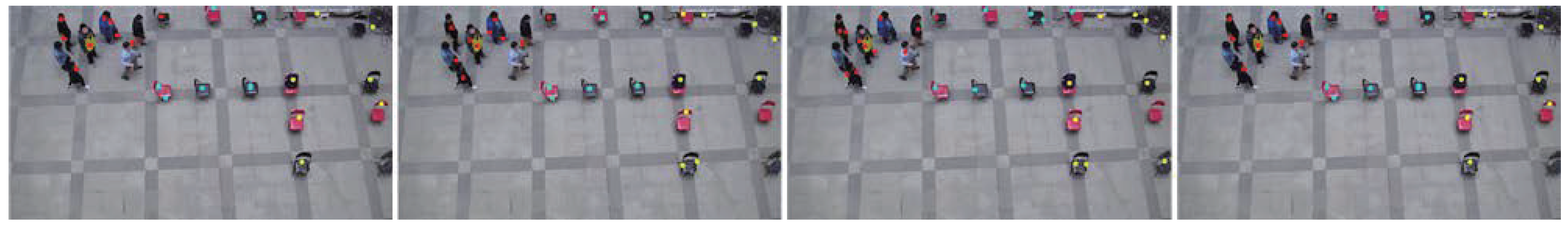
| My_video1 | 0.38 | 0.84 | 0.54 | 12.1 | 0.68 | 0.52 | 0.59 | 16.3 | 0.76 | 0.89 | 0.83 | 0.5 | 0.82 | 0.89 | 0.85 | 5.1 | 0.42 | 0.8 | 0.55 | 6.5 | 0.9 | 0.91 | 0.86 | 42.23 |
| My_video1 | 0.3 | 0.83 | 0.44 | 11.3 | 0.8 | 0.48 | 0.6 | 13.5 | 0.75 | 0.84 | 0.79 | 0.45 | 0.75 | 0.85 | 0.8 | 4.5 | 0.23 | 0.87 | 0.36 | 3.2 | 0.86 | 0.86 | 0.86 | 39.62 |
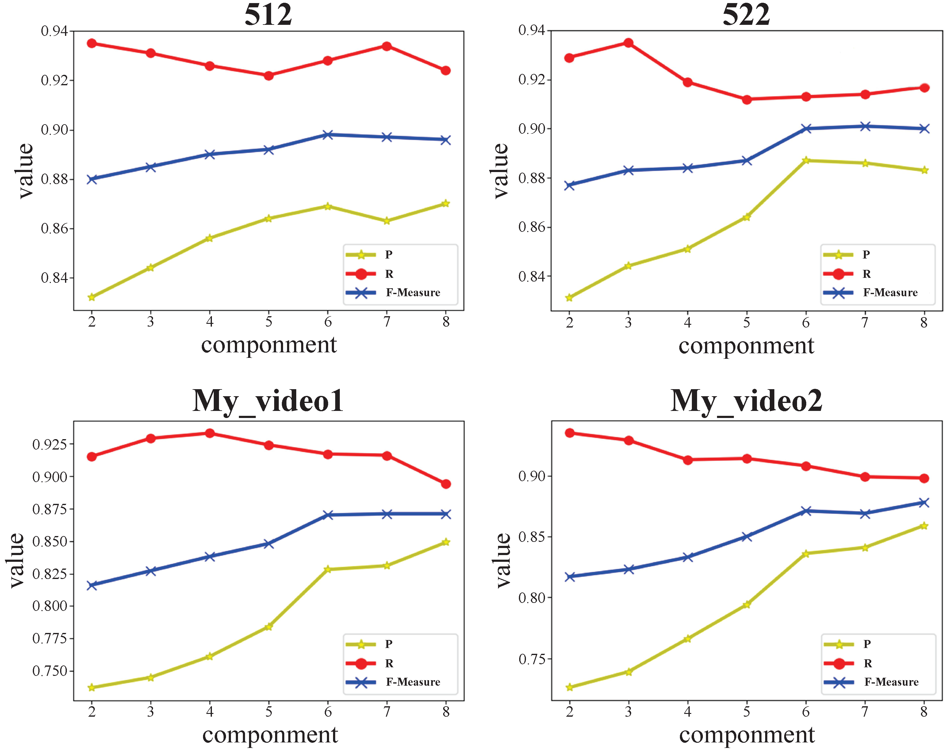
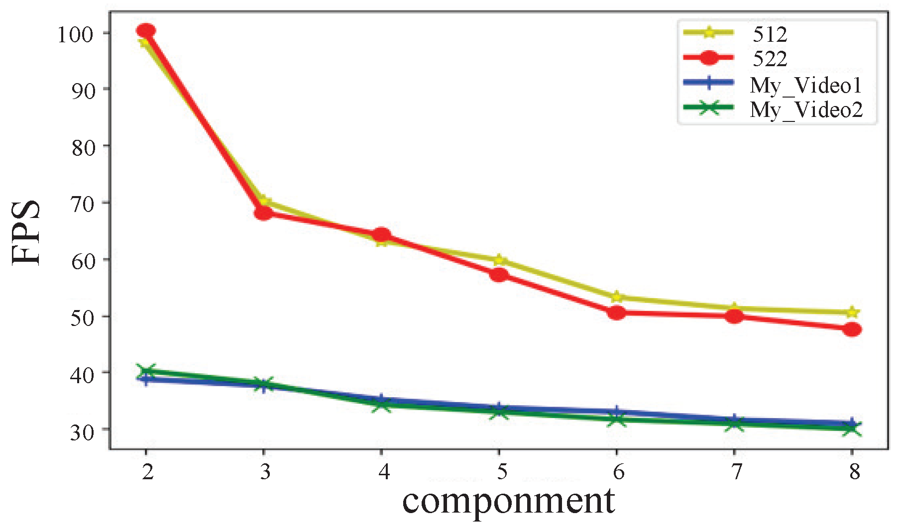
| Dataset | Video Clips | 2 | 3 | 4 | 5 | 6 | 7 | 8 | 9 | 10 |
|---|---|---|---|---|---|---|---|---|---|---|
| 512 | 1499 | 0.528 | 0.683 | 0.856 | 0.914 | 0.924 | 0.919 | 0.903 | 0.839 | 0.789 |
| 522 | 1499 | 0.579 | 0.654 | 0.887 | 0.912 | 0.908 | 0.878 | 0.854 | 0.803 | 0.776 |
| My_video1 | 390 | 0.471 | 0.589 | 0.718 | 0.842 | 0.903 | 0.879 | 0.803 | 0.753 | 0.684 |
| My_video2 | 390 | 0.521 | 0.571 | 0.733 | 0.883 | 0.899 | 0.857 | 0.794 | 0.709 | 0.649 |
| Imbalance Degree | 512 | 522 | Video1 | Video2 |
|---|---|---|---|---|
| 0.184 | 0.538 | 0.421 | 0.523 |
| Video | RoiSeg | [42] | [44] | [45] | [41] | [46] |
|---|---|---|---|---|---|---|
| Bear2 | 63.51 | 87.52 | 21.14 | 86.81 | 70.11 | 88.92 |
| Cars5 | 15.62 | 10.71 | 38.73 | 17.38 | 38.52 | 60.11 |
| Cars9 | 30.17 | 19.55 | 28.92 | 52.44 | 60.08 | 77.82 |
| Cats1 | 78.83 | 19.75 | 81.49 | 83.11 | 85.72 | 70.13 |
| People1 | 58.63 | 56.06 | 64.82 | 53.33 | 68.12 | 77.07 |
| People5 | 55.82 | 10.71 | 84.43 | 51.81 | 56.41 | 73.31 |
| Rabbits2 | 56.01 | 20.41 | 47.81 | 28.32 | 71.06 | 79.12 |
| Avg. | 51.23 | 32.10 | 52.48 | 53.31 | 64.29 | 75.21 |
| Video | Frames | Unsupervised | Supervised | ||||||||
|---|---|---|---|---|---|---|---|---|---|---|---|
| RoiSeg | [47] | [44] | [45] | [48] | [49] | [50] | [41] | [39] | [51] | ||
| Birdfall | 30 | 352 | 217 | 155 | 189 | 144 | 199 | 468 | 140 | 252 | 454 |
| Cheetah | 29 | 776 | 890 | 633 | 806 | 617 | 599 | 1968 | 622 | 1142 | 1217 |
| Girl | 21 | 1253 | 3859 | 1488 | 1698 | 1195 | 1164 | 7595 | 991 | 1304 | 1755 |
| Monkeydog | 71 | 557 | 284 | 365 | 472 | 354 | 322 | 1434 | 350 | 563 | 683 |
| Parachute | 51 | 412 | 855 | 220 | 221 | 200 | 242 | 1113 | 195 | 235 | 502 |
| Avg. | 670 | 1221 | 572 | 677 | 502 | 505 | 2516 | 459 | 699 | 922 | |
| Video | Frames | Unsupervised | Supervised | |||||||
|---|---|---|---|---|---|---|---|---|---|---|
| RoiSeg | [44] | [45] | [52] | [48] | [41] | [50] | [51] | [46] | ||
| Birdfall | 30 | 60.91 | 71.43 | 37.39 | 72.52 | 73.21 | 74.51 | 78.71 | 57.41 | 78.83 |
| Cheetah | 29 | 50.12 | 58.75 | 40.91 | 61.21 | 64.22 | 64.34 | 66.12 | 33.82 | 75.31 |
| Girl | 21 | 70.94 | 81.91 | 71.21 | 86.37 | 86.67 | 88.72 | 84.64 | 87.85 | 88.84 |
| Monkeydog | 71 | 65.21 | 74.24 | 73.58 | 74.07 | 76.12 | 78.04 | 82.15 | 54.35 | 85.65 |
| Parachute | 51 | 90.12 | 93.93 | 88.08 | 95.92 | 94.62 | 94.8 | 94.42 | 94.52 | 95.61 |
| Avg. | 67.46 | 76.05 | 62.23 | 78.02 | 78.97 | 80.08 | 81.21 | 65.59 | 84.85 | |
Publisher’s Note: MDPI stays neutral with regard to jurisdictional claims in published maps and institutional affiliations. |
© 2022 by the authors. Licensee MDPI, Basel, Switzerland. This article is an open access article distributed under the terms and conditions of the Creative Commons Attribution (CC BY) license (https://creativecommons.org/licenses/by/4.0/).
Share and Cite
Zhang, Z.; Pei, Z.; Tang, Z.; Gu, F. RoiSeg: An Effective Moving Object Segmentation Approach Based on Region-of-Interest with Unsupervised Learning. Appl. Sci. 2022, 12, 2674. https://doi.org/10.3390/app12052674
Zhang Z, Pei Z, Tang Z, Gu F. RoiSeg: An Effective Moving Object Segmentation Approach Based on Region-of-Interest with Unsupervised Learning. Applied Sciences. 2022; 12(5):2674. https://doi.org/10.3390/app12052674
Chicago/Turabian StyleZhang, Zeyang, Zhongcai Pei, Zhiyong Tang, and Fei Gu. 2022. "RoiSeg: An Effective Moving Object Segmentation Approach Based on Region-of-Interest with Unsupervised Learning" Applied Sciences 12, no. 5: 2674. https://doi.org/10.3390/app12052674
APA StyleZhang, Z., Pei, Z., Tang, Z., & Gu, F. (2022). RoiSeg: An Effective Moving Object Segmentation Approach Based on Region-of-Interest with Unsupervised Learning. Applied Sciences, 12(5), 2674. https://doi.org/10.3390/app12052674