Design of a Chaotic Trajectory Generator Algorithm for Mobile Robots

Abstract

This paper addresses the problem of designing an algorithm capable of generating chaotic trajectories for mobile robots. In particular, the chaotic behavior is induced in the linear and angular velocities of a differential drive mobile robot by infusing them with the states of the Hénon chaotic map. A possible application of patrolling a work area by using trajectories with chaotic motion in differential drive mobile robots is presented. In this work, obtained numerical and experimental results are reported and analyzed. In addition, two quantitative numerical tests are applied in order to measure the chaoticity of the generated trajectories. With the intention of expanding this work further, we explore the case where multiple mobile robots move simultaneously in the same work area with different trajectories, and the final results are exhaustively analyzed. In addition, experimental results are presented.

1. Introduction

Studies on food searching behavior of animal groups (especially ants) helps in the solution of many problems, primarily optimization problems. Recently, biologists have discovered that ant activity is mostly of a chaotic nature [1].

Research has been carried out on chaotic trajectory design for mobile robots in order to imitate this behavior found in nature. Some researchers have used chaotic systems alongside the behavioral equations of differential drive mobile robots to obtain a mathematical model that causes erratic motion [2]; in other research, the use of a standard map (a well-known discrete two-dimensional chaotic system) to generate a series of chaotic way-points to be followed by robots is presented in [3]. There has been other research [4] that used a chaotic random bit generator. In addition, some research [5] has studied the generation of chaotic behavior in mobile robots while they follow a specified path. Other works [6,7] have studied the emergence of chaotic behavior in mobile robots. Recently, [8] addressed the problem of surveillance from a confined area using a four-engine unmanned aerial vehicle by using chaotic systems to design an unpredictable velocity profile for the quadrotor.

Motivation

One of the main characteristics of a chaotic system is its unpredictability. Applying such a feature to a mobile robot’s trajectory may bring several benefits and possible applications; some of them are as follows: border patrol, dangerous object search (for example, explosives), rescue, and unknown territory exploration, among others.

For example, let us suppose there is a valuable object located in a work area (such as a table or a room). A differential drive mobile robot is used to patrol the area, serving as a security guard for said object. The robot may move in a “predefined” manner, using predictable movement previously programmed (see Figure 1a). Any trespasser could easily predict the path the robot would follow, enabling him to reach the valuable object without being detected by it. However, by using unpredictable trajectories (Figure 1b), it would be technically impossible for the trespasser to reach the object without being detected.

In order to achieve these unpredictable (chaotic) trajectories, some recent studies [9,10] have followed Nakamura’s work [2], combining the mathematical model of the mobile robot with the state equations of chaotic systems, such as Lorenz’s and Chua’s. Other work [11] uses other chaotic systems, such as the logistic map, to generate way-points that the mobile robot should follow to move through the work area.

Unlike the previously mentioned works, the algorithm proposed in this article (Section 4) does not require modification of the mathematical model of the mobile robot, nor does it generate way-points. Instead, the chaotic trajectories emerge from the behavior of the robot inputs (as described in Section 7). In this case (using a Khepera III differential drive mobile robot, as described in Section 7.1), those inputs are the desired speed of each wheel of the robot. The main advantage of this methodology is the easiness to apply the algorithm to an actual mobile robot.

The main contribution of this work is the way to generate chaotic trajectories in mobile robots; that is, the application of Hénon’s map to give velocity values to a differential drive mobile robot, in order to generate a chaotic trajectory that allows it to patrol a work area in an effective and unpredictable manner to outside spectators (for example, intruders). To our knowledge, no similar methodology has been reported in the literature before.

The rest of the paper is organized as follows. In Section 2 the state model of the chaotic Hénon map used to generate unpredictable trajectories in mobile robots is presented. In Section 3 the mathematical model of a differential drive mobile robot is described. The proposed chaotic trajectory generator algorithm for a differential drive mobile robot is presented in Section 4. The numerical results are reported in Section 5. In Section 6, the case of multiple robots moving simultaneously in the same work area is presented. Section 7 describes the experimental results. Finally, conclusions and future research directions are stated in Section 8.

2. Chaotic Systems

Chaos theory can be defined as the qualitative study of non periodic dynamical behavior shown by non-linear deterministic systems [12]. It can be observed in many natural engineering systems. Among the principal features of chaotic systems, we have the following:

• High sensibility to initial conditions;
• Deterministic with apparently random behavior;
• Non-periodic oscillations.

Initial condition sensibility indicates highly different temporal evolution on chaotic systems, despite very small differences in their initial conditions. This feature is desirable on patrolling robots, since it would cause the trajectory followed by the robot to be highly unpredictable. Chaotic systems are deterministic because, knowing the initial conditions and the equations of the system, their behavior can be determined. With this feature, we can say that a robot with a chaotic trajectory will be highly unpredictable for outside spectators, but known to the designer and any other observer that has the knowledge of the equations and the initial conditions used in its design.

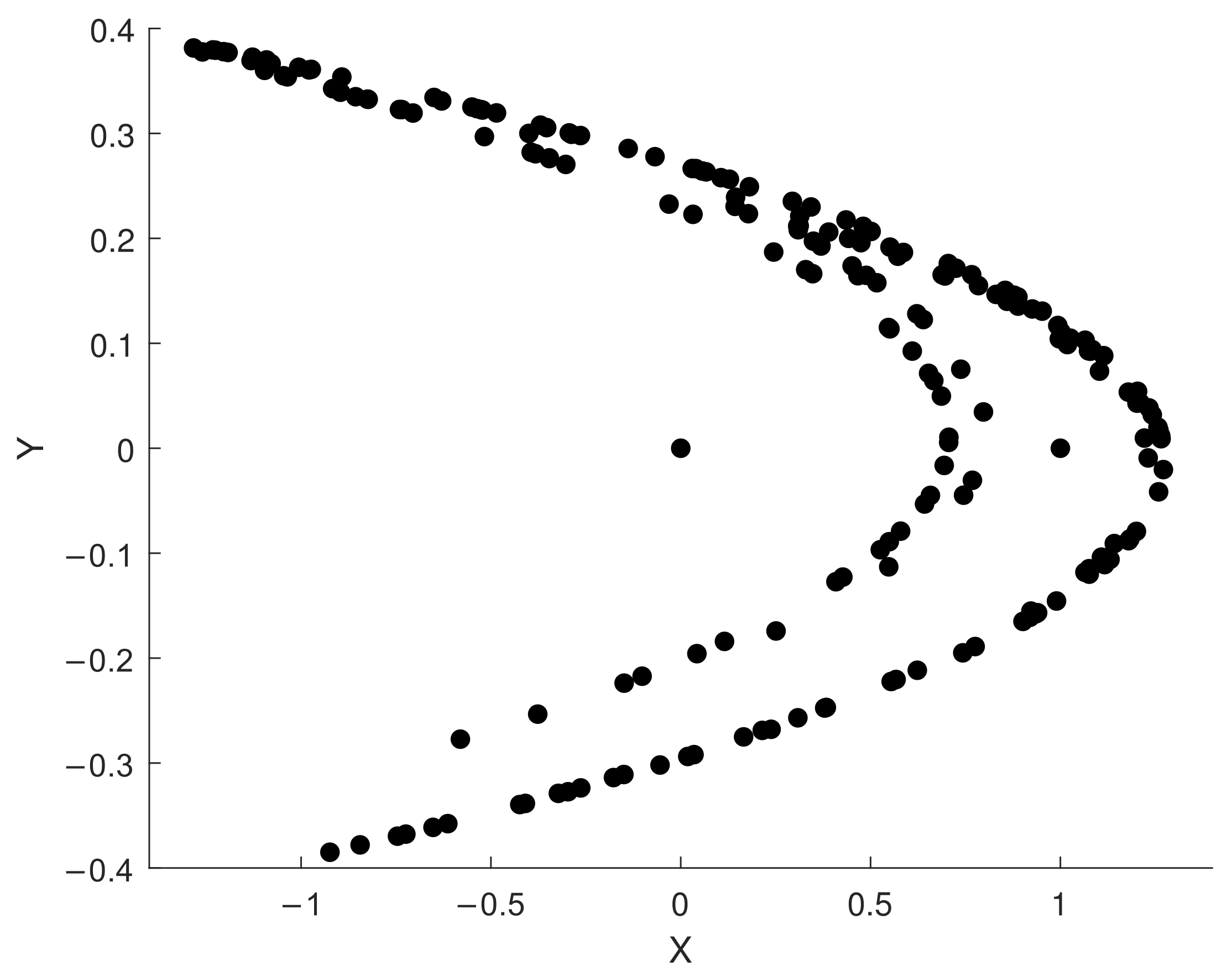
2.1. Chaotic Hénon Map

Hénon’s map is a two-dimensional discrete-time dynamical system, represented by the following state equations [13]:

$$\begin{array}{cc}\hfill x_h(n+1)& =1-a{x}_h^2\left(n\right)+y_h(n+1),\hfill \\ \hfill y_n(n+1)& =b{x}_h\left(n\right).\hfill \end{array}$$

(1)

This map depends on a and b parameters, whose classical values for chaos generation are $a=1.4$ and $b=0.3$. For other a and b values, this map can be intermittent and converge to a periodic orbit or a fixed point. Figure 2 shows the chaotic attractor generated by Hénon’s map by initial conditions $x_h\left(0\right)=y_h\left(0\right)=0$.

2.2. Fractal Dimension

The Oxford dictionary [14] defines fractals as “A curve or geometrical figure, each part of which has the same statistical character as the whole”. They are useful in modeling structures (such as snowflakes) in which similar patterns recur at progressively smaller scales, and in describing partly random or chaotic phenomena such as crystal growth and galaxy formation. The so-called fractal objects are very complex and detailed. If we amplify one section of such object, we find such complexity and detail as the whole object, so smaller sections are similar to the largest ones [15].

A definition of fractal dimension is that of similarity, also called self-similarity, suggested by Felix Hausdorff in 1919, later readjusted by Besicovich (dimension of Hausdorff–Besicovich) [16]: If N equal entities can be obtained from another entity H, similar to the original, with a similarity reason l, then the topological dimension of H is the real number D that verifies,

$$N+l^D=1.$$

(2)

Meaning   

$$D=\frac{logN}{log1/l}.$$

(3)

There are certain geometric objects for which the D dimension is not an integer. We will call such geometric objects, using Benoit Mandelbrot terminology, fractals. In this work we use the mentioned dimension D to corroborate the presence of chaos in the generated trajectories for mobile robots.

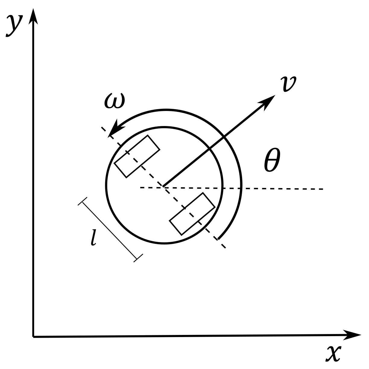
3. Mathematical Model of a Differential Drive Mobile Robot

The behavior of a differential drive mobile robot is based on two independent wheels, one on each side of the robot’s body (Figure 3). Movement is achieved by applying different velocity values to each wheel. This way, the robot can move forward by making both wheels spin at the same speed, or it can turn in any direction using different speeds for each wheel. In this work, the approximated mathematical model of the differential drive mobile robot is used. Suster-Jadlosvska in [17] presents the following mathematical model for a differential drive mobile robot, observing the following considerations:

• The robot moves in a perfectly flat surface without sliding, despite wheel resistance;
• Robot position is given by x, y, and $\theta$ coordinates, where $\theta$ represents the robot rotation in relation to the coordinate system.

The position and rotation of the robot in the plane are based on the following state equations, forming the kinematic model of the mobile robot [17]:

$$\begin{array}{cc}\hfill \dot{x}& =vcos\left(\theta \right),\hfill \\ \hfill \dot{y}& =vsin\left(\theta \right),\hfill \\ \hfill \dot{\theta }& =\omega .\hfill \end{array}$$

(4)

with v and $\omega$ defined as follows:

$$\begin{array}{c}v=\frac{v_l+v_r}{2},\\ \omega =\frac{v_r-v_l}{l}.\end{array}$$

(5)

where v is linear speed, $\omega$ is the angular speed, $\theta$ is the robot’s orientation angle, l the distance between wheels, $v_r$ is the right wheel speed, $v_l$ the left wheel speed, and $l=8.841$ cm (for simulation purposes, this value was taken from the distance between the two wheels present in the Khepera III mobile robot, presented in Section 7.1). A graphic representation of these variables is shown in Figure 3.

Isolating $v_l$ y $v_r$ from Equation (5) we obtain:   

$$\begin{array}{cc}\hfill & v_l=v-(l\ast \omega ),\hfill \\ \hfill & v_r=v+(l\ast \omega ).\hfill \end{array}$$

(6)

These Equations (6) will be used later for the numerical simulations.

The goal of this work is to generate chaotic behavior in the linear v and angular $\omega$ speed of the differential drive robot, described by Equations (4) and (5). To make this possible, an algorithm is designed using the Hénon map (1) as described in the sequel.

4. Proposed Chaotic Trajectory Generator Algorithm for a Differential Drive Mobile Robot

The following algorithm is used for numerical simulations and generation of chaotic trajectories in a differential drive mobile robot. The equations corresponding to every stage are shown in Algorithm 1. The block diagram of the proposed algorithm is shown in Figure 4.

In step 1, the initial positions ($x_0,y_0$) of the differential drive robot are taken as initial conditions for the Hénon map (Equation (1)). In step 2, the current values of Hénon’s chaotic map are calculated ($x_h(n+1),y_h(n+1)$) and then assigned to the linear and angular speeds ($v\left(n\right)$ and $\omega \left(n\right)$) in step 3. Next, in step 4, right and left wheel speeds ($v_l$ and $v_r$) are calculated, obtaining the histograms shown in Figure 5. Then, a homogeneous dispersion is applied to these values in step 5, allowing us to re-scale the maximum and minimum speed values ($v_{dl}$, $v_{dr}$) to the ones used by an actual differential drive mobile robot. Lastly, $v_{dl}$ and $v_{dr}$ values are sent to the mobile robot, which will be used for movement for 2 s (step 6). This execution time was chosen to allow the mobile robot to move in the work area.

Algorithm 1. Proposed Algorithm

Input:$(x_0,y_0)=$ Initial position $(x,y)$ of the robot in the work area, $steps=$ iterations

Output:$v_{dl}$, $v_{dr}=$ Left and right speeds for the mobile robot wheels

1: $x_h\left(0\right)=x_0/1000$,

$y_h\left(0\right)=y_0/1000$,

n = 0;

While $1\le n\le steps$do

2: $x_h(n+1)=1-a{x}_h^2\left(n\right)+y_h\left(n\right)$

$y_h(n+1)=b{x}_h\left(n\right)$;

3: $v\left(n\right)=x_h(n+1)$

$\omega \left(n\right)=y_h(n+1))$;

4: $v_l=v\left(n\right)-l\omega \left(n\right)$

$v_r=v\left(n\right)+l\omega \left(n\right)$;

5: $v_{dl}=floor((\left(100v_l\right)-floor\left(100v_l\right))\ast 180)+20$

$v_{dr}=floor((\left(100v_r\right)-floor\left(100v_r\right))\ast 180)+20$;

6: $t=2$ s;

7: $n=n+1$.

end

return $v_{dl}$, $v_{dr}$

The number of iterations is determined by the application, each with an execution time of two seconds. For example, if the robot is required to operate for 2 min (that is, 120 s), the desired number of iterations would be 60. The number of iterations could be related to another kind of application; for example, the algorithm could stop when an object is found or a certain coverage percentage is achieved.

Isolating left and right wheel speeds from Equation (5), we obtain the histograms shown in Figure 5. We can observe that $v_l$ and $v_r$ values are mostly negative and positive, respectively, indicating that the resulting trajectory will be primarily based on left turns. Very similar behavior can be observed with different numbers of iterations. Because of this, dispersion and uniformity measures need to be taken for $v_l$ and $v_r$ values, as shown in Figure 6. The dispersion allows performing a re-escalation of the values to a range of velocities usable by the robot, limiting the minimum and maximum values so that the robot can use them without any problem.

This speed range does not include negative values, preventing the robot from moving in reverse, so that the generated trajectory encompasses a larger area of coverage in a shorter time. The two-second run time in step 6 in Algorithm 1 is used to allow the robot to have the opportunity to move properly and to have greater coverage of the work area. This run time can be adjusted according to the individual capacities of the mobile robot type to implement (maximum and minimum speed, movement type, etc.). To perform the numerical simulations, an HP laptop with an A10 processor of 1.9 GHz, 12 GB of RAM, Windows 10 (64 bit), and MATLAB R2019a were used.

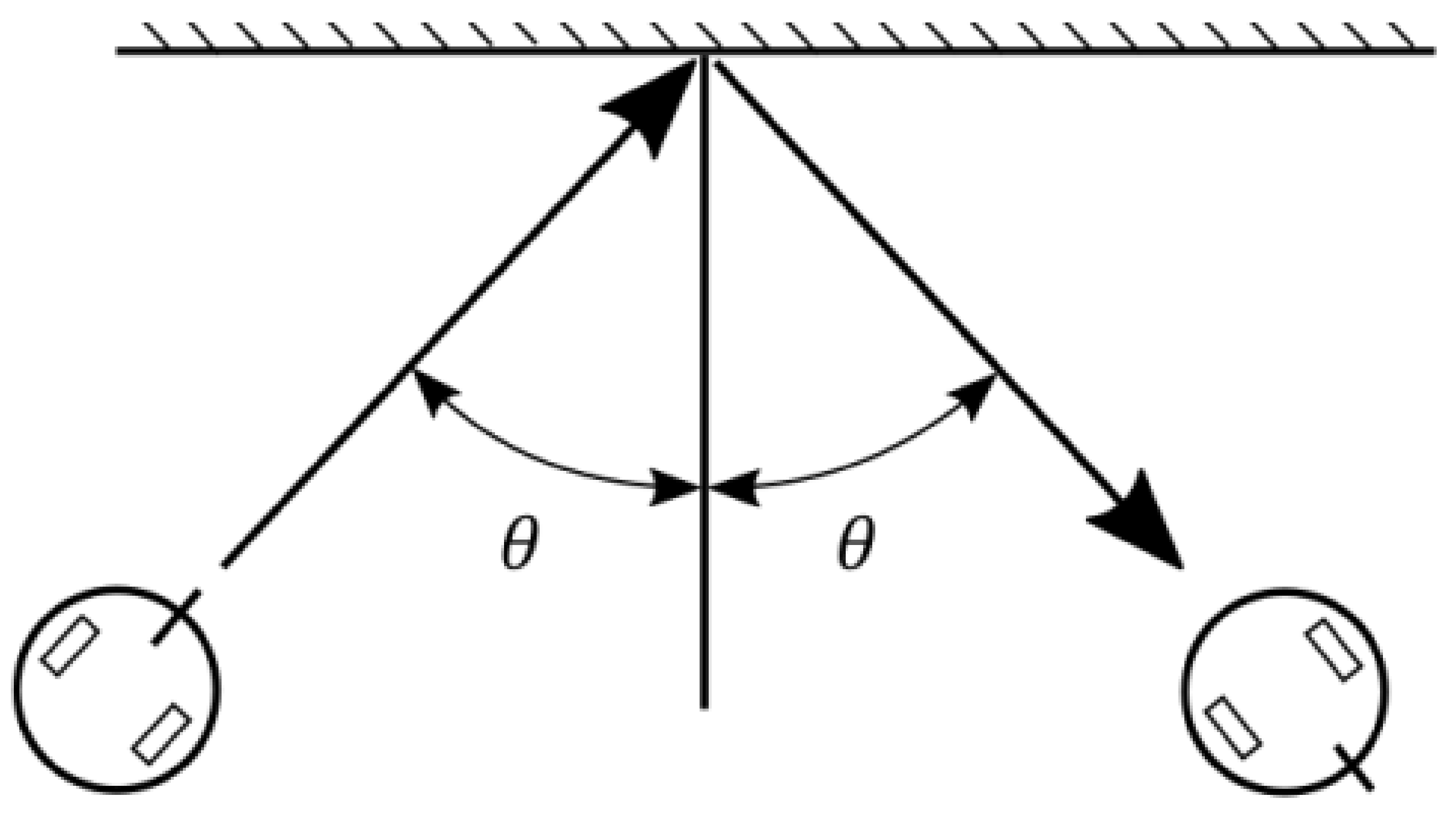
Work Area Boundaries

The work area size is 1400 × 2400 mm. The control objective is that the differential drive mobile robot covers the largest possible area of the work space in a chaotic way. The robot must change its trajectory when it reaches some of the boundaries of the work area to avoid colliding with them. In this case, a reflexive movement is adopted. When the robot senses proximity to one of these limits, the robot changes its direction of movement following the strategy shown in Figure 7. It takes an exit path at an angle that reflects the entry angle.

5. Results

In this section, the obtained results from the numerical simulations are reported. Starting the trajectory of the robot at the origin $(x,y,\theta )=(0,0,0)$, numerical simulations were carried out based on the proposed chaos generator algorithm with 200 and 300 iterations. The obtained results can be seen in Figure 8. The inner rectangle represents the boundaries of the work area previously described. Each color represents a time lapse of two seconds during which the mobile robot uses the speed values obtained from the proposed algorithm (that is, for each iteration) before moving on to the next speed values.

Figure 8 shows that the trajectories of the robot are apparently unpredictable and, with 300 iterations, the differential drive mobile robot covers (patrols) most of the work area. It is important to mention that, in the numerical simulations, the real dimensions of the robot are not considered, so the area actually covered by the robot is much larger than the one shown in the graphs. It can also be observed from these results (Figure 8), that the followed trajectory is the same in all cases under the same initial conditions, confirming the deterministic nature of the chaos. However, simulations to obtain Figure 9 were carried out using two different initial positions (in millimeters) with the same orientation $({\theta }_0=0)$$(x_0,y_0)=(0,0.01)$ in Figure 9a, and $(x_0,y_0)=(-350,500)$ in Figure 9b. For each case, 200 iterations of the designed algorithm were performed to compare the generated trajectories.

Comparing Figure 8a and Figure 9a, it can be observed that trajectories change drastically despite having a change of only 0.01 mm in the initial condition of the x-axis, demonstrating sensitivity to initial conditions typical of a chaotic system.

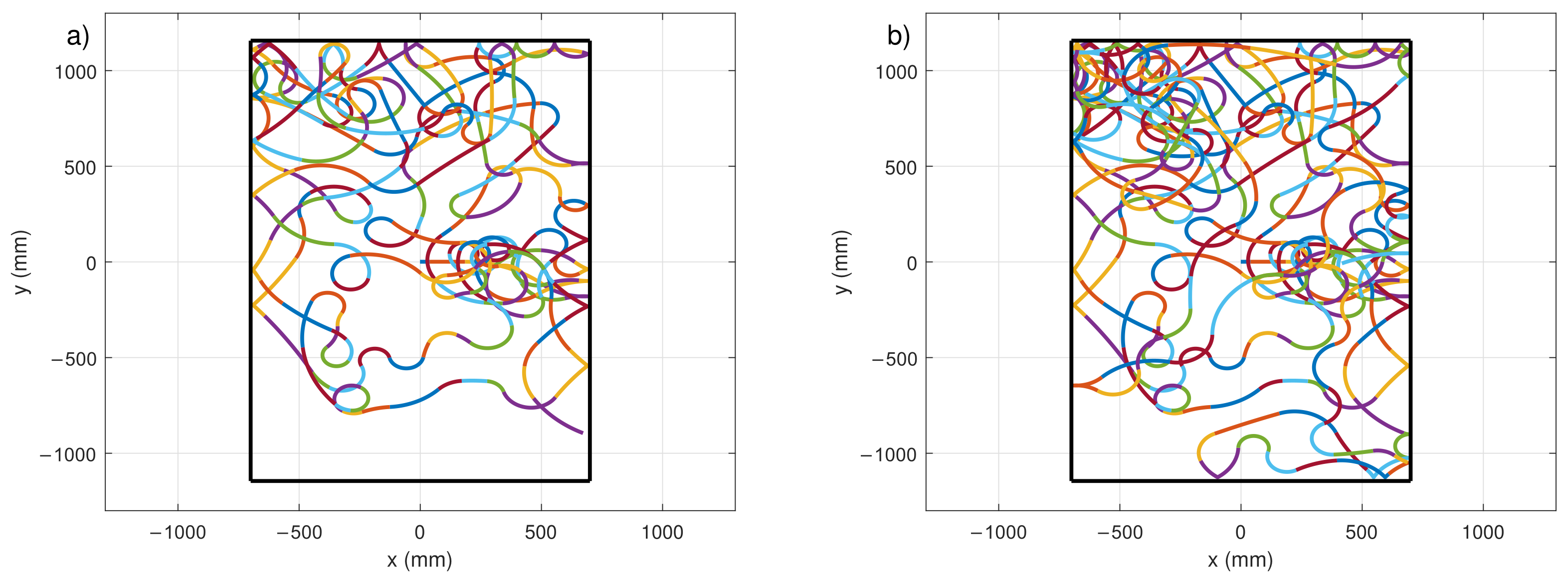
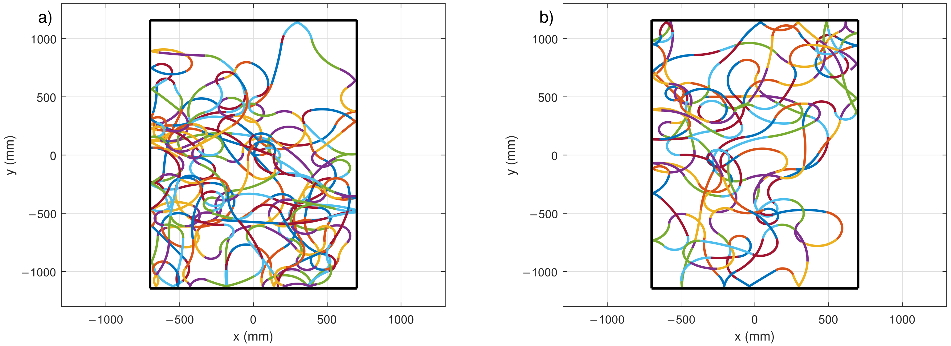
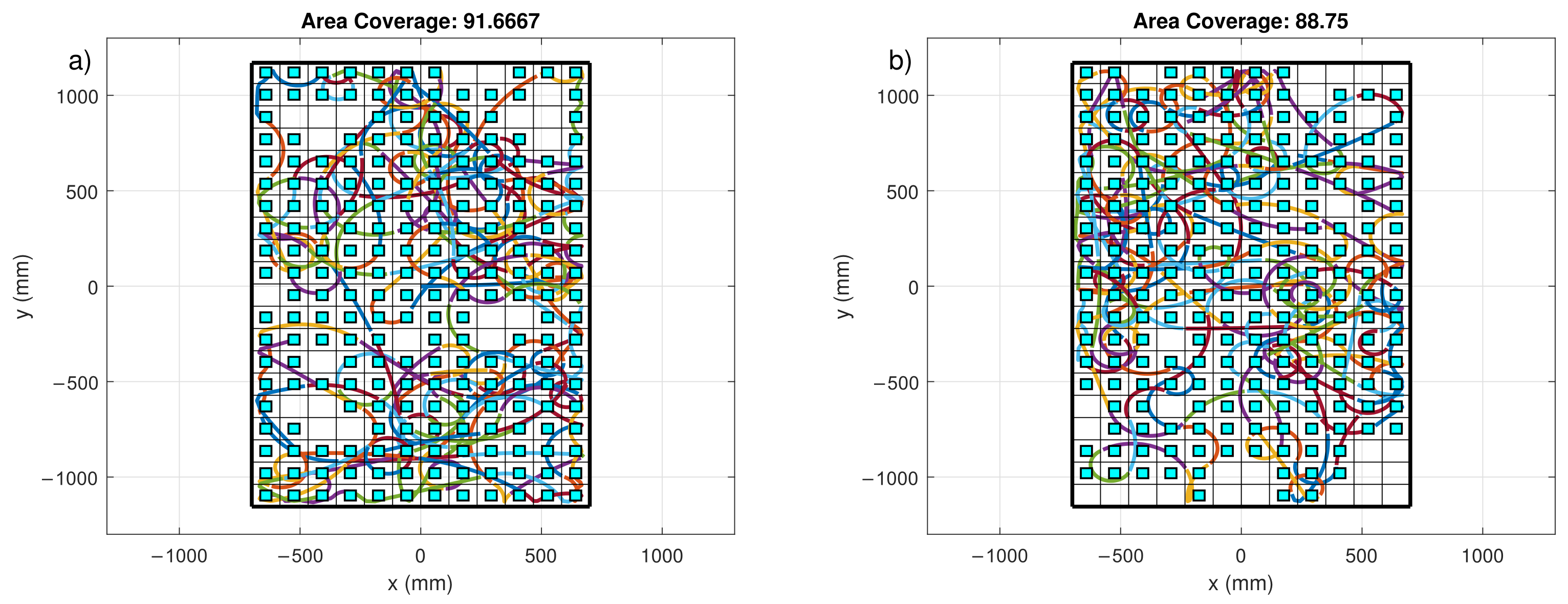
5.1. Coverage of the Work Area

In order to estimate the work area covered by the chaotic trajectories imposed by Algorithm 1 on the mobile robot, it was divided into a grid of 12 × 20 $\left(240\right)$ frames with lateral measurements of 76.66 mm; this is to have a more precise idea of the effective coverage of the differential drive mobile robot employing the proposed algorithm for exploration or search applications. Figure 10 shows the percentage coverage of the test area by the differential drive mobile robot for 100 and 300 iterations of the trajectories imposed by Algorithm 1, when the initial conditions were $(x_0,y_0,{\theta }_0)=(0,0,0)$. We can see that with just 100 iterations the robot patrolled almost half of the work area and with 300 iterations it covered almost the entire work surface.

Repeating the previous process 1000 times for arbitrarily selected initial conditions, using 300 iterations, an average of $84.1270\%$ of covered work area is obtained.

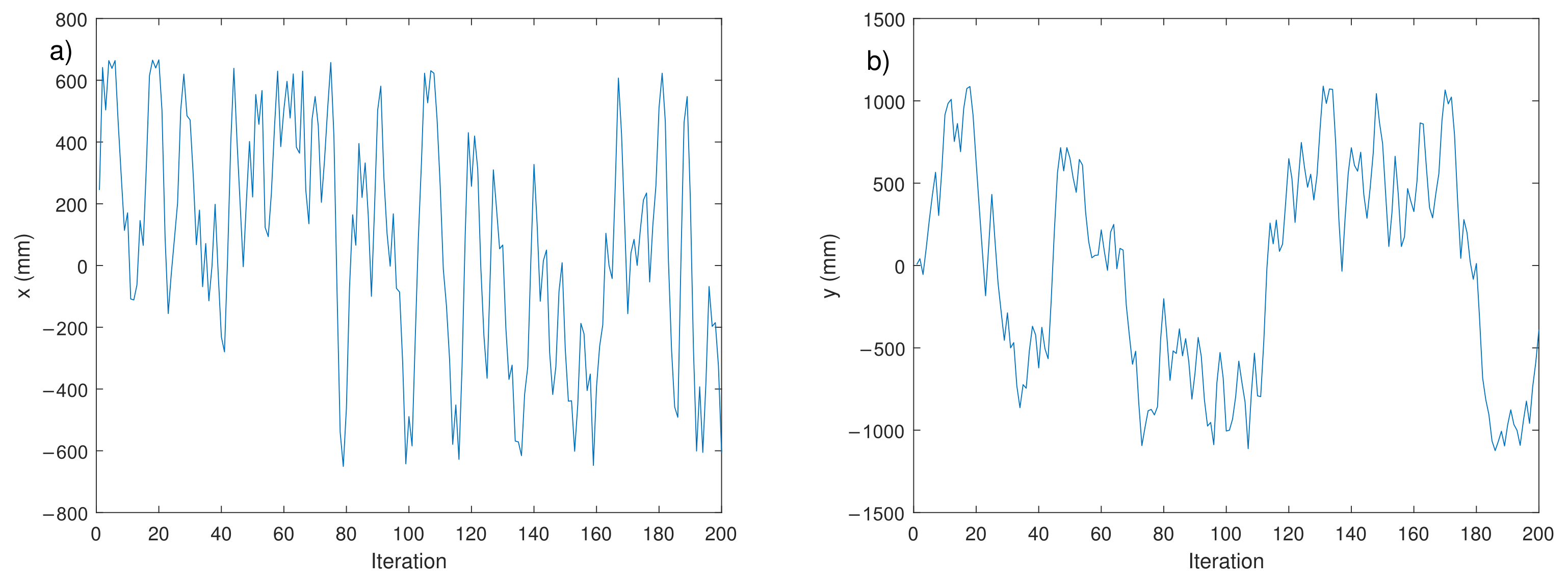
5.2. Gottwald–Melbourne Test

To verify that the trajectories generated by the proposed algorithm are indeed chaotic, we use the 0-1 Gottwald–Melbourne test [18]. This test determines if a discrete deterministic dynamic system is chaotic or not. Contrary to the usual method of calculating the maximum Lyapunov exponent, this method is applied directly to the time series and does not require space-phase reconstruction. In addition, the dimension of the dynamic system and the form of its equations are irrelevant. To perform the test, 300 iterations of the chaotic trajectory generator algorithm are executed to the mobile robot with different initial conditions. Taking into consideration the data of the time series of the x and y states of the model of the differential drive mobile robot, obtained from the results of the performed numerical simulations, we can perform the 0-1 test to verify evidence of chaos in the trajectories of the mobile robot generated by the algorithm. The input is the data of the time series and the output is the amount of chaos between 0 and 1; this value indicates whether the input is chaotic or not, 0 denoting not chaotic and 1 totally chaotic. The test is applied to any dynamic deterministic system; see details of the test in [18]. Figure 11 shows the time series of the x and y coordinates for the initial experimental conditions $(x_0,y_0,{\theta }_0)=(0,0,0)$.

The resulting value of the 0-1 test for our proposed algorithm in the x axis is $0.9854$ and for the y axis is $0.9745$. The number close to 1 is a clear indication that the test concludes that such time series are indeed chaotic.

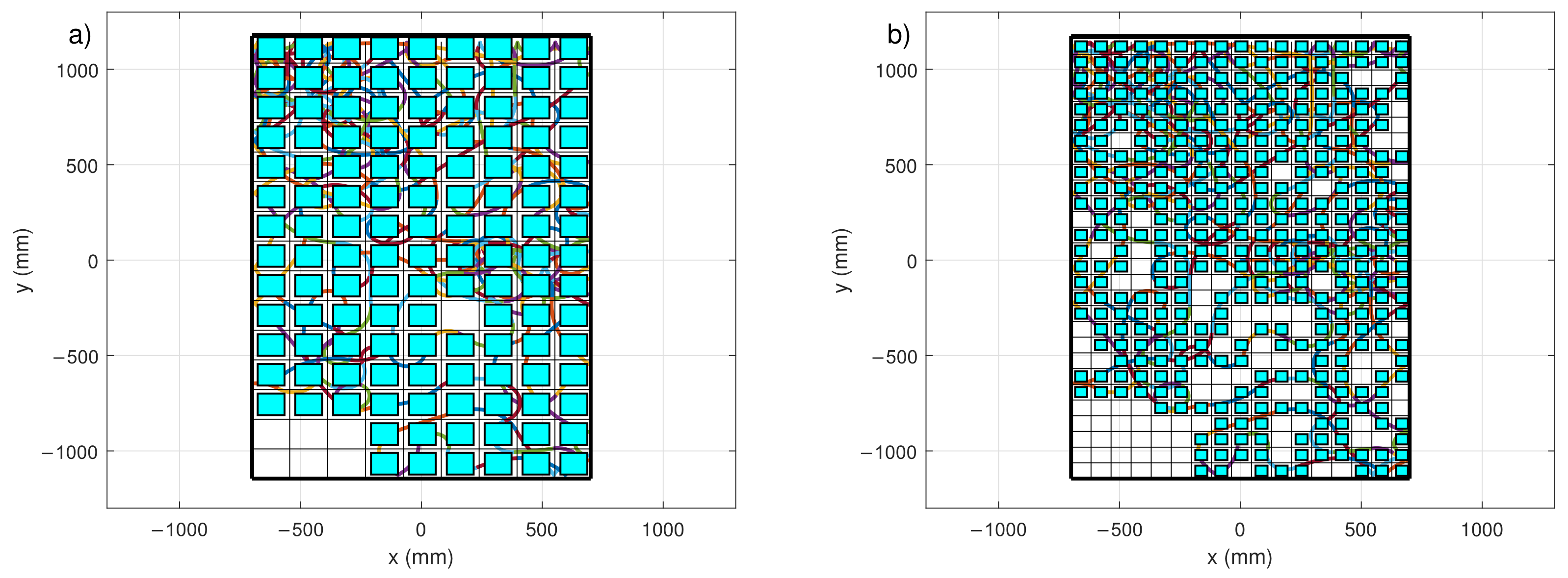
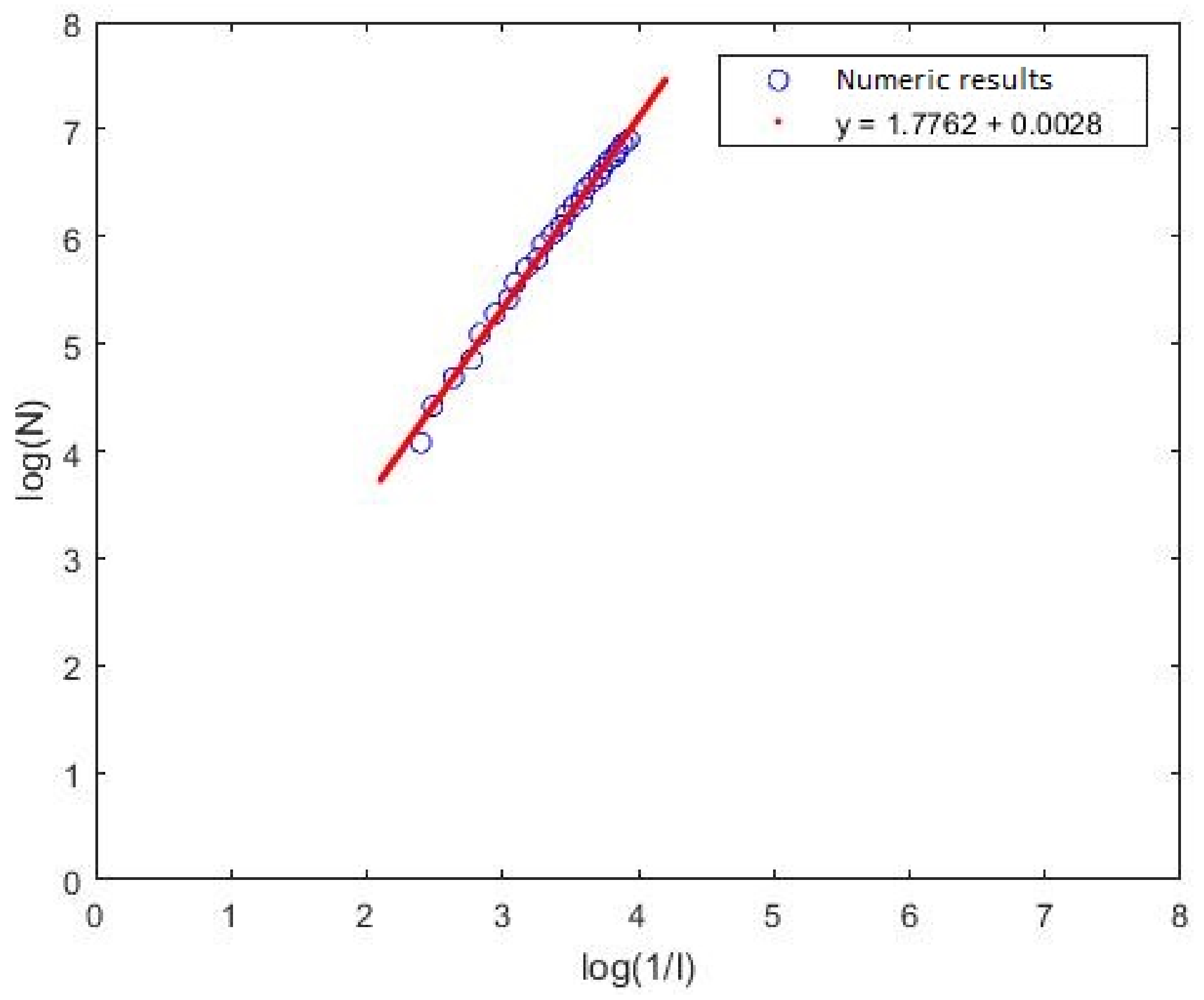
5.3. Box-Counting Test

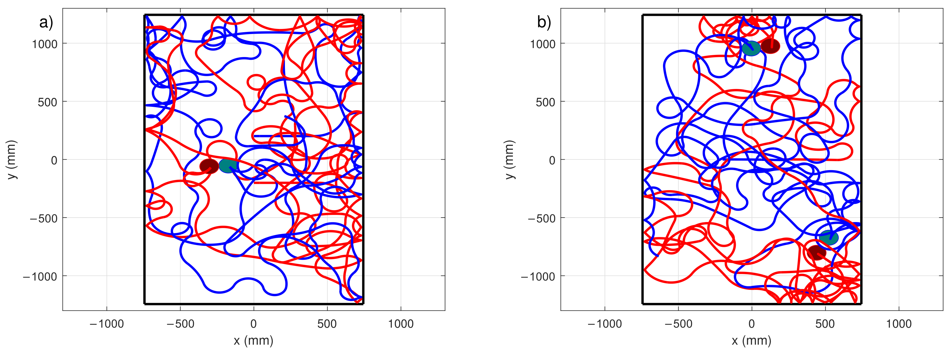
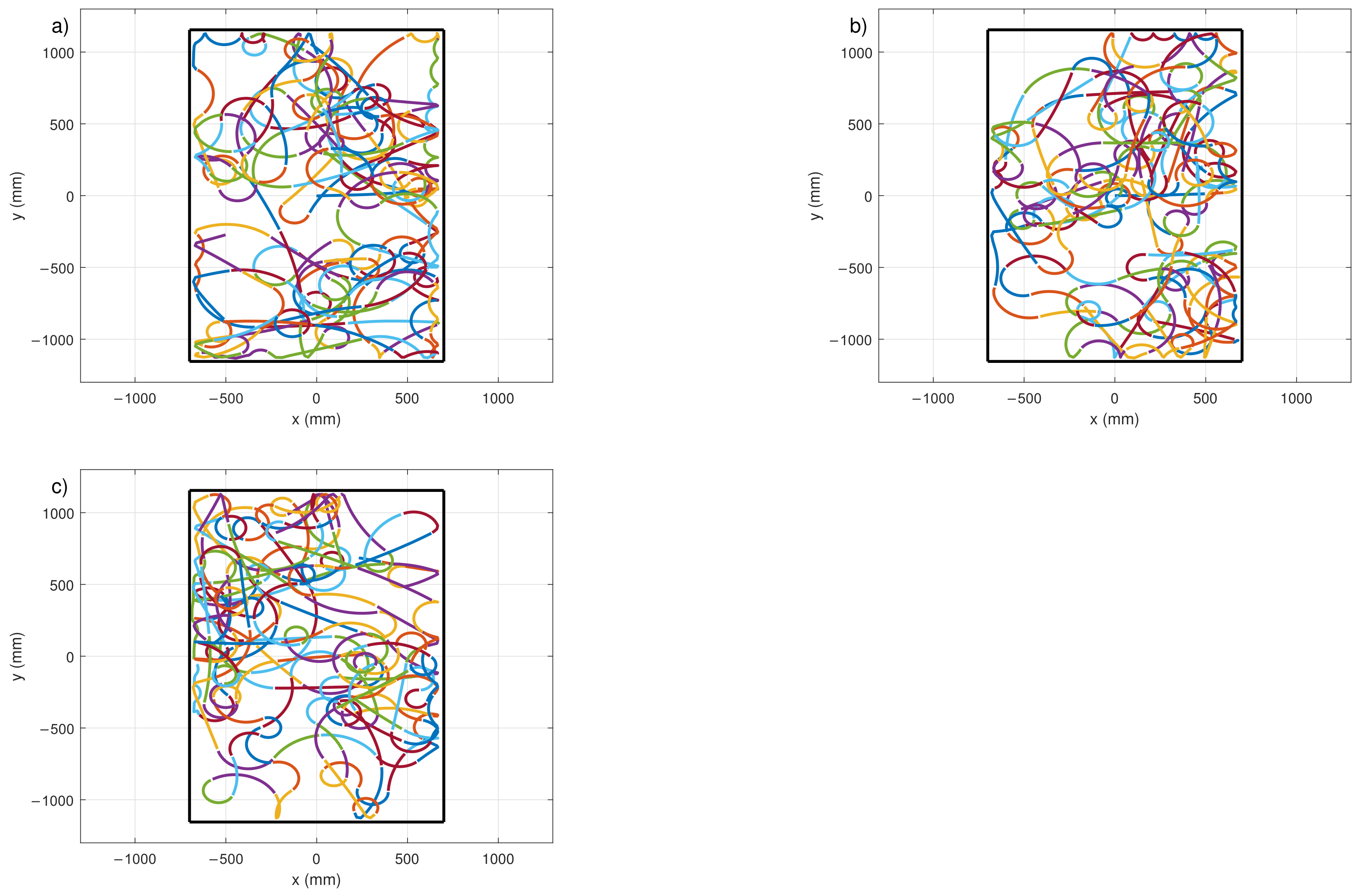
Some techniques used to estimate the fractional dimension of a geometric object were discussed by Mandelbrot [19]. In this work, the box-counting method is applied because of its simplicity, automatically calculable with the use of computer and applicable for patterns with or without self-similarity. In this test, each image or geometric object is covered by a sequence of squares of descendant measurements and for each of the squares two values are stored: the number of boxes intersected by the image $N\left(l\right)$ and the lateral length of each frame l. The regression slope D of the straight line formed by the plot of $logN\left(l\right)$ against $log1/l$ indicates the degree of complexity (or fractional dimension) between 1 and 2; $1\le D\le 2$ [19]. An image with a fractional dimension of 1 or 2 is considered completely differentiable. The linear regression used to estimate the fractional dimension [20] is given by

$$logN\left(l\right)=logK+Dlog1/l,$$

(7)

where K is a constant and $N\left(l\right)$ is proportional to ${(1/l)}^{-D}$. Clearing D from Equation (7) we obtain the following expression:

$$D=\frac{logN}{log1/l}.$$

(8)

To perform this test, we return to the grid used to measure the percentage of coverage of the test area performed by the trajectories of the mobile robot generated by the algorithm designed in this work. The size of the grid with $l=1$ will be taken for the case when the length of the work area (the dimensions of the work area are 1400 × 2400 mm) is equal to the length of a grid square. We start with squares of size $l=0.111$, which will be reduced until we obtain very small squares (boxes) of size $l=0.0200$. We take the path of the robot generated with the initial conditions $(x_0,y_0,{\theta }_0)=(0,0,0)$. Figure 12 shows two different grid sizes for the proposed work area: (a) 135 boxes of $l=0.0667$ and (b) 476 boxes of $l=0.0357$.

After making 25 reductions of the grid and plotting $logN\left(l\right)$ against $log1/l$, the linear regression of the data results in Figure 13. We can see behavior very similar to the line given by the equation $y=1.7762x+0.0028$. Using Equation (8) for every grid size reduction we obtain $D=1.7762$, which is a fractional dimension and therefore the trajectories are chaotic.

6. Multiple Robots

In this section, we analyze the behavior obtained when Algorithm 1 is applied to multiple mobile robots. In the next subsections, we show the results obtained for 2, 3, and n robots moving simultaneously in the work area.

6.1. Two Mobile Robots in the Same Work Area

Figure 14 shows the trajectories generated by two differential mobile robots in the same work area with different initial conditions. In this case, when the two robots are close to colliding, a reflective strategy is taken, so that both mobile robots can continue on their way but in the opposite direction (taking a ${180}^{\circ }$ turn). Red and blue circles indicate a collision that is avoided using the reflective strategy. Each simulation is performed with 150 iterations of the proposed algorithm. In both cases, $({\theta }_0=0^{\circ })$ is considered. The blue line represents the trajectory of robot 1 and the red line represents robot 2.

Repeating the procedure (Figure 14) 1000 times with different initial conditions, a coverage percentage average of $83.6429\%$ is obtained. It is important to note that only half of the iterations are necessary to cover a percentage of the work area similar to the case when using a single mobile robot.

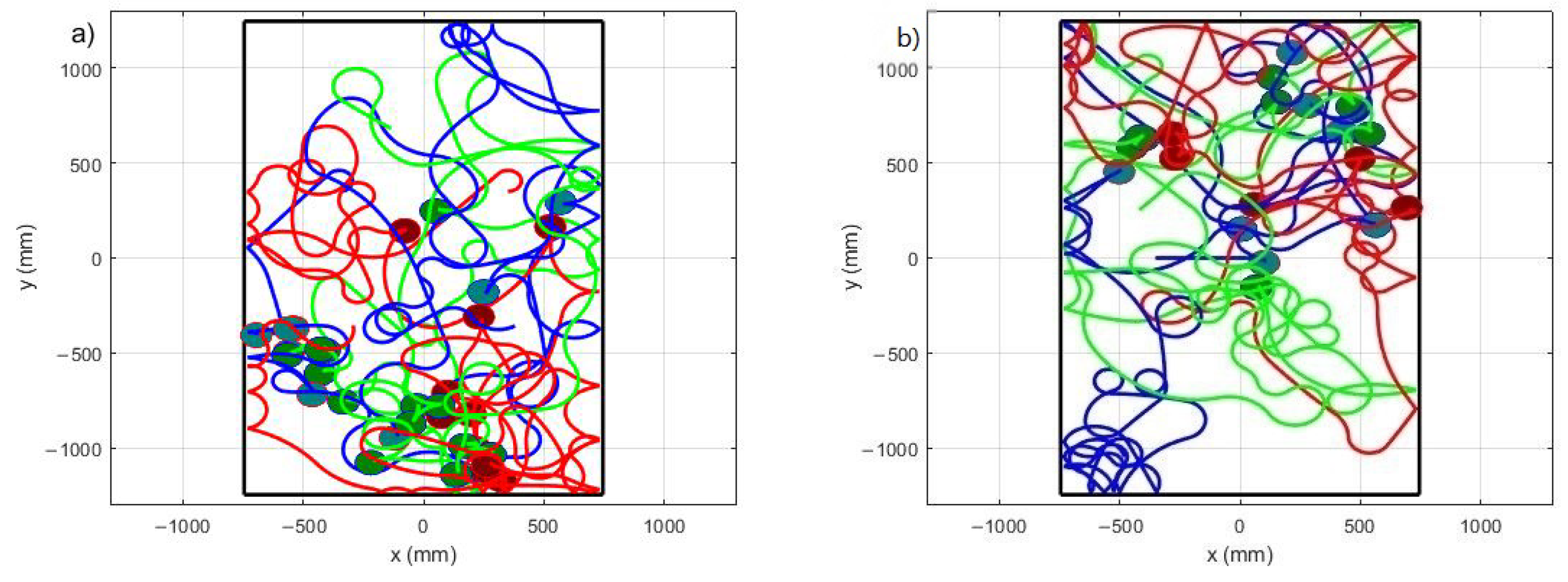
6.2. Three Mobile Robots in the Same Work Area

Figure 14 shows the trajectories generated by three differential mobile robots moving simultaneously in the same work area with different initial conditions for each one. In a similar manner to that explained in the previous section, when two or three of the robots are to collide, the reflective strategy is taken. In Figure 15, the red, green, and blue circles indicate a collision that is avoided using the reflective strategy. Each simulation is performed with 100 iterations of the algorithm. The blue line represents the trajectory of robot 1, the red line represents robot 2, and the green line represents the trajectory of robot 3. Repeating the procedure 1000 times with different initial conditions, a coverage percentage average of $84.1826\%$ is obtained. We can see that fewer iterations are needed to cover a percentage of the work area similar to the case when using a single mobile robot.

6.3. n-Mobile Robots in the Same Work Area

In a similar way as before, we repeat the process for n mobile robots $(n\le 10)$. No figure is shown because the trajectories would not be easily visualized due to the number of robots. However, in the next subsection we offer the results obtained for this case.

6.4. Presence of Chaos in Generated Trajectories for Multiple Mobile Robots

Following the procedure shown previously in Section 5, coverage and presence of chaos are analyzed for multiple mobile robots.

6.4.1. Coverage Percentage of the Test Area

In

Table 1. Average coverage percentage for n robots simultaneously in the same work area.

Number of Robots	Coverage (%)
1	18.1250
2	33.7500
3	46.4583
4	55.8333
5	63.3333
6	70.2083
7	75.8333
8	79.3750
9	82.0833
10	85.8300

we show the average coverage percentage obtained for $1\le n\le 10$ mobile robots. The trajectories were calculated using 100 different initial conditions for each robot. We used 25 iterations of the algorithm for each trajectory so the full coverage ($100\%$) was not reached.

It can be observed that the increment in coverage does not follow linear behavior. This is partially due the size of the robot taking up space in the work area, and could also imply that there is an optimum number of robots for a given work area. We plan to further investigate this result as part of our future work.

6.4.2. Gottwald–Melbourne Test

We applied the Gottwald–Melbourne test to verify the presence of chaos in the generated trajectories. We used 300 iterations and different initial conditions for each trajectory.

Table 2. Gottwald–Melbourne results for 10 robots simultaneously in the same work area.

Number of Robots	Result for x	Result for y
1	0.9837	0.9254
2	0.9461	0.9107
3	0.9540	0.9307
4	0.9863	0.9633
5	0.9554	0.9417
6	0.9899	0.9601
7	0.9919	0.9645
8	0.9621	0.9774
9	0.9619	0.9445
10	0.9769	0.9552

shows the average results for x and y after 100 repetitions, and each one is an average of the results of the number of mobile robots used in each case.

For example, in the case of using three robots, the value shown for the x axis is an average of the test result for the three robots, 100 times. We can conclude that, for $1\le n\le 10$ mobile robots moving simultaneously in the work area, chaos is present in their trajectories.

6.4.3. Box-Counting Test

After applying the box-counting test (see Section 5.3) to $1\le n\le 10$ mobile robots, the results shown in

Table 3. Box-counting results for n robots simultaneously in the same work area.

Number of Robots	D
1	1.7762
2	1.7863
3	1.7634
4	1.7787
5	1.7723
6	1.7636
7	1.7864
8	1.7741
9	1.7679
10	1.7769

were obtained.

We can observe that a fractal dimension is present in the generated trajectories even with multiple mobile robots, which is a chaotic property. Based on the obtained result of the tests applied, we can conclude that every generated trajectory by means of the proposed algorithm presented in this work is chaotic.

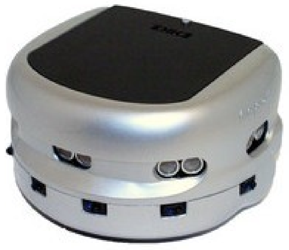
7. Experimental Results

In this section we present the results obtained by applying the proposed algorithm (Algorithm 1) to a real differential drive mobile robot.

7.1. Materials

For the experimental application of the proposed algorithm, a Khepera III differential drive mobile robot (Figure 16) was used. It is a small, circular robot with a diameter of approximately 130 mm, a height of 70 mm and a weight of 650 g. It has two wheels separated by $l=8.841$ cm and a sliding stand. It has a speed range of $(-200$ to $-20)$ and $(20$ to $200)$ mm/s.

Eight Flex 13 cameras and the Motive software, by Optitrack, were used for robot position measuring. This setup uses infrared lights, allowing real-time position measuring of small reflective spheres placed on top of the Khepera III robot with a precision of tens of millimeters. The software can export real live data, easily retrievable by Matlab. This allows the generation of the same type of graphical representation as the ones presented for the simulations in Section 5, enabling an easier visual comparison between the numerical and experimental results.

7.2. Methodology

Three experiments with the Khepera III differential robot were performed using different initial conditions with 200 iterations for each of the following cases:

• $x_0=1.1$, $y_0=-0.9$, ${\theta }_0=1.8^{\circ }$;
• $x_0=-0.5$, $y_0=-1.3$, ${\theta }_0=359.1^{\circ }$;
• $x_0=232.1$, $y_0=685.3$, ${\theta }_0=-10.3^{\circ }$.

The black square represents the boundaries of the work area (table) described above. The dimensions of the table are 1400 × 2400 mm, the same as the work area taken for the simulations shown in previous sections.

The experimental results are shown in Figure 17. Each color represents a time span of two seconds during which the robot uses the speed values obtained by each iteration before moving to the next ones.

It can be seen from Figure 17a,b that a small change in millimeters in the initial conditions produces completely different and unpredictable trajectories in the robot, demonstrating experimentally that the chaotic property of sensitivity to initial conditions is met. It is notable that with 200 iterations most of the work area is covered. It should be mentioned that these experimental results are preliminary; it is necessary to improve the algorithm of evasion of edges so that the angle of reflection is more precise and use other chaotic systems to compare their performance.

7.3. Coverage of the Work Area

In order to estimate the work area covered by the chaotic trajectories imposed on the mobile robot, it was divided into a grid of 12 × 20 $\left(240\right)$ frames with lateral measurements of 76.66 mm, so we can have a more precise idea of the effective coverage of the proposed Algorithm 1 for exploration or search applications. In Figure 18 the results obtained from the trajectory of the Khepera III robot with initial conditions $x_0=1.1$, $y_0=-0.9$, $\theta =1.8^{\circ }$ and $x_0=232.1$, $y=685.3$, $\theta =-10.3^{\circ }$ are shown.

We can see that, with only 200 iterations of the chaotic trajectory generator algorithm, the test area is covered almost entirely. It should be remembered that the area occupied by the robot and the range of its sensors are not taken into account.

7.4. Gottwald–Melbourne Test

Figure 19 shows the time series of the x and y coordinates for the initial experimental conditions $x_0=1.1$, $y_0=-0.9$, ${\theta }_0=1.8^{\circ }$.

The resulting value of the test for x is 0.9743 and for y is 0.9465. The number close to 1 is a clear indication that the test concludes that such time series are indeed chaotic.

7.5. Box-Counting Test

We took the path of the robot generated with the initial conditions $x_0=1.1$, $y_0=-0.9$, ${\theta }_0=1.8^{\circ }$ for this test.

Table 4. Experimental box-counting results for n robots simultaneously in the same work area.

$\mathit{N}\left(\mathit{l}\right)$	l	$log\mathit{N}\left(\mathit{l}\right)$	$log1/\mathit{l}$	D
59	0.0909	4.0775	2.3978	1.7004
108	0.0714	4.6821	2.6391	1.7742
225	0.0476	5.4161	3.0445	1.7789
329	0.0384	5.7960	3.2580	1.7789
447	0.0322	6.1025	3.4339	1.7770
570	0.0277	6.3456	3.5835	1.7707
709	0.0256	6.5638	3.7135	1.7675
848	0.0217	6.7428	3.8286	1.7611
995	0.0196	6.9027	3.9318	1.7556
			$D_{Mean}$	$1.7750$

shows the measured values of N, l, $logN\left(l\right)$, $log1/1$, and D for this case.

When plotting $logN\left(l\right)$ against $log1/1$ and performing the linear regression to the data shown, we obtained Figure 20. We can see behavior very similar to the line given by the equation $y=117837x-0.0462$.

We note that the slope of this line ($1.7762$) is very similar to the obtained values of D. This result verifies that the trajectory has a fractional dimension and, therefore, is chaotic. Among the conditions that affect the experimental results are the intrinsic physical limitations of the Khepera III robot, as well as some characteristics of the test area.

8. Conclusions

In this paper, a simple and easy-to-implement algorithm to generate trajectories infused with chaotic properties was designed, using Hénon’s map to produce wheel speeds for the mobile robot to use. This allows the robot to have unpredictable movement, making it ideal for patrolling purposes. The obtained numerical results confirm that these trajectories are unpredictable. Numerical tests were performed to determine the existence of chaos in the generated trajectories for the differential drive mobile robot. The Gottwald–Melbourne test shows that the resulting time series are indeed chaotic, while the box-counting test shows that the final trajectory has a fractional dimension and, therefore, is chaotic.

Numerical tests also show that, for $1\le n\le 10$ mobile robots running simultaneously, the generated trajectories are still chaotic. Furthermore, experimental results show that applying the proposed algorithm to a real differential drive mobile robot successfully imparts it with chaotic properties.

With these results, the authors of this work believe that we leave a solid base from which to reproduce the results obtained in this work for its application in other research, with applications such as border patrol, dangerous object search (for example, explosives), rescue, and unknown territory exploration, among others.

For future work, the improvement of the edge evasion strategy will be proposed. In addition, other chaotic systems will be implemented to compare the behavior and generated trajectories for different mobile robots. We will work on the verification of the presence of chaos in the generated trajectories of the differential mobile robots using other indicators of chaos. We will also analyze the existence of optimal initial conditions that allow high work area coverage with few iterations for one and multiple mobile robots.

References

1. Li, L.; Penq, H.; Kurths, J.; Yang, Y.; Schellnhuber, H. Chaos—Order transition in foraging behavior of ants. Proc. Natl. Acad. Sci. USA 2014, 111, 8392–8397. [Google Scholar] [CrossRef] [PubMed] [Green Version]
2. Nakamura, Y.; Sekiguchi, A. The Chaotic Mobile Robot. IEEE Trans. Rob. Autom. 2001, 17, 898–904. [Google Scholar] [CrossRef]
3. Martins-Filho, L.; Macau, E. Kinematic control of mobile robots. ABCM Symp. Ser. Mech. 2006, 2, 258–264. [Google Scholar]
4. Volos, C.K.; Kyprianidis, I.M.; Stouboulos, I.N. A chaotic path planning generator for autonomous mobile robots. Robot. Auton. Sys. 2012, 60, 651–656. [Google Scholar] [CrossRef]
5. Curiac, D.; Volosencu, C. A 2D chaotic path planning for mobile robots accomplishing boundary surveillance missions in adversarial conditions. Comm. Nonlin. Sci. Num. Sim. 2014, 19, 3617–3627. [Google Scholar] [CrossRef]
6. Pliego-Jiménez, J.; Martínez-Clark, R.; Cruz-Hernández, C.; Arellano-Delgado, A. Trajectory tracking of wheeled mobile robots using only Cartesian position measurements. Automatica 2021, 133, 109756. [Google Scholar] [CrossRef]
7. Martínez-Clark, R.; Cruz-Hernández, C.; Pliego-Jiménez, J.; Arellano-Delgado, A. Control algorithms for the emergence of self-organized behaviors in swarms of differential-traction wheeled mobile robots. Int. J. Adv. Robot. Syst. 2018, 15, 172988141880643. [Google Scholar] [CrossRef]
8. Montañez-Molina, C.; Pliego-Jiménez, J.; Cruz-Hernández, C. Chaotic velocity profile for surveillance tasks using a quadrotor. In Proceedings of the 2021 IEEE Conference on Control Technology and Applications (CCTA), San Diego, CA, USA, 9–11 August 2021. [Google Scholar]
9. Nasr, S.; Mekki, H.; Bouallegue, K. A multi-scroll chaotic system for a higher coverage path planning of a mobile robot using flatness controller. Chaos Solitons Fractals 2018, 118, 366–375. [Google Scholar] [CrossRef]
10. Majeed, A.I. Mobile Robot Motion Control Based on Chaotic Trajectory Generation. J. Eng. Sustain. Dev. 2010, 24, 26–33. [Google Scholar]
11. Petavratzis, E.K.; Volos, C.K.; Moysis, L.; Stouboulos, I.N.; Nistazakis, H.E.; Tombras, G.S.; Valavanis, K.P. An Inverse Pheromone Approach in a Chaotic Mobile Robot’s Path Planning Based on a Modified Logistic Map. Technologies 2019, 7, 84. [Google Scholar] [CrossRef] [Green Version]
12. Martins-Filho, L.; Luiz, S.; Machado, R.F.; Rocha, R.; Vale, V.S. Commanding mobile robots with chaos. In Proceedings of the ABCM Symposium Series in Mechatronics, Sao Paulo, SP, Brazil, 10–14 November 2004; Volume 1. [Google Scholar]
13. Hénon, M. A Two-Dimensional Mapping with a Strange Atractor. Comm. Math. Phys. 1976, 50, 69–77. [Google Scholar] [CrossRef]
14. Dictionary, Oxford English. In Oxford Dictionary of English, 3rd ed.; Oxford University Press: Oxford, UK, 2010; ISBN 0199571120.
15. Torres, N. Caos en sistemas biológicos. Mat. Rev. Dig. Div. Mat. Real Soc. Mat. Esp. 2005, 1, 478–482. [Google Scholar]
16. Besicovitch, A. On linear sets of points of fractional dimension. Math. Ann. 1929, 101, 161–193. [Google Scholar] [CrossRef]
17. Suster, P.; Jadlovska, A. A Neural tracking trajectory of the mobile robot Khepera II internal model control structure. In Proceedings of the International Conference Process, Kouty nad Desnou, Czech Republic, Prague, 7–10 June 2010. [Google Scholar]
18. Gottwald, G.A.; Melbourne, I. A new test for chaos in deterministic systems. Proc. R. Soc. Lond. A Math. Phys. Eng. Sci. R. Soc. 2004, 460, 603–611. [Google Scholar] [CrossRef] [Green Version]
19. Mandelbrot, B.B. The Fractal Geometry of Nature; WH Freeman: New York, NY, USA, 1983; Volume 1, p. 173. [Google Scholar]
20. Macmillan, K.; Foroutan-Pour, P.; Dutilleul; Smith, D. Advances in the implementation of the box-counting method of fractal dimension estimation. Appl. Math. Comp. 1999, 105, 195–210. [Google Scholar]
Figure 1. Predictable vs. unpredictable trajectories: (a) predictable; (b) unpredictable.
Applsci 12 02587 g001
Figure 2. Hénon’s map chaotic attractor.
Applsci 12 02587 g002
Figure 3. Graphic representation of the differential drive mobile robot model.
Applsci 12 02587 g003
Figure 4. Block diagram of the proposed chaotic trajectory generator Algorithm 1.
Applsci 12 02587 g004
Figure 5. Wheel speed histograms: (a) left speed v l ; (b) right speed v r .
Applsci 12 02587 g005
Figure 6. Wheel speed histograms after dispersion in step 5: (a) dispersed left speeds v d l ; (b) dispersed right speeds v d r .
Applsci 12 02587 g006
Figure 7. Reflective edge avoidance strategy.
Applsci 12 02587 g007
Figure 8. Mobile robot’s trajectories with initial conditions ( x 0 , y 0 ) = ( 0 , 0 ) : (a) 200 iterations; (b) 300 iterations.
Applsci 12 02587 g008
Figure 9. Mobile robot’s trajectories for different initial conditions with 200 iterations: (a) x 0 = 0.01 , y 0 = 0 ; (b) x 0 = 350 , y 0 = 500 .
Applsci 12 02587 g009
Figure 10. Mobile robot’s trajectories with initial conditions ( x 0 , y 0 , θ 0 ) = ( 0 , 0 , 0 ) : (a) 100 iterations; (b) 300 iterations.
Applsci 12 02587 g010
Figure 11. x and y time series for initial conditions ( x 0 , y 0 , θ 0 ) = ( 0 , 0 , 0 ) : (a) x time series; (b) y time series.
Applsci 12 02587 g011
Figure 12. Different grid sizes for the box-counting test: (a) 135 boxes of l = 0.0667 ; (b) 476 boxes of l = 0.0357 .
Applsci 12 02587 g012
Figure 13. Box-counting test results for initial conditions x 0 = y 0 = 0 .
Applsci 12 02587 g013
Figure 14. Generated trajectories for two mobile robots: (a) x 01 = 0 , y 01 = 200 , x 02 = 0 , y 02 = 200 ; (b) x 01 = 200 , y 01 = 0 , x 02 = 200 , y 02 = 0 .
Applsci 12 02587 g014
Figure 15. Generated trajectories for three mobile robots simultaneously: (a) x 01 = 350 , y 01 = 350 , x 02 = 350 , y 02 = 350 , x 03 = 0 , y 03 = 350 ; (b) x 01 = 350 , y 01 = 0 , x 02 = 350 , y 02 = 350 , x 03 = 350 , y 03 = 350 .
Applsci 12 02587 g015
Figure 16. Khepera III differential drive mobile robot.
Applsci 12 02587 g016
Figure 17. Experimental results with different initial conditions: (a) x 0 = 1.1 , y 0 = 0.9 , θ 0 = 1 . 8 ; (b) x 0 = 0.5 , y 0 = 1.3 , θ 0 = 359 . 1 ; (c) x 0 = 232.1 , y 0 = 685.3 , θ 0 = 10 . 3 .
Applsci 12 02587 g017
Figure 18. Experimental work area coverage for initial conditions: (a) x 0 = 1.1 , y 0 = 0.9 , θ 0 = 1 . 8 ; (b) x 0 = 232.1 , y 0 = 685.3 , θ 0 = 10 . 3 .
Applsci 12 02587 g018
Figure 19. Experimental trajectories time series: (a) x; (b) y.
Applsci 12 02587 g019
Figure 20. Box-counting result for initial conditions x 0 = 1.1 , y 0 = 0.9 , θ 0 = 1 . 8 .
Applsci 12 02587 g020