Abstract
This study aimed to investigate the impact of people’s sentiments toward border crossings on personal vehicle and pedestrian crossings along the US–Mexico border. This study focused on regional factors and employed data derived from Google Trends as a proxy for people’s sentiments. Monthly data from the first quarter of 2004 to February 2020 were used. Different regression models were used to address stationarity. After controlling for economic conditions and external events, the primary findings are as follows: first, pedestrian and personal vehicle crossings are sensitive to exchange rate fluctuations. Second, the economic cycle has a slightly higher impact on pedestrians than personal vehicle crossings. Third, an increase in the hostile environment toward immigration in the U.S. may negatively impact pedestrian crossings, especially in Texas. Moreover, a rolling regression was used to examine the impact of people’s sentiments on crossings over time.
1. Introduction
The NAFTA agreement (now known as USMCA) has boosted economic integration between the United States (the U.S.) and Mexico over the last two and a half decades. From 1994 to 2019, trade in goods between the 2 countries increased 5-fold, from $100.34 billion to $614.54 billion Data from www.census.gov (accessed on 26 September 2020). Trade growth in Mexico was even more dramatic, with exports of goods increasing from $49.49 billion in 1994 to $357.97 billion in 2019. Labastida-Tovar [1] documented a significant growth in export levels in both countries’ border cities. Indeed, more impoverished border cities, such as Port Arthur, California, and Reynosa, Mexico, have gained more from trade, with higher growth rates than San Diego or Monterrey. From 1996 to 2019, pedestrian crossings increased by 44.2%, from 34.10 million to 49.18 million, but the growth rate of personal vehicle crossings was 17.1% Data from Bureau of Transportation Statistics.
Labastida-Tovar [1] argued that because of NAFTA, economic integration and trade liberalization have intensified, benefiting both countries. According to Nicita [2], trade liberalization favored northern Mexican states more than southern states. In addition, Hanson [3] demonstrated that a high level of trade liberalization increases the demand for local products in foreign markets, boosting salaries due to the relocation of manufacturing facilities in the border regions.
Figure 1 depicts the total annual northbound border crossings of pedestrians and personal vehicles from 2004 to 2019. Data from 2020 is not considered due to border restrictions as part of the public health measures employed to tackle the COVID-19 pandemic. Pedestrian crossings totaled 48 million in 2004. From 2005 to 2007, an increasing trend was noted, followed by a considerable downturn, which was most likely influenced by the global financial crisis, with a low point in 2010 (39.9 million crossings). In 2019, there were 47.5 million pedestrian crossings, which is roughly the same level as that of 15 years earlier.
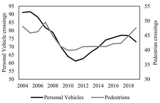
Figure 1.
Annual pedestrian and personal vehicle crossings from 2004 to 2019 (millions). Note: Annual data for the 2004–2019 period. Data in millions. Pedestrian crossings are on the right vertical axis. Source: Own estimations using data from the Bureau of Transportation Statistics.
A substantial decline is registered for personal vehicle crossings after 2005, reaching a minimum in 2010 (from 91.5 million crossings in 2005 to 39.9 million in 2010). However, this was followed by a recovery of close to 77 million crossings, which is similar to the 2008 level. Figure 1 depicts periods where pedestrian crossings improved while personal vehicles decreased, suggesting that various factors may influence each type of crossing differently.
Fullerton and Walke [4] claimed that it is not cost effective for pedestrians to shop for specific retail goods categories or travel beyond the immediate border zone. Cross-border shopping requires the price differential of the local and foreign countries to exceed the transaction costs of purchasing across the border. Therefore, as Chandra et al. [5] pointed out, border shoppers live near the border. Baruca and Zolfagharian [6] demonstrated that hedonic shopping motivation may influence economic agents (e.g., consumers) to cross the border to seek fun and pleasure experienced in cross-border shopping trips.
The primary goal of this study was to investigate the impact that people’s sentiments toward crossing the border have on personal vehicle and pedestrian crossings throughout the entire US–Mexico border. This study stems from behavioral economics studies that have examined the relationship between economic agents’ sentiments and economic variables. In those studies, various proxies for assessing investor sentiment were developed, and they can be categorized based on the source of data employed [7]. In this analysis, the use of proxies with data extracted from the volume of internet searches is proposed. The hypothesis to be tested is that policies towards illegal immigration influence the sentiment of economic agents at the aggregate level and thus affect the northbound border crossing of pedestrians and personal vehicles along the US–Mexico border.
This study also builds on prior research examining the determinants of border crossings between Mexico and the U.S. This study makes three significant contributions to the literature. First, data on border crossings were retrieved from all the U.S. Ports of Entry (PoEs) along the US–Mexico border and grouped into three regions. Second, it used sentiment variables built from the volume of internet search queries as a proxy to assess decision-makers’ sentiments. Lastly, a rolling regression analysis was performed to examine the relationship between the sentiment variables and border crossings over time.
The rest of this paper proceeds as follows. The literature review is examined in the next section. Then, in the third section, the variables and data are described. Section 4 presents the method used in the study, and the results are presented in Section 5. The discussion and trends for future research are proposed in Section 6, and the conclusion is presented in the last section.
2. Literature Review
The US–Mexico border region is home to approximately 14 million people concentrated in 14 border-city pairs. Quintana et al. [8] documented that these binational urban areas range from larger metropolitan areas, such as San Diego-Tijuana (2.9 million people), to minor city pairs, such as Nogales in Arizona and Nogales in Sonora (0.2 million). The border is shared by four U.S. states and six Mexican states. The border is 3200 km long and includes 39 Mexican municipalities, 25 U.S. counties, and 25 land ports. In 2019, close to 47.5 million pedestrians crossed northbound, and 73 million personal vehicle crossings were registered.
2.1. Border-Crossing Literature: General Overview
Heyman [9] defined a port of entry (PoE) as nodes in the world trade system where people and goods enter a nation. According to Quintana et al. [8], personal vehicle and pedestrian crossings have increased substantially since NAFTA was signed. Population growth, Mexican border industrialization, and commerce expansion are important factors in explaining the increase in crossings during this period. In addition, Lee and Wilson [10] pointed out that more than 70% of the bilateral trade between the U.S. and Mexico flows through the border’s land ports. Tourism is another important driver. According to Lee and Wilson [10], approximately 85% of Mexican tourists arrive in the U.S. through land ports, impacting the economy of border cities in the U.S.
The border-crossing literature has analyzed the relationship between border crossings and the real exchange rate [5,11,12,13,14], GDP [13,15], gasoline prices [16], unemployment [4,17], personal income [18,19], trade agreements [17,20], and geopolitical and security issues, such as the 9/11 event [20,21,22,23], and the economic impact of foreign visitors in border cities [24,25].
2.2. The US–Mexico Border
Patrick and Renforth [26] found that the devaluation of the Mexican peso affects Texas retailers, showing their reliance on Mexican customers (economic agents). Moreover, the influence of currency rate fluctuations differs by city, distance from the border, retail sector, and domestic market size. Mexican consumption is determined by purchasing power after considering currency conversion, inflation, interest rates, and available disposable income.
Gerber [27] investigated the influence of Mexican tourists on retail sales in eight U.S. border counties by employing the simple compound growth model of retail sales. According to the research, currency fluctuations impact retail sales, with nondurable goods, fashion merchants, and general merchandize outlets being more vulnerable. Fullerton [14] examined the relationship between the exchange rate and the cross-border flows in three international bridges in El Paso. He used monthly data for same-day personal vehicle, passenger, and pedestrian trips; the exchange rate; and the consumer price index. The data revealed each bridge’s border-crossing behavior. The findings demonstrate that crossing flows are not random, and peso devaluation has a varying effect on traffic on each bridge. The Mexican peso’s depreciation negatively impacts the bridge in that more personal vehicles cross, although it has a positive effect on the bridge where pedestrians prevail.
Fullerton et al. [28] studied how toll tariffs and currency exchange rates influence border crossings using 1990–2006 monthly pedestrian, personal vehicle, and cargo crossing data. The authors found a negative relationship between the toll and flow of border crossings using ARIMA transfer functions. They also found a negative relationship in land ports where pedestrians and personal vehicles predominate and a positive relationship in ports where cargo crossings dominate.
Cabral et al. [13] analyzed the relationship between exchange rate and personal vehicle passenger crossings in the 9 most active PoEs using monthly data from 1997 to 2018. Using panel data fixed effects and augmented mean group models and controlling for the difference in economic growth rates between Mexico and the U.S., they found a negative relationship between the exchange rate and border crossings and an increase in crossings when the Mexican economy improves faster than the U.S. economy.
2.3. The U.S.–Canada Border
Di Matteo and Di Matteo [19] used quarterly data about same-day vehicle crossings to examine the determinants of cross-border shopping for 7 Canadian provinces that share a border with the U.S. from 1979 to 1992. The authors employed the Gerber [27] demand model and estimated a log–log model using ordinary least squares regression techniques. They found that the main factor for border crossings in several Canadian provinces is the exchange rate. Moreover, the per capita income variable is the most important determinant; however, British Columbia’s gas price is the most relevant variable that explains border crossings.
2.4. Decision-Maker Sentiment
Traditional economic theories leave no room for irrational behavior; they assume that decisions are made through rational decision-making processes [29], and economic agents consider all publicly available information when making decisions [30]. However, empirical evidence reveals that agents are constrained in the amount of information they can process [31], questioning the rationality assumptions in classical theory. Furthermore, behavioral economics has highlighted the relevance of economic agents’ sentiments in financial markets [7], and their behavioral biases, which lead to overly optimistic/pessimistic beliefs and drive an irrational behavior [32].
The literature provides several definitions for the term “sentiment”. In the financial literature, investor sentiment is commonly characterized as either the proclivity to take risks and speculate or the overall sense of optimism or pessimism toward risky assets [33]. For example, De Long et al. [34] related sentiment to noise trading. In contrast, Baker and Wurgler [35] attribute it to feelings of optimism or pessimism about risky assets.
Scholars have devised various proxies for measuring the sentiments of economic agents, especially investors. Based on the data source from which the proxy is extracted, Zhang et al. [7] grouped these proxies into three categories. Indirect proxies are based on stock market data and survey results. Baker and Wurgler [35] used six proxies for sentiment retrieved from the stock market, including the closed-end fund discount and NYSE share turnover. Based on noise-trader sentiment models, Lemmon and Portniaguina [36] employed the University of Michigan survey of consumer sentiment and the Conference Board survey of consumer confidence as proxies for investor sentiment.
Da et al. [37] suggested that earlier indirect sentiment measures do not capture all decision-makers’ sentiments. They claimed that market-based indicators can capture more than investors’ sentiments. Moreover, survey-based proxies are infrequent, and respondents cannot be incentivized to submit truthful answers. Because of this, they stated that the volume of internet search inquiries should be used to create direct sentiment indicators.
Emerging literature has applied internet search volume data as a source to construct proxies of economic and noneconomic variables [38]. For example, Ettredge et al. [39] analyzed the relationship between the search volume of employment-related terms with monthly U.S. unemployment data. Ginsberg et al. [40] used Google search volume to predict the incidence of influenza diseases. Choi and Varian [41] used search volume from Google to estimate macroeconomic variables, including automobile sales, initial claims for unemployment benefits, travel destination planning, and consumer confidence. Guzman [42] employed search query data to examine inflation expectations. Vosen and Schmidt [43] constructed a private consumption measure based on search queries. Finally, Da et al. [37] hold that sentiment at the market level can be measured using search volume data. Thus, using online searches relevant to households in the U.S., the authors developed a Financial and Economic Attitudes Revealed by Search (FEARS) index.
In this study, it is important to emphasize that the primary goal was to explore the relationship between people’s sentiment to cross the border at the aggregate level and its effect on border crossings. This study proposes that online search query volume data should be used to develop a direct measure, based on the claim of Ettredge et al. [39] that people’s search behavior reveals information about their needs, desires, preferences, and concerns. As Guzman [42] proposed, search behavior can be interpreted as a measure of disclosed expectations. According to Da et al. [37], aggregating search volume data reveals market-level sentiment connected to specific topics. Moreover, Google search volume data is used as to gauge people’s intentions and concerns over crossing the border.
3. Data Analysis
The Bureau of Transportation Statistics provides monthly statistics for inbound crossings between the U.S. and Mexico at the PoE level. The data are classified by port, state, and means of transportation. In this study, the dependent variables were the monthly number of pedestrians and the personal vehicle crossings from Mexico to the U.S.
All PoEs were grouped into three regions: California, Texas, and other (Arizona and New Mexico). Table 1 presents the descriptive statistics of pedestrians and personal vehicles aggregated by region. In 2019, California accounted for 42.6% of the pedestrian crossings (42.9% for personal vehicle); Texas, 41.8% (44.1%); and Arizona and New Mexico, 15.6% (13%).

Table 1.
Descriptive statistics of pedestrians and personal vehicles crossing the border from Mexico to the U.S. (2004-2M2020).
Google is the largest and most popular search engine on the internet, and since 2004, it has provided the Google Trends services, in which the historical Search Volume Index (SVI) of search terms can be downloaded [37]. This tool provides the search volume of each term in hourly, daily, weekly, or monthly frequencies. In addition, the SVI data for each keyword within a particular geographical region is scaled from 0 to 100 by the period’s maximum.
To test the effect that an “anti-immigrant environment” has on economic agents’ sentiments (e.g., shopping-trip travelers) and, hence, on their attitudes and decisions toward northward pedestrian and personal vehicle crossings along the US–Mexico border, it is proposed that two variables should be constructed as proxies to capture the phenomenon from both sides of the border. According to Ettredge et al. [39] and Guzman [42], people’s search behavior can be expected to reveal matters relevant to them. These variables are derived from the Google Trends database.
If hedonic shopping drives economic agents to cross the border to pursue fun and enjoyment [6], it is reasonable to expect that an “anti-immigrant environment” in the U.S. border cities will affect economic agents’ attitudes and sentiments toward crossing the border for shopping trips, thereby influencing border crossings. Therefore, it is proposed that a variable that captures the sentiments of these economic agents at the aggregate level should be developed using the online search volume data as a proxy for their concerns about and interests in the Mexican side of the border. Based on the online activity of economic agents in the U.S., a second variable was introduced to reflect the “anti-immigrant environment” in the U.S.
For the first variable, different monthly SVI data of border-crossing-related terms, including terms associated with border crossings and migration (e.g., “tiempo de cruce,” “puente internacional,” and “cruce fronterizo”), were individually retrieved using the Google Trends tool; the search was restricted to Mexico and the period analyzed. It was followed by a “snowball technique”, which was implemented by including the related terms that Google Trends suggests in the analysis. After analyzing the stationarity and correlation of the time series of the SVI of each term with the border-crossings data, the more significant search terms were identified, which are “migrantes”, “deportaciones”, “muro fronterizo”, “border patrol”, and “patrulla fronteriza”. Lastly, the SVI of these terms is grouped by adding each month’s values to construct a single index named Border Economic Migrant Sentiment (BEMS). Because the BEMS variable comprises search terms related to security and “anti-immigration” issues, it is expected that it will capture people’s concerns about crossing the border [39,42].
The SVI of terms related to border crossings is also explored, with the geographic scope limited to the U.S. A similar research strategy is employed for the other variables, with the “immigration” search term being the most relevant. It is assumed that when an anti-immigration sentiment occurs in the U.S., the SVI of the “immigration” search term will increase. Therefore, adding the “immigration” variable (Imm) may help determine whether a rise in the hostile environment in the U.S. toward immigration may influence northbound border crossings.
Table 2 displays statistics for the main variables. The monthly average crossings for pedestrian and personal vehicles are 3.6 and 6.2 million, respectively. Figure 2 depicts the northbound border crossings for pedestrians and personal vehicles grouped by region. The annual pedestrian crossings are depicted in Figure 2a. The other region experienced a rising trend from 2004 to 2007, followed by a significant decline, which was most likely caused by the global financial crisis, reaching a minimum in 2014. Subsequently, the border crossings experienced a sluggish recovery, with nearly 7 million crossings flattening in recent years. An annual decrease in pedestrian crossing is recorded from 2004 to 2009 in the Californian PoEs, with a temporary recovery in 2007. Texan ports reported similar behavior, with border crossings declining from 2004 to 2011 and with a temporary increase in 2007.
Table 2.
Descriptive statistics of the main variables (2004-2M2020).
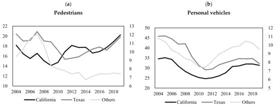
Figure 2.
Northbound PoE’s annual pedestrian and personal vehicle crossings by regions, from 2004 to 2019 (million). Note: The annual data are from 2004 to 2019 and are in millions. In Figures (a) and (b), the crossings for other are on the right vertical axis. Source: Own estimations using data from the Bureau of Transportation Statistics.
From 2009 to 2011, although pedestrian crossings in Californian ports increased, those in Texas decreased. However, from 2012 to 2015, there was a decrease in pedestrian crossings in California ports. The reverse is observed in Texas, where crossings in 2019 were lower than those registered 15 years earlier. This could indicate that regional factors may influence pedestrian border crossings.
Figure 2b exhibits the personal vehicle border crossings for each region. From 2004 to 2011, all 3 regions experienced a similar declining trend. However, a recovery was registered from 2011 to 2017 in all regions, followed by a downward pattern in the last years of the sample.
Following the literature [13,14,26,27,28], the real exchange rate movements are expected to explain the evolution of border crossings. For example, a depreciation of the Mexican peso makes shopping and leisure activities more costly, reducing the number of pedestrian and personnel vehicles crossings. Likewise, two variables are introduced to capture economic factors. First, the Global Indicator of Economic Activity (IGAE) variable is used to track the Mexican economic cycle. Second, the real U.S. gas price is used to measure its influence in border-crossing fluctuations. The gas price difference between the U.S. and Mexico is a relevant variable for passenger vehicles crossings, especially across the Texas border. Moreover, the difference tends to be positive, influencing the crossing of Mexican citizens to the U.S. to look for cheaper gas, when such price differences are significant.
The data on the exchange rate between the Mexican peso and the U.S. dollar are retrieved from Banco de Mexico (Mexican Central Bank), which publishes a monthly real exchange rate index based on a weighted basket of numerous currencies. The gas price is retrieved from the U.S. Energy Information Administration. In this study, the monthly retail gasoline prices of all grades of formulations in the U.S. are used. The data are adjusted in real terms.
The monthly IGAE indicator and the real exchange rate from 2004 to February 2020 are displayed in Figure 3. The Mexican economy experienced an upper trend during this period, which was caused by trade liberalization and other economic reforms. However, the figure reveals that during the 2008 global financial crisis, the Mexican economy suffered a slowdown pattern, with the Mexican peso depreciating significantly. As a result, from 2016 onwards, the economy and the real exchange rate experienced a sideways trend, reducing the economic growth rate as compared with that of the previous years.
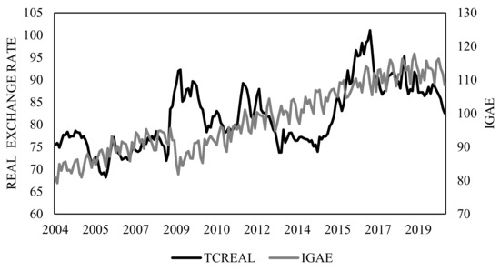
Figure 3.
IGAE and Real Exchange Rate from 2004 to 2020. Note: The monthly data are from 2004 to February 2020. IGAE stands for the Global Indicator of Economic Activity and is displayed on the right vertical axis. Source: Own estimations using data from INEGI and Banco de Mexico.
A dummy variable is included in the econometric model to capture the exogenous events that impacted the U.S. and may influence border crossings. The information about the U.S. economic recessions is retrieved from the National Bureau of Economic Research (NBER). Regarding the D_US_CRISIS variable, from December 2007 to June 2009 (including the 2008 global financial crisis) is assigned a value of 1.
Table 3 presents the correlation matrix of the dependent and the main independent variables. The real exchange rate’s negative sign regarding pedestrians and personal vehicles is as expected. Hence, there is some initial evidence that northbound border crossings decline when the Mexican peso depreciates. In the case of pedestrians and personal vehicles, the IGAE coefficient is negative, although the correlations are small. Furthermore, as projected, the real gas price is negative for personal vehicles. Lastly, the correlation between the two Google Trend variables is 0.408.
Table 3.
Correlation matrix.
4. The Empirical Model
The empirical model proposed in this study, which uses a log–log specification, closely follows the study of Di Matteo and Di Matteo [19]:
where the dependent variable denotes the t month total number of pedestrian or personal vehicle crossings. In Equation (1), Exch rate represents the real exchange rate variable, GR denotes the Mexican economy growth rate, GAS is the real gas price in the U.S., D_US_CRISIS is the dummy variable that captures economic turmoil, and represents the variables constructed from Google Trends that capture decision-maker’ sentiments (BEMS and Imm variables). The time series was computed in logarithms for both the dependent and independent variables, except the dummy variable.
Two sets of models were estimated: the first was for the entire sample of PoEs, and the second set was divided into three regions (California, Texas, and other). Endogeneity is not expected to be a concern because exchange rates are defined in international financial markets. Therefore, border crossings from Mexico are not expected to directly affect the value of the Mexican peso. Furthermore, these border crossings can have little effect on national gas prices in the U.S. or the evolution of Mexico’s national economy.
The log–log specification allowed us to identify the elasticities between the pedestrian and personal vehicle crossings and the independent variables. Due to the wealth effect resulting from the currency movements, it was expected that a depreciation of the local currency would negatively affect Mexicans’ propensity to cross northbound. Thus, it was anticipated that the sign of the coefficient estimated would be .
When the Mexican economy expands, its residents have more resources to cross northbound to take advantage of price differences in goods and services on both sides of the border [26]. Indeed, border crossings are explained by Mexican residents’ shopping trips [26,44]. Mexicans have greater resources for cross-border shopping trips near the top of the economic cycle. Thus, the coefficient of this variable was predicted to be .
For decades, the government set gas prices in Mexico, with price differentials expected along the border [4,16,19]. Thus, it can be assumed that the U.S. gas price may play a role in the decision to cross the northbound border. If the U.S. gas price increases, Mexicans are less motivated to cross the border. The sign for this coefficient was expected to be .
Based on previous studies that used people’s online search activity as a proxy for their sentiment [33,37,45,46], it can be argued that people’s sentiment may influence border-crossing fluctuations. An increase in the negative sentiment about Mexicans and immigration in the U.S. will result in fewer border crossings. If the variables based on Google Trends data captured the negative sentiments about border crossings, a negative relationship was anticipated (.
5. Results
We begin by revisiting the series’ stationarity before estimating the empirical model presented in Section 4 of this study. The primary estimations are then reported by border-crossing type and region, followed by robustness checks.
5.1. Testing for Stationarity
Table 4 reports the stationarity tests of the main dependent and independent variables in logarithms for both levels and the first differences. The Augmented Dicky Fuller (ADF) unit root tests were conducted, and the results are recorded in the first column of Table 4. The ADF tests the null hypothesis that a time series has a unit root against the alternative hypothesis that it is I (0). The level variables are presented in the first panel, revealing that the data are not stationary. The Phillips–Perron (P.P.) unit root test was also performed, and the results are reported in the second column of Table 4. For this unit root test, the null and alternative hypotheses were the same as those of the ADF test. The results indicate that the data in levels are not stationary. Therefore, the data were computed in its first difference to minimize the nonstationary problems. The data in the first differences are stationary and reported in the second column of Table 4. Stationarity tests for the individual time-series components of the border-crossing sentiment index were performed, which are stationary at the first difference (the results are not presented in Table 4 but are available on request).
Table 4.
Unit root tests.
5.2. Main Estimates
The results of the regressions of Equation (1) for personal vehicle and pedestrian crossings are presented in Table 5. The Newey–West method was used to compute the robust standard errors to account for autocorrelation problems. The results support the negative relationship between border crossings and real exchange rates. The coefficients range from −0.19 to −0.48 (at least with a significance level of 10%) for pedestrian and personal vehicle crossings. Therefore, the depreciation of the Mexican currency negatively influences the propensity to cross northbound. An increase of 1% in the exchange rate leads to approximately a −0.20% decrease in personal vehicle crossings, and that of pedestrians is close to −0.40%.
Table 5.
Personal vehicles and pedestrians OLS estimations (period: 2004–2020M02).
The coefficient of the IGAE variable is positive (1% significance level), as expected. Thus, Mexicans tend to cross northbound more frequently when they have more resources. With an increase of 1% in the IGAE indicator, increases closes to 1% in personal vehicle crossings and 1.4% in pedestrian crossings are expected. Thus, the elasticities for IGAE are somewhat higher for pedestrian crossings than personal vehicles. These differences are statistically significant (1% significance level). To conduct this analysis, the Stata’s suest-based test of equality of coefficients was utilized, by comparing the d(lnIGAE) coefficients of model 1 to model 4, model 2 to model 5, and model 3 to model 6 (Table 5). Moreover, there is no evidence that the price of gasoline in the U.S. is a motive for Mexican residents to cross the border.
In Table 5, the BEMS index variable is added to models 1 and 4, the immigration variable is added to models 2 and 5, and both variables are included in models 3 and 6. The coefficient of both variables is negative, as predicted. An increase of 1% in the BEMS index leads to a 0.02% decrease in border crossings. Moreover, a 1% increase in the Imm leads to an approximately 0.07% decrease in northbound border crossings. By comparing the d(ln Imm) coefficients calculated using models 2 and 5 in Table 5, which is significant at the 10% level, it is found that Imm is slightly larger for pedestrian crossings than for personal vehicles. These differences are statistically significant (5% significance level), using the Stata’s suest-based test of equality of coefficients. After examining models 3 and 6, we find that the coefficients of Imm are larger than the coefficients of the BEMS index for both pedestrian and personal vehicle crossings. These differences are statistically significant (5% significance level), using the Stata’s suest-based test of equality of coefficients.
Table 6 (personal vehicle crossings) and Table 7 (pedestrian crossings) report the results for the 3 regions in which the PoEs are grouped. The BEMS index variable is included in models 1, 4, and 7 in Table 6 and Table 7; the Imm variable in models 2, 5, and 8; and both variables in models 3, 6, and 9. By analyzing both tables, some interesting insights are obtained. First, in Texas, when the Imm is added, the relationship between personal vehicle crossings and the real exchange rate is not statistically significant, and for pedestrian models, the significance reduces. Moreover, for personal vehicle models in the other two regions, the significance reduces. However, the statistical significance level of the real exchange rate does not change when Imm is included in California and other region’s pedestrian crossings models.
Table 6.
OLS regressions results of personal vehicle crossings clustered by regions (2004–2020M02).
Table 7.
Pedestrian crossings OLS regression results clustered by regions (period: 2004-2020M02).
If Imm captures some of the possible hostile immigration-related environment, an anti-immigrant environment weakens the economic motivation for crossing, especially in Texas PoEs. However, additional research may be conducted to examine this argument, as previous findings suggest a possible relationship between the real exchange rate, the anti-immigrant environment, and border crossings flow. However, such a relationship should be viewed with caution, as we provide no strong evidence to support such findings.
If tourism and shopping are two of the main reasons for Mexicans to cross the border [4,26], an increase in an anti-immigrant environment may diminish the economy of border cities.
However, in terms of elasticities, a 1% increase in Imm in Texas results in a −0.127% decline in pedestrian crossings, which is slightly greater than the −0.090% elasticity of personal vehicles. These differences are statistically significant (5% significance level), using the Stata’s suest-based test of equality of coefficients. This indicates that pedestrian crossings are more sensitive to changes in Imm.
Second, in all regions, the Mexican economic cycle represented by IGAE is statistically significant at the 1% level. As expected, when Mexicans have more resources, they cross the border more frequently. However, gas price is not statistically significant, suggesting that most people who cross the border may be motivated by shopping, tourism, or leisure activities rather than purchasing gasoline.
Lastly, except for the pedestrian models in California (Table 7), the BEMS index is statistically significant in all models. This might imply that economic motivators may be more important in influencing pedestrians’ border-crossing decisions in California than in the other regions. However, future research may further analyze this line of reasoning. By comparing models 4 in Table 6 and Table 7, it is found in Texas that the BEMS index elasticities are slightly higher for pedestrian crossings (−0.03%) than personal vehicles (−0.02%). When both sentiment variables are added, the Imm coefficient has a higher value than the BEMS index coefficient in California and Texas for both types of crossings. Models 3 and 6 in Table 6 and Table 7 were examined. These differences are statistically significant (10% significance level in California, 5% significance level in Texas), using the Stata’s suest-based test of equality of coefficients.
These results might suggest that people’s sentiments play a role in their decision to cross the border. Imm is significant in all models and regions, especially in California and Texas. If this proxy captures some of the variations in the anti-immigrant sentiment, the findings might imply that the hostile anti-immigration atmosphere may have a negative impact on border crossings and the economies of U.S. border cities.
5.3. Robustness Checks
Rolling regression analysis was conducted as a robustness check. This statistical method seeks to analyze the relationship between the dependent and independent variables. However, unlike other methods, a specific window size is defined and moved progressively along the sample period. Therefore, a window size of 24 observations was selected in this study generating 174 subsamples, which were used to perform the rolling regression with a step of 1 (Windows of 12 and 48 lengths were tested, yielding similar results that can be provided upon request). Henceforth, the window was two years long and moved progressively from one month to the next. The results can be delivered upon request. This analysis intended to evaluate the behavior of the coefficients of the BEMS and Imm variables using the following specifications:
where the dependent variables and denote the t month total number of personal vehicle and pedestrian crossings. In Equations (2) and (3), Exch rate represents the real exchange rate and GR denotes the Mexican economy growth rate; in Equation (2) GAS is the U.S. real gas price, and denotes the BEMS and Imm variables.
Figure 4a depicts the coefficients for the first difference of the BEMS logarithm for personal vehicle crossings. Throughout the period, the BEMS had a negative relationship with personal vehicles. However, short-run episodes with positive coefficients arose, such as the summer of 2012 and the 2013 and 2014 winter seasons. Pedestrian crossings followed a similar pattern (Figure 4c). Although Figure 4a depicts 2 main downward trends—one from 2006 to 2008 and the other from 2014 to 2019—with the latter coinciding with the Donald Trump Administration, a similar pattern was found for pedestrian crossings. The mean of the d(ln BEMS) coefficients for personal vehicle (pedestrian) crossings was −0.031 (−0.041), with a standard deviation of 0.020 (0.027), suggesting that pedestrian crossings are slightly more sensitive to fluctuations in the BEMS index than personal vehicles.
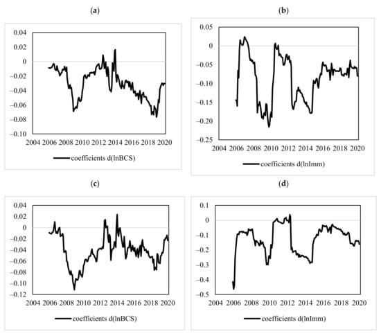
Figure 4.
Rolling regression coefficients for the BEMS and Imm variables (24-month window). (a) Dependent variable: LN personal vehicles; (b) Dependent variable: LN personal vehicles; (c) Dependent variable: LN pedestrians; (d) Dependent variable: LN pedestrians.
Figure 4b reveals that the coefficients of the first difference of the Imm logarithm for personal vehicle crossings are negative, except from January 2006 to May 2007 and 2 subperiods in 2010. Two rising trends were followed by major decreases in 2006 and 2010. In addition, a low point is observed in 2014, coinciding with the 2014 immigration crisis. Due to violence and persecution, an increasing number of Central American families seek asylum in the U.S. [47]. Similar behavior is observed in Figure 4d for pedestrian crossings. The coefficients are more stable in recent years, as seen in Figure 4b for personal vehicle crossings, whereas pedestrian crossings (Figure 4d) experienced a downward trend. In the case of personal vehicle (pedestrian) crossings, the mean of the coefficients of d(ln Imm) was −0.085 (−0.125), with a standard deviation of 0.059 (0.094). These findings might imply that pedestrian crossings are more responsive to Imm.
The 4 panels in Figure 4 depict a rise in the elasticity between the BCI and Imm and border crossings during the 2008 and 2012 economic slumps, as demonstrated by the downtrend of the IGAE indicator in Figure 3. This suggests that sentiments may have a larger influence on the choice to cross the border during economic turmoil.
6. Discussion
The topics examined in this study may be relevant to those overseeing the economic development of the US–Mexico border regions. This manuscript reveals that the U.S. authorities can have an impact on Mexicans’ intention to cross the border based on their perception of the new developments of U.S. immigration policies. It is observed that controlling for economic factors, such as the real exchange rate and economic activity, border crossings are also affected by the sentiments of people toward new immigration policies. Even when those policies have, in principle, no impact on legal immigration, how people perceive policy changes affects their willingness to cross the northbound border. The findings are relevant for communities in the U.S. that receive a significant number of visitors from Mexico.
This study also offers some potential lines of further research. COVID-19 has changed the dynamics of border crossings. Nowadays, Mexican pedestrians and personal vehicles have new reasons to visit the U.S. border regions. This is because the U.S. government is ahead of the Mexican government in the COVID-19 vaccination. Moreover, the situation has not precluded Mexican citizens from obtaining a vaccine in the U.S. before taking it in their own country. The U.S.–Mexican border was closed in March 2020 but opened in November 2021. This offers new motives for Mexicans for crossing, which are to look for booster shots, to be immunized with the vaccine of their choice, or to obtain vaccines for the underage population, whom the Mexican government has been reluctant to include in its vaccination policies. These new motives can also complement the previous motives for crossings discussed in this study. Indeed, the impact of closing and opening the border can also offer an interesting setting for testing hypotheses about the nature of border crossings along the US–Mexico border.
7. Conclusions
This study tested the hypothesis that the anti-immigrant environment in the U.S. may influence the sentiment of economic agents and thus affect the crossings along the US–Mexico border. Unlike previous studies, variables constructed from online search volume data were used. In addition, a rolling regression analysis was performed to examine the relationship between the sentiment variables and border crossings over time. Finally, all the PoEs along the border were included and grouped into three geographic regions.
The elasticities obtained suggest a negative relationship between the real exchange rate and both types of border crossings, which is consistent with previous literature that indicates that the depreciation of the Mexican peso has an adverse effect on border crossings. The influence of the Mexican economic cycle was slightly more significant for pedestrians (1.39%) than personal vehicle crossings (1.09%). Therefore, the border is crossed more frequently when the Mexican economy grows.
When Imm was included, the relationship between the real exchange rate and personal vehicle crossings was not statistically significant in Texas; this might imply that an anti-immigrant environment reduces the economic incentive for crossing. In contrast, for the pedestrian crossings in California, the inclusion of Imm did not reduce the statistical significance.
Following the studies of Ettredge et al. [39] and Guzman [42], it can be argued that the BEMS index variable is expected to capture people’s sentiment to cross the border at the aggregate level. The BEMS was statistically significant in all models for both crossings, except pedestrians in California, which might indicate that the other factors analyzed have a greater influence in this region than the sentiment captured by the BEMS.
As suggested by Baruca and Zolfagharian [6], if a hedonic shopping motive drives customers to cross the border to pursue fun and enjoyment, the preceding findings may have some practical implications. Border crossings in Texas are more sensitive to changes in the anti-immigration environment and people’s sentiment, as captured by the BEMS index; hence, it is vital to implement public policies that enhance a friendlier environment for those interested in crossing the border because of the economic impact of Mexicans’ shopping trips on the U.S. border-city economies [25].
The rolling regression results demonstrate that the relationship between the sentiment proxy variables and border crossings is negative, except for short-run subperiods, which are positive, although with small coefficients. Thus, pedestrian crossings are more sensitive to changes in the sentiment proxy variables than personal vehicles. In addition, the elasticities of the sentiment proxy variables and border crossings increase during economic turmoil.
Author Contributions
Conceptualization and methodology, R.C., F.G.-F. and E.S.; software, F.G.-F.; validation and formal analysis, R.C., F.G.-F. and E.S.; data curation, F.G.-F.; writing—original draft preparation, F.G.-F.; writing—review and editing, R.C., F.G.-F. and E.S.; supervision, R.C. and E.S. All authors have read and agreed to the published version of the manuscript.
Funding
This research received no external funding.
Institutional Review Board Statement
Not applicable.
Informed Consent Statement
Not applicable.
Data Availability Statement
The data presented in this study are available on request from the corresponding author.
Conflicts of Interest
The authors declare that they have no known competing financial interests or personal relationships that could have appeared to influence the work reported in this paper.
References
- Labastida-Tovar, E. The impact of NAFTA on the Mexican-U.S. border region. In The Politics, Economics, and Culture of Mexican-U.S., 1st ed.; Ashbee, E., Clausen, H.B., Pedersen, C., Eds.; Palgrave Macmillan: New York, NY, USA, 2007; pp. 107–132. [Google Scholar]
- Nicita, A. Who benefited from trade liberalization in Mexico? Measuring the effects on household welfare. In Policy Research Working Paper, No.3265; The World Bank: Washington, DC, USA, 2004. [Google Scholar]
- Hanson, G. What Has Happened to Wages in Mexico since NAFTA? National Bureau of Economic Research: Cambridge, MA, USA, 2003. [Google Scholar] [CrossRef]
- Fullerton, T.M.; Walke, A.G. Cross-Border Shopping and Employment Patterns in the Southwestern United States. J. Int. Commer. Econ. Policy 2019, 10, 1950015. [Google Scholar] [CrossRef]
- Chandra, A.; Head, K.; Tappata, M. The Economics of Cross-Border Travel. Rev. Econ. Stat. 2014, 96, 648–661. [Google Scholar] [CrossRef]
- Baruca, A.; Zolfagharian, M. Cross-Border Shopping: Mexican Shoppers in the US and American Shoppers in Mexico: Cross-Border Shopping. Int. J. Consum. Stud. 2013, 37, 360–366. [Google Scholar] [CrossRef]
- Zhang, W.; Li, X.; Shen, D.; Teglio, A. Daily Happiness and Stock Returns: Some International Evidence. Physica A 2016, 460, 201–209. [Google Scholar] [CrossRef]
- Quintana, P.J.E.; Ganster, P.; Stigler Granados, P.E.; Muñoz-Meléndez, G.; Quintero-Núñez, M.; Rodríguez-Ventura, J.G. Risky Borders: Traffic Pollution and Health Effects at US–Mexican Ports of Entry. J. Borderl. Stud. 2015, 30, 287–307. [Google Scholar] [CrossRef]
- Heyman, J. Ports of Entry as Nodes in the World System. Identities 2004, 11, 303–327. [Google Scholar] [CrossRef]
- Lee, E.; Wilson, C.E. The state of trade, competitiveness and economic well-being in the US-Mexico border region. In Border Research Partnership Working Paper; Wilson Center Mexican Institute: Washington, DC, USA, 2012. [Google Scholar]
- Baggs, J.; Fung, L.; Lapham, B. Exchange Rates, Cross-Border Travel, and Retailers: Theory and Empirics. J. Int. Econ. 2018, 115, 59–79. [Google Scholar] [CrossRef] [Green Version]
- Bello, P. Exchange rate fluctuations and border crossings: Evidence from the Swiss-Italian border. In IdEP Economic Papers; USI Università Della Svizzera Italiana: Lugano, Switzerland, 2017. [Google Scholar]
- Cabral, R.; Mollick, A.V.; Saucedo, E. Northbound Border Crossings from Mexico to the U.S. and the Peso/Dollar Exchange Rate. Res. Transp. Bus. Manag. 2019, 33, 100423. [Google Scholar] [CrossRef]
- Fullerton, T.M., Jr. Currency Movements and International Border Crossings. Int. J. Public Adm. 2000, 23, 1113–1123. [Google Scholar] [CrossRef]
- Anderson, W.P.; Maoh, H.F.; Burke, C.M. Passenger Car Flows across the Canada–US Border: The Effect of 9/11. Transp. Policy (Oxf.) 2014, 35, 50–56. [Google Scholar] [CrossRef]
- Fullerton, T.M., Jr.; Jiménez, A.A.; Walke, A.G. An Econometric Analysis of Retail Gasoline Prices in a Border Metropolitan Economy. N. Am. J. Econ. Financ. 2015, 34, 450–461. [Google Scholar] [CrossRef]
- Adkisson, R.V.; Zimmerman, L. Retail Trade on the U.S.-Mexico Border during the NAFTA Implementation Era. Growth Chang. 2004, 35, 77–89. [Google Scholar] [CrossRef]
- Burke, C.M. A Comparative Analysis of Cross Border Travel Influences at the Port Level: Pacific Highway/Douglas, B.C.—Blaine, WA and Windsor, ON—Detroit, MI. Res. Transp. Bus. Manag. 2015, 16, 95–101. [Google Scholar] [CrossRef]
- Di Matteo, L.; Di Matteo, R. An Analysis of Canadian Cross-Border Travel. Ann. Tour. Res. 1996, 23, 103–122. [Google Scholar] [CrossRef]
- Andreas, P. A Tale of Two Borders: The U.S.-Mexico and U.S.-Canada Lines after 9/11; Center for Comparative Immigration Studies, University of California at San Diego: La Jolla, CA, USA, 2003. [Google Scholar]
- Bradbury, S.L. The Impact of Security on Travelers across the Canada–US Border. J. Transp. Geogr. 2013, 26, 139–146. [Google Scholar] [CrossRef]
- Ferris, J.S. Quantifying Non-Tariff Trade Barriers: What Difference Did 9/11 Make to Canadian Cross-Border Shopping? Can. Public Policy 2010, 36, 487–501. [Google Scholar] [CrossRef]
- Fullerton, T.M., Jr.; Walke, A.G. Homicides, Exchange Rates, and Northern Border Retail Activity in Mexico. Ann. Reg. Sci. 2014, 53, 631–647. [Google Scholar] [CrossRef]
- Charney, A.H.; Pavlakovich-Kochi, V.K. The Economic Impacts of Mexican Visitors to Arizona. In Economic and Business Research Program; Eller College of Business and Public Administration, University of Arizona: Tucson, AZ, USA, 2002. [Google Scholar]
- Ghaddar, S.; Brown, C.J. The Economic Impact of Mexican Visitors along the US-Mexico Border: A Research Synthesis; University of Texas-Pan American: Edinburg, TX, USA, 2006; pp. 1–20. [Google Scholar]
- Patrick, J.M.; Renforth, W. The Effects of the Peso Devaluation on Cross-border Retailing. J. Borderl. Stud. 1996, 11, 25–41. [Google Scholar] [CrossRef]
- Gerber, J. The Effects of a Depreciation of the Peso on Cross-Border Retail Sales in San Diego and Imperial Counties; University of California San Diego: San Diego, CA, USA, 1999. [Google Scholar]
- Fullerton, T.M., Jr.; Molina, A.L., Jr.; Walke, A.G. Tolls, Exchange Rates, and Northbound International Bridge Traffic from Mexico. Reg. Sci. Policy Pract. 2013, 5, 305–321. [Google Scholar] [CrossRef] [Green Version]
- Sharpe, W.F. Capital Asset Prices: A Theory of Market Equilibrium under Conditions of Risk. J. Financ. 1964, 19, 425–442. [Google Scholar] [CrossRef] [Green Version]
- Fama, E.F. The Behavior of Stock-Market Prices. J. Bus. 1965, 38, 34–105. [Google Scholar] [CrossRef]
- Simon, H.A. Bounded Rationality. In Utility and Probability; Palgrave Macmillan UK: London, UK, 1990; pp. 15–18. [Google Scholar] [CrossRef]
- Ofek, E.; Richardson, M. DotCom Mania: The Rise and Fall of Internet Stock Prices. J. Financ. 2003, 58, 1113–1137. [Google Scholar] [CrossRef] [Green Version]
- Qadan, M.; Nama, H. Investor Sentiment and the Price of Oil. Energy Econ. 2018, 69, 42–58. [Google Scholar] [CrossRef]
- De Long, J.B.; Shleifer, A.; Summers, L.H.; Waldmann, R.J. Noise Trader Risk in Financial Markets. J. Polit. Econ. 1990, 98, 703–738. [Google Scholar] [CrossRef]
- Baker, M.; Wurgler, J. Investor Sentiment and the Cross-Section of Stock Returns. J. Financ. 2006, 61, 1645–1680. [Google Scholar] [CrossRef] [Green Version]
- Lemmon, M.; Portniaguina, E. Consumer Confidence and Asset Prices: Some Empirical Evidence. Rev. Financ. Stud. 2006, 19, 1499–1529. [Google Scholar] [CrossRef]
- Da, Z.; Engelberg, J.; Gao, P. The Sum of All FEARS Investor Sentiment and Asset Prices. Rev. Financ. Stud. 2015, 28, 1–32. [Google Scholar] [CrossRef] [Green Version]
- Irresberger, F.; Mühlnickel, J.; Weiß, G.N.F. Explaining Bank Stock Performance with Crisis Sentiment. J. Bank. Financ. 2015, 59, 311–329. [Google Scholar] [CrossRef]
- Ettredge, M.; Gerdes, J.; Karuga, G. Using Web-Based Search Data to Predict Macroeconomic Statistics. Commun. ACM 2005, 48, 87–92. [Google Scholar] [CrossRef]
- Ginsberg, J.; Mohebbi, M.H.; Patel, R.S.; Brammer, L.; Smolinski, M.S.; Brilliant, L. Detecting Influenza Epidemics Using Search Engine Query Data. Nature 2009, 457, 1012–1014. [Google Scholar] [CrossRef]
- Choi, H.; Varian, H. Predicting the Present with Google Trends: Predicting the Present with Google Trends. Econ. Rec. 2012, 88, 2–9. [Google Scholar] [CrossRef]
- Guzmán, G. Internet Search Behavior as an Economic Forecasting Tool: The Case of Inflation Expectations. J. Econ. Soc. Meas. 2011, 36, 119–167. [Google Scholar] [CrossRef]
- Vosen, S.; Schmidt, T. Forecasting Private Consumption: Survey-Based Indicators vs. Google Trends. J. Forecast. 2011, 30, 565–578. [Google Scholar] [CrossRef] [Green Version]
- Diehl, P.N. The Effects of the Peso Devaluation on Texas Border Cities. Tex. Bus. Rev. 1983, 57, 120–125. [Google Scholar]
- Da, Z.; Engelberg, J.; Gao, P. In Search of Attention. J. Financ. 2011, 66, 1461–1499. [Google Scholar] [CrossRef]
- Preis, T.; Moat, H.S.; Stanley, H.E. Quantifying Trading Behavior in Financial Markets Using Google Trends. Sci. Rep. 2013, 3, 1684. [Google Scholar] [CrossRef] [Green Version]
- Musalo, K.; Lee, E. Seeking a Rational Approach to a Regional Refugee Crisis: Lessons from the Summer 2014 “Surge” of Central American Women and Children at the US-Mexico Border. J. Migr. Hum. Secur. 2017, 5, 137–179. [Google Scholar] [CrossRef]
Publisher’s Note: MDPI stays neutral with regard to jurisdictional claims in published maps and institutional affiliations. |
© 2022 by the authors. Licensee MDPI, Basel, Switzerland. This article is an open access article distributed under the terms and conditions of the Creative Commons Attribution (CC BY) license (https://creativecommons.org/licenses/by/4.0/).