Direct Position Determination of Non-Circular Sources for Multiple Arrays via Weighted Euler ESPRIT Data Fusion Method

Abstract

In recent years, direct position determination (DPD) with multiple arrays for non-circular (NC) signals is a hot topic to research. Conventional DPD techniques with spectral peak search methods have high computational complexity and are sensitive to the locations of the observation stations. Besides, there will be loss when the signal propagates in the air, which leads to different received signal-to-noise ratios (SNRs) for each observation station. To attack the problems mentioned above, this paper derives direct position determination of non-circular sources for multiple arrays via weighted Euler estimating signal parameters viarotational invariance techniques (ESPRIT) data fusion (NC-Euler-WESPRIT) method. Firstly, elliptic covariance information of NC signals and Euler transformation are used to extend the received signal. Secondly, ESPRIT is applied to avoid the high-dimensional spectral function search problem of each observation station. Then, we combine the information of all observation stations to construct a spectral function without complex multiplication to reduce the computational complexity. Finally, the data of each observation station is weighted to compensate for the projection error. The consequence of simulation indicates that the proposed NC-Euler-WESPRIT algorithm not only improves the estimation performance, but also greatly reduces the computational complexity compared with subspace data fusion (SDF) technology and NC-ESPRIT algorithm.

1. Introduction

As an important research area about signal processing, passive location has attracted extensive attention recently. It has applications in many fields including sonar, communication and astronomy [1,2,3,4]. With the development of radio technology, the electromagnetic environment becomes more and more complex which makes it hard for the conventional single antenna to extract accurate and useful information [5]. Besides, single antenna can only get the direction information of the targets without distance and other information. Instead, multiple arrays have the advantages of flexible beam control [6], higher spatial resolution [7] and higher signal gain [8]. Original two-step location technology needs to estimate the intermediate parameters from the original data, such as time of arrival (TOA) [9], time difference of arrival (TDOA) [10], angle of arrival (AOA) [11]. Then, the locations of targets can be estimated through the spatial geometric relationship [12]. Instead of estimating the intermediate parameters, DPD can directly obtain the estimation of target locations from the original data [13]. Therefore, DPD avoids the error caused by modeling the intermediate parameters and can acquire better positioning performance than original two-step location [14].

According to the elliptic covariance characteristics of the source, sources could be divided into two categories: circular sources and non-circular sources [15]. At present, a lot of research has been done on DPD algorithm of circular sources. A. J. Weiss proposed a DPD algorithm of multiple radio-frequency signals in 2004 [16]. Right after this, A. J. Weiss proposed a DPD algorithm via maximum likelihood (ML) method [17] in 2007. After some time, M. Oispuu provided a direct position determination algorithm: using ML and Capon method [18] to improve the estimation accuracy in 2010. Then, T. Qin provided a DPD algorithm with moving arrays in 2018 [19]. T. Zhou proposed an iterative adaptive direct localization technology to deal with coherent sources [20] in 2019. X. Zhang proposed a DPD technology with a moving coprime array [21] in 2021. However, many NC signals exist in modern wireless communication systems, like amplitude modulation (AM), quadrature phase shift keying (QPSK) and binary phase shift keying (BPSK) signals. Thus, it is necessary to promote the research of direct localization algorithm with NC sources. In recent years, some scholars have extended the idea of direction of arrival (DOA) estimation of NC signals to DPD of NC signals. J. Yin used the characteristics of NC sources to improve the location performance in [22,23,24]. Then, Y. Zhang and T. Qin used the features of Doppler Shifts and sparse array to further improve the location performance in [25,26,27].

However, current DPD algorithms of NC signals need to fuse the received data of each observation station for high-dimensional spectral function search, which undoubtedly has a great computational complexity. In addition, the difference of SNRs for each observation station is often large, and the impact of this difference on the estimation performance of the algorithm can not be ignored [28]. As the existing algorithms do not consider the effect of this difference, they are more sensitive to the locations of the observation stations, resulting in insufficient estimation accuracy. Thus, combined with the idea of Euler transformation [29] and elliptic covariance information of NC sources, this paper derives the Euler ESPRIT DPD algorithm for NC sources (NC-Euler-ESPRIT). As SNRs of received signals at each observation station are different, this paper introduces the principle of power allocation [30] and derives weighted Euler ESPRIT DPD algorithm for NC sources (NC-Euler-WESPRIT). The consequence of simulation shows that the proposed NC-Euler-WESPRIT algorithm not only improves the estimation performance, but also greatly reduces the computational complexity compared with SDF technology and NC-ESPRIT algorithm.

The main contributions are summarized as follows:

(1)

The proposed NC-Euler-WESPRIT DPD algorithm takes full advantage of elliptic covariance information of NC signals to expand the virtual array aperture. Compared with original two-step localization technique and SDF algorithm, NC-Euler-WESPRIT DPD increases the available degrees of freedom (DOF).

(2)

Euler transformation is applied to decrease the complexity by converting complex number calculation into real number operation and ESPRIT is applied to avoid the high-dimensional spectral function search problem of each observation station. Then we combine the information of all observation stations to construct a spectral function without complex multiplication to further reduce the computational complexity.

(3)

In practice, there will be loss when the signal propagates in the air and SNRs of received signals at each observation station are often different. Therefore, a specific weight is set to compensate for the projection error and get better positioning performance.

(4)

Complexity analysis, Cramer Rao lower bound (CRLB) and simulation consequence are given to check the effectiveness and superiority of the NC-Euler-WESPRIT DPD algorithm.

The following structure of the article is: A data model is introduced in Section 2. A NC-Euler-WESPRIT DPD algorithm is derived in Section 3. Performance analysis, simulation experiments and conclusions are put in Section 4 and Section 5, respectively. It should be noted that vectors and matrices are lower-case bold and upper-case bold, respectively; $\mathrm{diag}\left\{·\right\}$ represents diagonal matrix; $\left|\right|·\left|\right|$ represents the $l_2$ norm; $|·|$ indicates absolute value; ${\left(·\right)}^{*}$, ${\left(·\right)}^T$, ${\left(·\right)}^H$ denote conjugate, transposition and conjugate transpose, respectively; $\mathrm{Re}\left(·\right)$ and $\mathrm{Im}\left(·\right)$ denote real part and imaginary part, respectively; ${\mathit{I}}_N$ denotes N dimensional unit array; ⊗ denotes Kronecker product; $\partial \left(a\right)/\partial \left(b\right)$ stands for the derivative of a with respect to b; ${\left(·\right)}^{+}$ and ${\left(·\right)}^{-1}$ denote general Moore-Penrose inverse and the inverse of the matrix.

2. Model Formulation

For ease of illustration, Figure 1 shows the direct positioning scene with multiple arrays. Consider that there are Q unknown far-field incoherent narrowband sources impacting G known observation stations. Each observation station is outfitted with a uniform linear array (ULA) of M elements horizontally placed along x-axis and the interval between arrays is d. The number of snapshots is K. In this two-dimensional plane, we assume that the unknown target locations are ${\mathbf{p}}_q={\left[x_q,y_q\right]}^T$$\left(q=1,2,\cdots ,Q\right)$ and known positions of observation stations are ${\mathbf{u}}_g={\left[x_g,y_g\right]}^T$$\left(g=1,2,\cdots ,G\right)$. In practice, there will be loss when the signal propagates in the air [31,32]. In other words, when a target impinges on different observation stations, SNR of received signals at each observation station often varies greatly, so we define the path propagation loss coefficient as [33]

$${\alpha }_{g,q}=\sqrt{\frac{{\mathrm{P}}_{g,q}}{{\mathrm{P}}_q}},$$

(1)

where ${\mathrm{P}}_q$ and ${\mathrm{P}}_{g,q}$ stand for the power of the $q\mathrm{th}$ emitter signal and the power of the signal from the $q\mathrm{th}$ target received at the $g\mathrm{th}$ observation location, respectively. Supposing the emitter signal sent to the $g\mathrm{th}$ observation station at the $k\mathrm{th}$ sampling time from the $q\mathrm{th}$ target is $s_{g,q}\left(k\right)$. For simplicity, we only consider the signal whose non-circular rate is 1, i.e., Equation (2) is satisfied [15]

$$E\left[{\mathit{s}}_g\left(k\right){\mathit{s}}_g^H\left(k\right)\right]=e^{j\phi }E\left[{\mathit{s}}_g\left(k\right){\mathit{s}}_g^T\left(k\right)\right],$$

(2)

where $\phi$ denotes non-circular phase and ${\left(·\right)}^T$ denotes transposition. Then, the signal received by the $g\mathrm{th}$ observation station at the $k\mathrm{th}$ sampling time can be stated as [33]

$${\mathit{r}}_g\left(k\right)=\sum _{q=1}^Q{\alpha }_{g,q}\mathit{a}\left({\theta }_{g,q}\right)s_{g,q}\left(k\right)+{\mathit{n}}_g\left(k\right),$$

(3)

where ${\theta }_{g,q}$ represents DOA of the $q\mathrm{th}$ target received by the $g\mathrm{th}$ observation station,

$$\mathit{a}\left({\theta }_{g,q}\right)={\left[1,e^{-j\frac{2\pi d}{\lambda }cos{\theta }_{g,q}},\cdots ,e^{-j\frac{2\pi d}{\lambda }\left(M-1\right)cos{\theta }_{g,q}}\right]}^T\in {\mathbb{C}}^{M\times 1},$$

(4)

$\lambda$ denotes the wavelength and ${\mathit{n}}_g\left(k\right)$ denotes noise vector, which obeys Gaussian distribution. According to the previous far-field assumption, the observation station could be approximated to a point. Hence, we rewrite Equation (4).

$${\mathit{a}}_g\left({\mathit{p}}_q\right)={\left[1,e^{-j\frac{2\pi d}{\lambda }\frac{{\mathit{u}}_g\left(1\right)-{\mathit{p}}_q\left(1\right)}{\left|\right|{\mathit{u}}_g-{\mathit{p}}_q\left|\right|}},\cdots ,e^{-j\frac{2\pi d}{\lambda }\left(M-1\right)\frac{{\mathit{u}}_g\left(1\right)-{\mathit{p}}_q\left(1\right)}{\left|\right|{\mathit{u}}_g-{\mathit{p}}_q\left|\right|}}\right]}^T\in {\mathbb{C}}^{M\times 1},$$

(5)

Then, Equation (3) can be rewritten as

$${\mathit{r}}_g\left(k\right)={\mathit{A}}_g\left(\mathit{p}\right){\mathsf{\Lambda }}_g{\mathit{s}}_g\left(k\right)+{\mathit{n}}_g\left(k\right)\in {\mathbb{C}}^{M\times 1},$$

(6)

where ${\mathit{A}}_g\left(\mathit{p}\right)$, ${\mathsf{\Lambda }}_g$, ${\mathit{s}}_g\left(k\right)$ represent the direction matrix, propagation loss matrix and source vector of the $g\mathrm{th}$ observation station, respectively.

$${\mathit{A}}_g\left(\mathit{p}\right)=\left[{\mathit{a}}_g\left({\mathit{p}}_1\right),{\mathit{a}}_g\left({\mathit{p}}_2\right),\cdots ,{\mathit{a}}_g\left({\mathit{p}}_Q\right)\right]\in {\mathbb{C}}^{M\times Q},$$

(7)

$${\mathsf{\Lambda }}_g=\left[\begin{array}{cccc}{\alpha }_{g,1}& 0& \cdots & 0\\ 0& {\alpha }_{g,2}& \ddots & ⋮\\ ⋮& \ddots & \ddots & 0\\ 0& \cdots & 0& {\alpha }_{g,Q}\end{array}\right]\in {\mathbb{R}}^{Q\times Q},$$

(8)

$${\mathit{s}}_g\left(k\right)={\left[s_{g,1}\left(k\right),\cdots ,s_{g,Q}\left(k\right)\right]}^T\in {\mathbb{C}}^{Q\times 1},$$

(9)

$${\mathit{n}}_g\left(k\right)={\left[n_{g,1}\left(k\right),n_{g,2}\left(k\right),\cdots ,n_{g,M}\left(k\right)\right]}^T\in {\mathbb{C}}^{M\times 1}$$

(10)

3. The Proposed Algorithm

3.1. NC-ESPRIT-DPD

From [25], the non-circular signal can be written in the following form

$${\mathit{s}}_g\left(k\right)=\mathit{\Phi }{\mathit{s}}_g^{\left(R\right)}\left(k\right),$$

(11)

where $\mathit{\Phi }$ represents the NC phase matrix

$$\mathit{\Phi }=\left[\begin{array}{cccc}{e}^{-j{\phi }_1}& 0& \cdots & 0\\ 0& e^{-j{\phi }_2}& \ddots & ⋮\\ ⋮& \ddots & \ddots & 0\\ 0& \cdots & 0& e^{-j{\phi }_Q}\end{array}\right]\in {\mathbb{C}}^{Q\times Q},$$

(12)

$${\mathit{s}}_g^{\left(R\right)}\left(k\right)={\left[s_{g,1}^{\left(R\right)}\left(k\right),s_{g,2}^{\left(R\right)}\left(k\right),\cdots ,s_{g,Q}^{\left(R\right)}\left(k\right)\right]}^T\in {\mathbb{R}}^{Q\times 1},$$

(13)

where ${\phi }_q$ represents NC phase of the $q\mathrm{th}$ source and $s_{g,q}^{\left(R\right)}\left(k\right)$ stands for the amplitude of the signal. Thus, Equation (6) can be rewritten according to Equation (11):

$${\mathit{r}}_g\left(k\right)={\mathit{A}}_g\left(\mathit{p}\right){\mathsf{\Lambda }}_g\mathit{\Phi }{\mathit{s}}_g^{\left(R\right)}\left(k\right)+{\mathit{n}}_g\left(k\right)\in {\mathbb{C}}^{M\times 1}$$

(14)

The received signal can be extended by making full use of the elliptic covariance information of NC sources [34]:

$${\mathit{z}}_g\left(k\right)=\left[\begin{array}{c}{\mathit{r}}_g\left(k\right)\\ {\mathit{Jr}}_g^{*}\left(k\right)\end{array}\right]=\left[\begin{array}{c}{\mathit{A}}_g\mathit{\Phi }\\ {\mathit{JA}}_g^{*}{\mathit{\Phi }}^{*}\end{array}\right]{\mathsf{\Lambda }}_g{\mathit{s}}_g^{\left(R\right)}\left(k\right)+\left[\begin{array}{c}{\mathit{n}}_g\left(k\right)\\ {\mathit{Jn}}_g^{*}\left(k\right)\end{array}\right]={\mathit{B}}_g{\mathit{s}}_{0,g}\left(k\right)+{\mathit{n}}_{0,g}\left(k\right)\in {\mathbb{C}}^{2M\times 1},$$

(15)

where ${\mathit{B}}_g$ can be considered as an extended direction matrix and

$${\mathit{B}}_g=\left[\begin{array}{c}{\mathit{A}}_g\mathit{\Phi }\\ {\mathit{JA}}_g^{*}{\mathit{\Phi }}^{*}\end{array}\right]\in {\mathbb{C}}^{2M\times Q},$$

(16)

$${\mathit{s}}_{0,g}\left(k\right)={\mathsf{\Lambda }}_g{\mathit{s}}_g^{\left(R\right)}\left(k\right)\in {\mathbb{R}}^{Q\times 1},$$

(17)

$${\mathit{n}}_{0,g}\left(k\right)=\left[\begin{array}{c}{\mathit{n}}_g\left(k\right)\\ {\mathit{Jn}}_g^{*}\left(k\right)\end{array}\right]\in {\mathbb{C}}^{2M\times 1},$$

(18)

where row exchange matrix $\mathit{J}$ is

$$\mathit{J}=\left[\begin{array}{ccc}& & 1\\ & ⋰& \\ 1& & \end{array}\right]\in {\mathbb{R}}^{M\times M}$$

(19)

Define ${\gamma }_{g,q}=\frac{2\pi d}{\lambda }\frac{{\mathit{u}}_g\left(1\right)-{\mathit{p}}_q\left(1\right)}{\left|\right|{\mathit{u}}_g-{\mathit{p}}_q\left|\right|}$, then direction matrix ${\mathit{B}}_g$ can be expressed as

$$\begin{array}{cc}\hfill {\mathit{B}}_g& =\left[\begin{array}{cccc}{\mathit{b}}_{g1}\left({\gamma }_{g,1},{\phi }_1\right)& {\mathit{b}}_{g1}\left({\gamma }_{g,2},{\phi }_2\right)& \cdots & {\mathit{b}}_{g1}\left({\gamma }_{g,Q},{\phi }_Q\right)\\ {\mathit{b}}_{g2}\left({\gamma }_{g,1},{\phi }_1\right)& {\mathit{b}}_{g2}\left({\gamma }_{g,2},{\phi }_2\right)& \cdots & {\mathit{b}}_{g2}\left({\gamma }_{g,Q},{\phi }_Q\right)\end{array}\right]\hfill \\ \hfill & =\left[\begin{array}{cccc}{\mathit{b}}_g\left({\gamma }_{g,1},{\phi }_1\right)& {\mathit{b}}_g\left({\gamma }_{g,2},{\phi }_2\right)& \cdots & {\mathit{b}}_g\left({\gamma }_{g,Q},{\phi }_Q\right)\end{array}\right],\hfill \end{array}$$

(20)

where

$${\mathit{b}}_{g1}\left({\gamma }_{g,q},{\phi }_q\right)=\left[\begin{array}{c}{e}^{-j{\phi }_q}\\ e^{-j\left({\gamma }_{g,q}+{\phi }_q\right)}\\ ⋮\\ e^{-j\left(\left(M-1\right){\gamma }_{g,q}+{\phi }_q\right)}\end{array}\right],$$

(21)

$${\mathit{b}}_{g2}\left({\gamma }_{g,q},{\phi }_q\right)=\left[\begin{array}{c}{e}^{j\left(\left(M-1\right){\gamma }_{g,q}+{\phi }_q\right)}\\ e^{j\left(\left(M-2\right){\gamma }_{g,q}+{\phi }_q\right)}\\ ⋮\\ e^{j\left({\phi }_q\right)}\end{array}\right]$$

(22)

Next, the covariance matrix of the $g\mathrm{th}$ observation station is calculated by

$${\mathit{R}}_g=\frac{1}{K}\sum _{k=1}^K{\mathit{z}}_g\left(k\right){\mathit{z}}_g^H\left(k\right)$$

(23)

Then, we perform eigenvalue decomposition (EVD) of ${\mathit{R}}_g$ [27]

$${\mathit{R}}_g=\left[{\mathit{U}}_g^{\left(s\right)},{\mathit{U}}_g^{\left(n\right)}\right]{\mathit{\Sigma }}_g{\left[{\mathit{U}}_g^{\left(s\right)},{\mathit{U}}_g^{\left(n\right)}\right]}^H$$

(24)

Here, we use ${\lambda }_{g,m}\left(m=1,\cdots ,Q,\cdots ,2M\right)$ to denote eigenvalues of ${\mathit{R}}_g$, which is listed in descending order. Their eigenvectors are denoted with ${\mathit{e}}_{g,m}$. Hence, signal subspace and noise subspace in Equation (24) can be stated as ${\mathit{U}}_g^s=\left[{\mathit{e}}_{g,1},\cdots ,{\mathit{e}}_{g,Q}\right]$ and ${\mathit{U}}_g^n=\left[{\mathit{e}}_{g,Q+1},\cdots ,{\mathit{e}}_{g,2M}\right]$, respectively. ${\mathit{\Sigma }}_g=\mathrm{diag}\left\{{\lambda }_{g,1},{\lambda }_{g,2},\cdots ,{\lambda }_{g,2M}\right\}$.

On the basis of the orthogonality of signal subspace ${\mathit{U}}_g^s$ and noise subspace ${\mathit{U}}_g^n$, we can get $span\left\{{\mathit{B}}_g\right\}=span\left\{{\mathit{U}}_g^{\left(s\right)}\right\}$, i.e., there is a reversible matrix $\mathit{T}$ that makes

$${\mathit{U}}_g^{\left(s\right)}={\mathit{B}}_g\mathit{T}$$

(25)

Define row exchange matrix

$${\mathit{J}}_1=\left[\begin{array}{cc}{\mathit{T}}_{b1}& \mathit{O}\\ \mathit{O}& {\mathit{T}}_{b1}\end{array}\right]\in {\mathbb{R}}^{2\left(M-1\right)\times 2M},$$

(26)

$${\mathit{J}}_2=\left[\begin{array}{cc}{\mathit{T}}_{b2}& \mathit{O}\\ \mathit{O}& {\mathit{T}}_{b2}\end{array}\right]\in {\mathbb{R}}^{2\left(M-1\right)\times 2M},$$

(27)

where

$${\mathit{T}}_{b1}=\left[\begin{array}{ccccc}0& 1& & & \\ 0& & 1& & \\ ⋮& & & \ddots & \\ 0& & & & 1\end{array}\right]\in {\mathbb{R}}^{\left(M-1\right)\times M},$$

(28)

$${\mathit{T}}_{b2}=\left[\begin{array}{ccccc}1& & & & 0\\ & 1& & & 0\\ & & \ddots & & ⋮\\ & & & 1& 0\end{array}\right]\in {\mathbb{R}}^{\left(M-1\right)\times M},$$

(29)

$\mathit{O}\in {\mathbb{R}}^{\left(M-1\right)\times M}$ is a zero matrix. Then, we can obtain

$${\mathit{J}}_1{\mathit{U}}_g^{\left(s\right)}\mathit{T}={\mathit{J}}_2{\mathit{U}}_g^{\left(s\right)}\mathit{T}{\mathsf{\Gamma }}_g,$$

(30)

$${\left({\mathit{J}}_2{\mathit{U}}_g^{\left(s\right)}\right)}^{+}{\mathit{J}}_1{\mathit{U}}_g^{\left(s\right)}=\mathit{T}{\mathsf{\Gamma }}_g{\mathit{T}}^{-1},$$

(31)

where ${\left(·\right)}^{+}$ denotes general Moore–Penrose inverse and

$${\mathsf{\Gamma }}_g=\left[\begin{array}{cccc}{e}^{j\left({\gamma }_{g,1}\right)}& & & \\ & e^{j\left({\gamma }_{g,2}\right)}& & \\ & & \ddots & \\ & & & e^{j\left({\gamma }_{g,Q}\right)}\end{array}\right]$$

(32)

Then, ${\gamma }_{g,q}\left(q=1,2,\cdots Q\right)$ could be easily acquired according to Equation (32). In view of the above definition, we can know that the phase of ${\gamma }_{g,q}$ contains the azimuth information of targets. Then, by combining the azimuth information of G observation stations, we can obtain the position information of targets. The joint spectral function of NC-ESPRIT-DPD algorithm can be constructed as

$${\mathit{f}}_{NC-ESPRIT}\left(\mathit{p}\right)=1/\sum _{g=1}^G\underset{q}{min}|{\mu }_{g,q}-e^{j\left(\frac{2\pi d}{\lambda }\frac{{\mathit{u}}_g\left(1\right)-{\mathit{p}}_q\left(1\right)}{\left|\right|{\mathit{u}}_g-{\mathit{p}}_q\left|\right|}\right)}|,q\in \left[1,Q\right],$$

(33)

where the qth diagonal element of diagonal matrix ${\mathsf{\Gamma }}_g$ is ${\mu }_{g,q}$ and $|·|$ indicates absolute value.

3.2. NC-Euler-ESPRIT-DPD

On the basis of the method of converting complex number calculation into real number operation [29], Equation (15) can be rewritten:

$${\mathit{z}}_g\left(k\right)=\left[\begin{array}{c}-\frac{{\mathit{r}}_g\left(k\right)-{\mathit{r}}_g^{*}\left(k\right)}{2j}\\ \frac{{\mathit{r}}_g\left(k\right)+{\mathit{r}}_g^{*}\left(k\right)}{2}\end{array}\right]=\left[\begin{array}{c}-\mathrm{Im}\left({\mathit{A}}_g\mathit{\Phi }\right)\\ \mathrm{Re}\left({\mathit{A}}_g\mathit{\Phi }\right)\end{array}\right]{\mathsf{\Lambda }}_g{\mathit{s}}_g^{\left(R\right)}\left(k\right)+\left[\begin{array}{c}-\mathrm{Im}\left({\mathit{n}}_g\left(k\right)\right)\\ \mathrm{Re}\left({\mathit{n}}_g\left(k\right)\right)\end{array}\right]={\mathit{H}}_g{\mathit{s}}_{0,g}\left(k\right)+{\mathit{n}}_{1,g}\left(k\right),$$

(34)

where ${\mathit{H}}_g$ can be considered as a direction matrix

$${\mathit{H}}_g=\left[\begin{array}{c}-\mathrm{Im}\left({\mathit{A}}_g\mathit{\Phi }\right)\\ \mathrm{Re}\left({\mathit{A}}_g\mathit{\Phi }\right)\end{array}\right]\in {\mathbb{R}}^{2M\times Q},$$

(35)

$${\mathit{n}}_{1,g}\left(k\right)=\left[\begin{array}{c}-\mathrm{Im}\left({\mathit{n}}_g\left(k\right)\right)\\ \mathrm{Re}\left({\mathit{n}}_g\left(k\right)\right)\end{array}\right]\in {\mathbb{R}}^{2M\times 1},$$

(36)

${\left(·\right)}^{*}$, $\mathrm{Re}\left(·\right)$ and $\mathrm{Im}\left(·\right)$ indicate conjugate, real part and imaginary part, respectively. As ${\gamma }_{g,q}=\frac{2\pi d}{\lambda }\frac{{\mathit{u}}_g\left(1\right)-{\mathit{p}}_q\left(1\right)}{\left|\right|{\mathit{u}}_g-{\mathit{p}}_q\left|\right|}$ is defined above, direction matrix ${\mathit{H}}_g$ can be expressed as

$$\begin{array}{cc}\hfill {\mathit{H}}_g& =\left[\begin{array}{cccc}{\mathit{h}}_{g1}\left({\gamma }_{g,1},{\phi }_1\right)& {\mathit{h}}_{g1}\left({\gamma }_{g,2},{\phi }_2\right)& \cdots & {\mathit{h}}_{g1}\left({\gamma }_{g,Q},{\phi }_Q\right)\\ {\mathit{h}}_{g2}\left({\gamma }_{g,1},{\phi }_1\right)& {\mathit{h}}_{g2}\left({\gamma }_{g,2},{\phi }_2\right)& \cdots & {\mathit{h}}_{g2}\left({\gamma }_{g,Q},{\phi }_Q\right)\end{array}\right]\hfill \\ \hfill & =\left[\begin{array}{cccc}{\mathit{h}}_g\left({\gamma }_{g,1},{\phi }_1\right)& {\mathit{h}}_g\left({\gamma }_{g,2},{\phi }_2\right)& \cdots & {\mathit{h}}_g\left({\gamma }_{g,Q},{\phi }_Q\right)\end{array}\right],\hfill \end{array}$$

(37)

where

$${\mathit{h}}_{g1}\left({\gamma }_{g,q},{\phi }_q\right)=\left[\begin{array}{c}sin{\phi }_q\\ sin\left({\gamma }_{g,q}+{\phi }_q\right)\\ ⋮\\ sin\left(\left(M-1\right){\gamma }_{g,q}+{\phi }_q\right)\end{array}\right],$$

(38)

$${\mathit{h}}_{g2}\left({\gamma }_{g,q},{\phi }_q\right)=\left[\begin{array}{c}cos{\phi }_q\\ cos\left({\gamma }_{g,q}+{\phi }_q\right)\\ ⋮\\ cos\left(\left(M-1\right){\gamma }_{g,q}+{\phi }_q\right)\end{array}\right]$$

(39)

Then, we can obtain the signal subspace ${\mathit{U}}_g^{\left(s\right)}$ according to Equations (23), (24) and (34). As signal subspace and noise subspace are orthogonal, we can get $span\left\{{\mathit{H}}_g\right\}=span\left\{{\mathit{U}}_g^{\left(s\right)}\right\}$, i.e., there is a reversible matrix $\mathit{T}$ that makes

$${\mathit{U}}_g^{\left(s\right)}={\mathit{H}}_g\mathit{T}$$

(40)

Define reversible matrix

$${\mathit{T}}_3=\left[\begin{array}{cc}{\mathit{T}}_{b3}& \mathit{O}\\ \mathit{O}& {\mathit{T}}_{b3}\end{array}\right]\in {\mathbb{R}}^{2\left(M-1\right)\times 2M},$$

(41)

$${\mathit{T}}_4=\left[\begin{array}{cc}\mathit{O}& {\mathit{T}}_{b4}\\ -{\mathit{T}}_{b4}& \mathit{O}\end{array}\right]\in {\mathbb{R}}^{2\left(M-1\right)\times 2M},$$

(42)

where

$${\mathit{T}}_{b3}=\left[\begin{array}{ccccc}1& 1& & & \\ & 1& 1& & \\ & & \ddots & \ddots & \\ & & & 1& 1\end{array}\right]\in {\mathbb{R}}^{\left(M-1\right)\times M},$$

(43)

$${\mathit{T}}_{b4}=\left[\begin{array}{ccccc}1& -1& & & \\ & 1& -1& & \\ & & \ddots & \ddots & \\ & & & 1& -1\end{array}\right]\in {\mathbb{R}}^{\left(M-1\right)\times M},$$

(44)

$\mathit{O}\in {\mathbb{R}}^{\left(M-1\right)\times M}$ is a zero matrix. Then, we can obtain

$${\mathit{T}}_3{\mathit{H}}_g=\left[\begin{array}{c}-{\mathit{T}}_{b3}\mathrm{Im}\left({\mathit{A}}_g\mathit{\Phi }\right)\\ {\mathit{T}}_{b3}\mathrm{Re}\left({\mathit{A}}_g\mathit{\Phi }\right)\end{array}\right]\in {\mathbb{R}}^{2\left(M-1\right)\times Q},$$

(45)

where the qth column element of ${\mathit{T}}_3{\mathit{H}}_g$ is

$${\mathit{b}}_{k3g,q}=\left[\begin{array}{c}sin\left({\phi }_q\right)+sin\left({\gamma }_{g,q}+{\phi }_q\right)\\ ⋮\\ sin\left(\left(M-2\right){\gamma }_{g,q}+{\phi }_q\right)+sin\left(\left(M-1\right){\gamma }_{g,q}+{\phi }_q\right)\\ cos\left({\phi }_q\right)+cos\left({\gamma }_{g,q}+{\phi }_q\right)\\ ⋮\\ cos\left(\left(M-2\right){\gamma }_{g,q}+{\phi }_q\right)+cos\left(\left(M-1\right){\gamma }_{g,q}+{\phi }_q\right)\end{array}\right]\in {\mathbb{R}}^{2\left(M-1\right)\times 1}$$

(46)

Similarly,

$${\mathit{T}}_4{\mathit{H}}_g=\left[\begin{array}{c}{\mathit{T}}_{b4}\mathrm{Re}\left({\mathit{A}}_g\mathit{\Phi }\right)\\ {\mathit{T}}_{b4}\mathrm{Im}\left({\mathit{A}}_g\mathit{\Phi }\right)\end{array}\right]\in {\mathbb{R}}^{2\left(M-1\right)\times Q},$$

(47)

where the qth column element of ${\mathit{T}}_4{\mathit{H}}_g$ is

$${\mathit{b}}_{k4g,q}=\left[\begin{array}{c}cos\left({\phi }_q\right)-cos\left({\gamma }_{g,q}+{\phi }_q\right)\\ ⋮\\ cos\left(\left(M-2\right){\gamma }_{g,q}+{\phi }_q\right)-cos\left(\left(M-1\right){\gamma }_{g,q}+{\phi }_q\right)\\ sin\left({\gamma }_{g,q}+{\phi }_q\right)-sin\left({\phi }_q\right)\\ ⋮\\ sin\left(\left(M-1\right){\gamma }_{g,q}+{\phi }_q\right)-sin\left(\left(M-2\right){\gamma }_{g,q}+{\phi }_q\right)\end{array}\right]\in {\mathbb{R}}^{2\left(M-1\right)\times 1}$$

(48)

According to Equations (45) and (47), and the sum difference product formula, we can obtain

$${\mathit{T}}_3{\mathit{H}}_g={\mathit{T}}_4{\mathit{H}}_g{\mathsf{\Xi }}_g,$$

(49)

where

$${\mathsf{\Xi }}_g=\left[\begin{array}{cccc}-cot\left(\frac{{\gamma }_{g,1}}{2}\right)& & & \\ & -cot\left(\frac{{\gamma }_{g,2}}{2}\right)& & \\ & & \ddots & \\ & & & -cot\left(\frac{{\gamma }_{g,Q}}{2}\right)\end{array}\right]$$

(50)

The following relationship can be obtained from Equations (40) and (49):

$${\left({\mathit{T}}_4{\mathit{U}}_g^{\left(s\right)}\right)}^{+}{\mathit{T}}_3{\mathit{U}}_g^{\left(s\right)}={\mathit{T}}^{-1}{\mathsf{\Xi }}_g\mathit{T},$$

(51)

where ${\left(·\right)}^{+}$ denotes general Moore–Penrose inverse. Then, ${\gamma }_{g,q}\left(q=1,2,\cdots Q\right)$ can be acquired by performing EVD on Equation (51). According to the above definition, the phase of ${\gamma }_{g,q}$ contains the azimuth information of targets. Then, by combining the azimuth information of G observation stations, we can obtain the position information of targets. The joint spectral function of NC-Euler-ESPRIT-DPD algorithm can be constructed as

$${\mathit{f}}_{NC-Euler-ESPRIT}\left(\mathit{p}\right)=1/\sum _{g=1}^G\underset{q}{min}|-2\mathrm{arccot}\left({\nu }_{g,q}\right)-\frac{2\pi d}{\lambda }\frac{{\mathit{u}}_g\left(1\right)-\mathit{p}\left(1\right)}{\left|\right|{\mathit{u}}_g-\mathit{p}\left|\right|}|,q\in \left[1,Q\right]$$

(52)

where ${\nu }_{g,q}$ represents the qth diagonal element of diagonal matrix ${\mathsf{\Xi }}_g$.

3.3. NC-Euler-WESPRIT-DPD

However, the joint spectral function in Equation (52) ignores the influence of propagation loss matrix ${\mathsf{\Lambda }}_g$ and treats the data of all observation stations equally. Therefore, the joint spectral function is easily disturbed by the observation station with poor performance. For the sake of balancing the projection error and obtain better performance, we should assign a weight to compensate for the error. As we all know, higher SNR will lead to smaller error. Then, according to the principle of power allocation [30], we can reasonably allocate a weight $w_g$ according to the SNR of each observation station.

$${\mathit{f}}_{NC-Euler-WESPRIT}\left(\mathit{p}\right)=1/\sum _{g=1}^G{w}_g\left(\underset{q}{min}|-2\mathrm{arccot}\left({\nu }_{g,q}\right)-\frac{2\pi d}{\lambda }\frac{{\mathit{u}}_g\left(1\right)-\mathit{p}\left(1\right)}{\left|\right|{\mathit{u}}_g-\mathit{p}\left|\right|}|\right),q\in \left[1,Q\right]$$

(53)

Then, we rewrite Equation (23) by substituting Equation (34) into Equation (23).

$${\mathit{R}}_g=\frac{1}{T}\sum _{t=1}^T\left[\sum _{q=1}^Q{\alpha }_{g,q}^2{\mathrm{P}}_q{\mathit{h}}_g{\mathit{h}}_g^H+{\sigma }_{n,g}^2{\mathit{I}}_{2M\times 2M}\right]$$

(54)

Here, it is necessary to assume that noise power ${\sigma }_{n,g}^2$ is invariant in the process of observation [28]. According to Equation (54), SNR of different observation stations is proportional to ${\alpha }_{g,q}^2{\mathrm{P}}_q={\mathrm{P}}_{g,q}$, which is unknown. Nevertheless, we note that Equation (54) can be rewritten as

$${\mathit{R}}_g={\mathit{R}}_s+{\mathit{R}}_n={\mathit{H}}_g\mathrm{diag}\left\{{\mathrm{P}}_{g,1},\cdots ,{\mathrm{P}}_{g,Q}\right\}{\mathit{H}}_g^H+{\sigma }_{n,g}^2{\mathit{I}}_{2M\times 2M}$$

(55)

The eigenvalues of ${\mathit{R}}_g$ can be stated as

$${\lambda }_{g,m}=\left\{\begin{array}{c}{\sigma }_{s,m}^2+{\sigma }_{n,g}^2,1\le m\le Q\hfill \\ {\sigma }_{n,g}^2,Q+1\le m\le 2M\hfill \end{array}\right.,$$

(56)

where ${\sigma }_{s,m}^2$ are eigenvalues of ${\mathit{R}}_s$ and can denote the estimated value of signal power. Then, we estimate noise power at the gth observation location:

$${\widehat{\sigma }}_{n,g}^2=\frac{1}{2M-Q}\sum _{m=Q+1}^{2M}{\lambda }_{g,m}$$

(57)

The corresponding estimated value of the received signal power is

$${\hat{\mathrm{P}}}_g=\sum _{m=1}^Q\left({\lambda }_{g,m}-{\widehat{\sigma }}_{n,g}^2\right)$$

(58)

Finally, the joint spectral function of NC-Euler-WESPRIT is constructed as

$${\mathit{f}}_{NC-Euler-WESPRIT}\left(\mathit{p}\right)=\frac{1}{{\sum }_{g=1}^G\frac{{\hat{\mathrm{P}}}_g}{{\widehat{\sigma }}_{n,g}^2}\left(\underset{q}{min}|-2\mathrm{arccot}\left({\nu }_{g,q}\right)-\frac{2\pi d}{\lambda }\frac{{\mathit{u}}_g\left(1\right)-\mathit{p}\left(1\right)}{\left|\right|{\mathit{u}}_g-\mathit{p}\left|\right|}|\right)},q\in \left[1,Q\right]$$

(59)

Acquire Q maximum points through spectral peak search, which corresponds to the target positions. Moreover, it can be seen that the spectral function in Equation (59) does not include complex number multiplication, so compared with the original subspace data fusion (SDF) algorithm [27], the computational complexity of NC-Euler-WESPRIT-DPD algorithm is greatly reduced. The main steps of NC-Euler-WESPRIT-DPD algorithm are summarized as Algorithm 1.

Algorithm 1 NC-Euler-WESPRIT-DPD

Input: all the data collected from G observation stations Output: target positions 1: Obtain the extended received signal ${\mathit{z}}_g\left(k\right)$ according to Equations (14) and (34). 2: Calculate the covariance matrix ${\mathit{R}}_g$ according to Equation (23). 3: According to Equation (24), perform EVD on ${\mathit{R}}_g$ in step 2. 4: Estimate the noise power ${\widehat{\sigma }}_{n,g}^2$ and signal power ${\hat{\mathrm{P}}}_g$ according to Equations (57) and (58). 5: Perform EVD on Equation (51) to obtain diagonal matrix ${\mathsf{\Xi }}_g$. 6: Construct the weighted joint spectral function ${\mathit{f}}_{NC-Euler-WESPRIT}\left(\mathit{p}\right)$ according to Equation (59). 7: The target positions can be acquired by spectral peak search.

4. Performance Analysis

4.1. Derivation of the CRLB

According to [27,35], we derive the CRLB for the above positioning scene.

$$\mathit{z}\left(k\right)={\left[{\mathit{z}}_1^T\left(k\right),\cdots ,{\mathit{z}}_G^T\left(k\right)\right]}^T\in {\mathbb{R}}^{2MG\times 1}$$

(60)

The corresponding signal vector ${\mathit{s}}_0\left(k\right)$ and noise vector ${\mathit{n}}_1\left(k\right)$ are

$${\mathit{s}}_0\left(k\right)={\left[{\mathit{s}}_{0,1}^T\left(k\right),\cdots ,{\mathit{s}}_{0,G}^T\left(k\right)\right]}^T\in {\mathbb{R}}^{QG\times 1},$$

(61)

$${\mathit{n}}_1\left(k\right)={\left[{\mathit{n}}_{1,1}^T\left(k\right),\cdots ,{\mathit{n}}_{1,G}^T\left(k\right)\right]}^T\in {\mathbb{R}}^{2MG\times 1}$$

(62)

The array manifold $\mathit{H}$ is:

$$\mathit{H}=\left[\begin{array}{ccc}{\mathit{H}}_g& & \\ & \ddots & \\ & & {\mathit{H}}_G\end{array}\right]\in {\mathbb{R}}^{2MG\times QG}$$

(63)

Thus, we can represent the receiving signal vector

$$\mathit{z}\left(k\right)={\mathit{Hs}}_0\left(k\right)+{\mathit{n}}_1\left(k\right)$$

(64)

Assuming that noise vector ${\mathit{n}}_1\left(k\right)$ follows a complex Gaussian distribution, then

$$\mathit{P}\left(\mathit{z}\left(1\right),\cdots ,\mathit{z}\left(k\right)\right)=\frac{1}{{\left(2\pi \right)}^{MK}{\left({\sigma }_n^2/2\right)}^{MK}}{e}^{-\frac{1}{{\sigma }_n^2}{\sum }_{k=1}^K{\left[\mathit{z}\left(k\right)-{\mathit{Hs}}_0\left(k\right)\right]}^H\left[\mathit{z}\left(k\right)-{\mathit{Hs}}_0\left(k\right)\right]}$$

(65)

The log-likelihood function of Equation (65) is

$$\mathit{L}\left(\mathit{z}\left(1\right),\cdots ,\mathit{z}\left(k\right)\right)=-MKln\left(2\pi \right)-MKln\left({\sigma }_n^2/2\right)-\frac{1}{{\sigma }_n^2}\sum _{k=1}^K{\left[\mathit{z}\left(k\right)-{\mathit{Hs}}_0\left(k\right)\right]}^H\left[\mathit{z}\left(k\right)-{\mathit{Hs}}_0\left(k\right)\right]$$

(66)

Define ${\overline{\mathit{s}}}_{0k}=\mathrm{Re}\left[{\mathit{s}}_0\left(k\right)\right]$ and ${\tilde{\mathit{s}}}_{0k}=\mathrm{Im}\left[{\mathit{s}}_0\left(k\right)\right]$. The parameters to be estimated are given by Fisher information matrix $\mathsf{\Omega }={\left[E\left(\chi {\chi }^T\right)\right]}^{-1}$, where

$${\chi }^T=\partial \mathit{L}/\partial \left[{\sigma }_n^2,{\overline{\mathit{s}}}_{0k}^T\left(1\right),{\tilde{\mathit{s}}}_{0k}^K\left(1\right),\cdots ,{\overline{\mathit{s}}}_{0k}^T\left(K\right),{\tilde{\mathit{s}}}_{0k}^T\left(K\right),{\mathit{p}}^T\right]$$

(67)

Eventually, the CRLB can be obtained by

$$CRLB\left(\mathit{p}\right)=\frac{{\sigma }_n^2}{2}{\left\{\sum _{k=1}^K\left[{\mathit{F}}^H\left(k\right){\mathit{D}}^H{\mathit{P}}_{\mathit{H}}^{\perp }\mathit{DF}\left(k\right)\right]\right\}}^{-1},$$

(68)

where

$$\mathit{F}\left(k\right)={\mathit{I}}_2\otimes \mathrm{diag}\left({\mathit{s}}_0\left(k\right)\right),$$

(69)

$${\mathit{I}}_2=\left[\begin{array}{cc}1& 0\\ 0& 1\end{array}\right],$$

(70)

$$\mathit{D}=\left[\frac{\partial {\mathit{H}}^H}{\partial x_1},\frac{\partial {\mathit{H}}^H}{\partial y_1},\cdots ,\frac{\partial {\mathit{H}}^H}{\partial x_Q},\frac{\partial {\mathit{H}}^H}{\partial y_Q}\right],$$

(71)

$${\mathit{P}}_{\mathit{H}}^{\perp }=\mathit{I}-{\mathit{P}}_{\mathit{H}}=\mathit{I}-\mathit{H}{\left({\mathit{H}}^H\mathit{H}\right)}^{-1}{\mathit{H}}^H$$

(72)

4.2. Complexity Analysis

Assuming that Q far-field targets impact G observation stations and each observation location is outfitted with a ULA of M elements. The number of snapshots is K. $G_x$, $G_y$ and $G_{\theta }$ stand for search grids of x, y and angles. The proposed NC-Euler-WESPRIT-DPD algorithm mainly includes four steps: estimate ${\mathit{R}}_g$, EVD on ${\mathit{R}}_g$, EVD on Equation (51) and the calculation of the spectral function. The corresponding computational complexity is $O\left(GK{M}^2\right)$, $O\left(2G{M}^3\right)$ and $O\left(4M^{2}QG+\frac{3}{2}M{Q}^{2}G+\frac{1}{2}{Q}^{3}G\right)$. Since the spectral function of the proposed algorithm does not need complex multiplication and its computational complexity is difficult to measure, the average running time of the algorithm is used to measure the computational complexity. It is noted that the acquisition of weight $\frac{{\hat{\mathrm{P}}}_g}{{\widehat{\sigma }}_{n,g}^2}$ only needs simple real number operation and its computational complexity is basically negligible [28].

Table 1. Comparison of complexity.

Algorithms	Complexity
Two-step [12]	$O\left(G{M}^3+\left(GK+G_{\theta }\right)M^2-G_{\theta }QM+GQ{G}_x{G}_y\right)$
SDF [27]	$O\left(GK{M}^2+G{M}^3+G{G}_x{G}_y\left(M^2\left(M-Q\right)+M^2+M\right)\right)$
NC-ESPRIT	$O\left(4GK{M}^2+8G{M}^3+16M^{2}QG+6M{Q}^{2}G+2Q^{3}G\right)$
NC-Euler-ESPRIT	$O\left(GK{M}^2+2G{M}^3+4M^{2}QG+\frac{3}{2}M{Q}^{2}G+\frac{1}{2}{Q}^{3}G\right)$
NC-Euler-WESPRIT	$O\left(GK{M}^2+2G{M}^3+4M^{2}QG+\frac{3}{2}M{Q}^{2}G+\frac{1}{2}{Q}^{3}G\right)$

shows the comparison of complexity.

Considering $Q=4$, $G=6$, $K=300$, $M=5$, $SNR=15\mathrm{dB}$. $G_x$, $G_y$ and $G_{\theta }$ take the same value and change from 200 to 900. Figure 2 simulates the running time of different algorithms varying with the number of search grids. From Figure 2, NC-Euler-WESPRIT has lower complexity than NC-ESPRIT because of the conversion of complex number calculation into real number operation. Although the complexity of NC-Euler-WESPRIT is higher than two-step localization technology [12], its localization performance is better. Specially, the spectral function of the proposed NC-Euler-WESPRIT algorithm does not need complex multiplication, its computational complexity is significantly reduced compared with SDF algorithm [27].

4.3. Simulation Environment

The proposed NC-Euler-WESPRIT DPD algorithm is experimented on a system having 16 processors with 64 GB RAM and 2.5 TB hard Disk. The code is running with Windows 10 and MATLAB R2018b version.

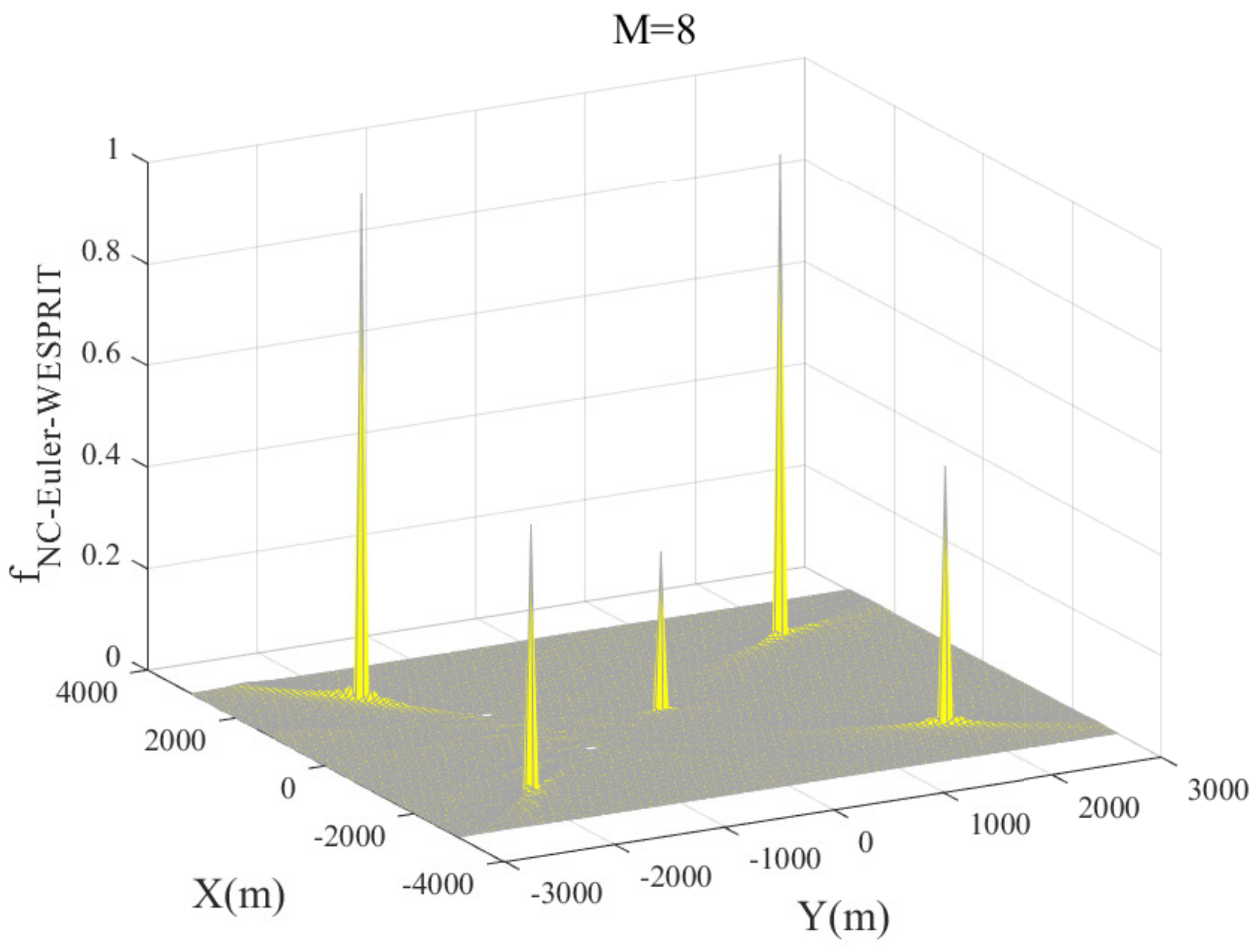
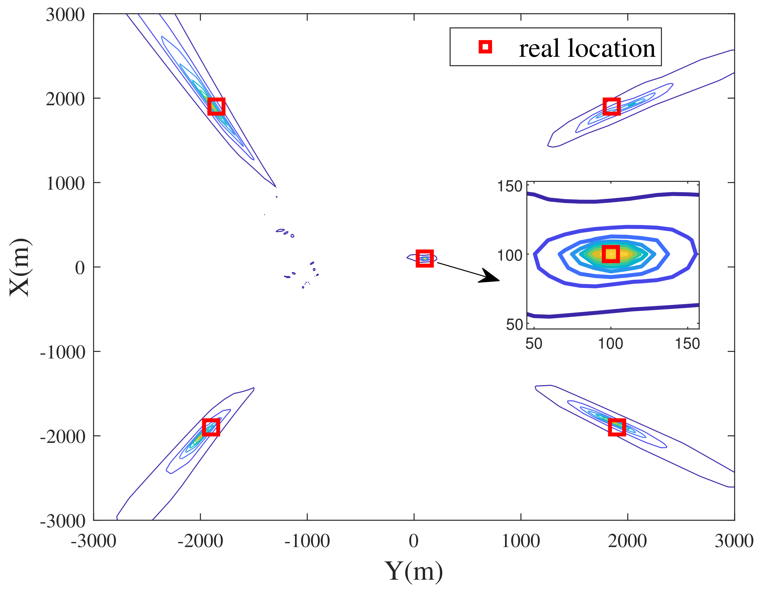
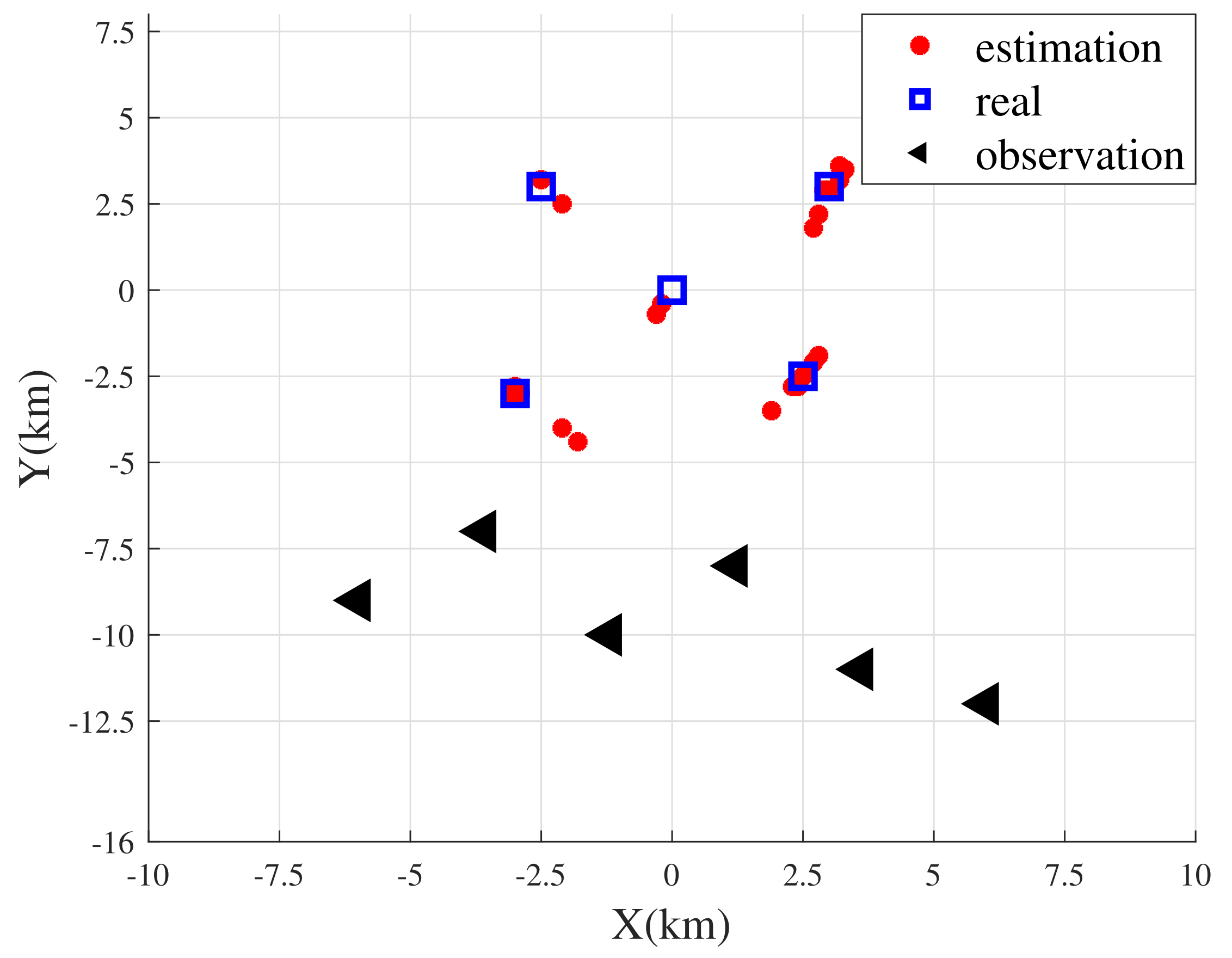
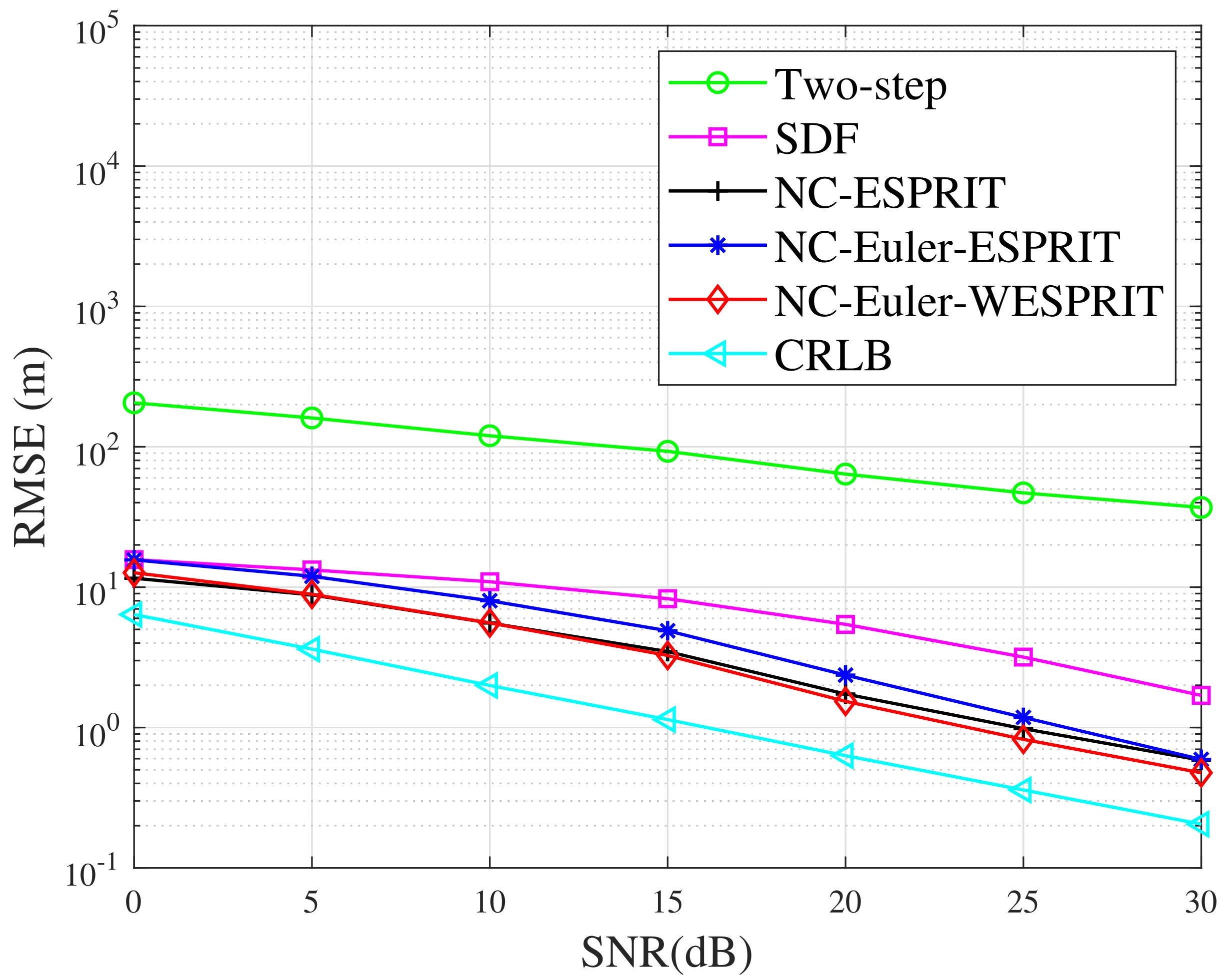
4.4. Simulation Results

To verify the effectiveness of NC-Euler-WESPRIT DPD algorithm, we applied Monte Carlo experiments to evaluate the performance. Define root mean square error (RMSE) as

$$RMSE=\frac{1}{Q}\sum _{q=1}^Q\sqrt{\frac{1}{Mon}\sum _{mn=1}^{Mon}\left[{\left({\widehat{x}}_{q,mn}-x_q\right)}^2+{\left({\widehat{y}}_{q,mn}-y_q\right)}^2\right]},$$

(73)

where $Mon$ represents the number of Monte Carlo experiments and Q stands for the number of targets. $\left({\widehat{x}}_{q,mn},{\widehat{y}}_{q,mn}\right)$ denotes the estimated position of the $q\mathrm{th}$ target in the $mn\mathrm{th}$ experiment, $\left(x_q,y_q\right)$ represents the real position of the $q\mathrm{th}$ target. See

Table 2. Parameters of simulation experiments.

Simulation Parameters	Value	Unit
$SNR$(signal to noise ratio)	0~30	dB
G(number of observation stations)	6	-
Q(number of targets)	5	-
$\lambda$(wavelength)	1	m
d(interval of array elements)	$\lambda /2$	m
M(number of antennas)	6	-
K(number of snapshots)	10~300	-
$Mon$(number of Monte Carlo)	1000	-
${\sigma }_{error}^2$(heteroscedasticity)	10	-
$\mathit{p}$(target locations)	(−3000,−3000) (0,0) (3000,3000)	m
	(−2500,3000) (2500,−2500)
$\mathit{\phi }$(NC phase)	[10,40,30,50,60]	rad
$\mathit{u}$(observation locations)	(−6000,−9000) (−3600,−7000) (−1200,−10,000)	m
	(1200,−8000) (3600,−11,000) (6000,−12,000)

for other simulation parameters. Moreover, to show the heteroscedasticity of the received SNR at each observation station [36], we define

$${\sigma }_{error}^2=\frac{1}{G}\sum _{g=1}^G{\parallel {\alpha }_g-{\overline{\alpha }}_g\parallel }^2,$$

(74)

where

$${\alpha }_g={\left[{\alpha }_{g,1},{\alpha }_{g,2}\cdots ,{\alpha }_{g,Q}\right]}^T\in {\mathbb{R}}^{Q\times 1},$$

(75)

$${\overline{\alpha }}_g=\frac{1}{Q}\sum _{q=1}^Q{\alpha }_{g,q}$$

(76)

$${\overline{\alpha }}_g={\left[{\overline{\alpha }}_g,{\overline{\alpha }}_g,\cdots ,{\overline{\alpha }}_g\right]}^T\in {\mathbb{R}}^{Q\times 1}$$

(77)

Simulation 1: Discuss the performance of NC-Euler-WESPRIT algorithm with different array elements. Considering that five far-field targets impact six observation stations, NC phases and locations of targets are (20, 40, 50, 60, 70) and [(−1900,−1900), (−1850,1900), (100,100), (1850,1900), (1900,−1900)], respectively. ${\sigma }_{error}^2=10$, $K=300$, $SNR=30\mathrm{dB}$ and the observation locations are [(−800,−900), (−480,−700), (−160,−1000), (160,−800), (480,−1100), (800,−1200)]. $M=4$ in Figure 3 and $M=8$ in Figure 4. The spectral peak diagrams show that NC-Euler-WESPRIT algorithm can successfully distinguish the targets even when the number of array elements at each observation station is less than that of targets. Besides, the estimation performance of NC-Euler-WESPRIT algorithm is getting better and better with the increase of the number of array elements.

Simulation 2: Discuss the performance of NC-Euler-WESPRIT algorithm with different snapshots. Considering that five far-field targets impact six observation stations. $SNR=20\mathrm{dB}$, $M=5$. $K=50$ in Figure 5 and $K=300$ in Figure 6. The other simulation parameters are the same as simulation 1. The contour figures indicate that NC-Euler-WESPRIT algorithm can successfully distinguish the targets with small snapshots. In addition, the sidelobe of the spectral peak becomes smaller with the increase of snapshots.

Simulation 3: Discuss the performance of NC-Euler-WESPRIT algorithm with different SNRs. Considering that five far-field targets impact six observation stations. $Mon=5$, $K=200$, ${\sigma }_{error}^2=5$, $M=4$. Other simulation parameters are in Table 2. SNRs in Figure 7 and Figure 8 are 15 dB and 30 dB, respectively. It can be seen from scatter diagrams that NC-Euler-WESPRIT method can distinguish targets at low SNR well. Moreover, the estimation performance of NC-Euler-WESPRIT method is getting better and better with the increase of SNR.

Simulation 4: Discuss the RMSE performance of NC-Euler-WESPRIT algorithm with different ${\sigma }_{error}^2$ varying with SNR. Considering that three far-field targets impact six observation stations. NC phases and locations of targets are (40,50,60) and [(−3000,−3000), (0,0), (3000,3000)], respectively. Other parameters are in Table 2. The ${\sigma }_{error}^2$ in Figure 9 and Figure 10 are 50 and 70, respectively. Other parameters are in Table 2. From the figures, the performance of NC-Euler-WESPRIT method is superior to original two-step positioning method [12], SDF technology [27], NC-ESPRIT and NC-Euler-ESPRIT. Compared with the method before Euler transformation, the estimation performance of NC-Euler-ESPRIT algorithm is closed to it. In addition, the superior performance of NC-Euler-WESPRIT algorithm is more obvious when the heteroscedasticity of the received SNR at each observation station increases.

Simulation 5: Discuss the RMSE performance of NC-Euler-WESPRIT algorithm with different ${\sigma }_{error}^2$ varying with snapshot. Considering that three far-field targets impact six observation stations. NC phases and locations of targets are (40,50,60) and [(−3000,−3000), (0,0), (3000,3000)], respectively. SNR is 15 dB. The ${\sigma }_{error}^2$ in Figure 11 and Figure 12 are 50 and 70, respectively. Other parameters are in Table 2. The figures indicate that the performance of NC-Euler-WESPRIT method is superior to original two-step location method [12], SDF technology [27], NC-ESPRIT and NC-Euler-ESPRIT. Compared with the method before Euler transformation, the estimation performance of NC-Euler-ESPRIT algorithm is closed to it. In addition, the superior performance of the proposed NC-Euler-WESPRIT algorithm is more obvious when the heteroscedasticity of the received SNR at each observation station increases.

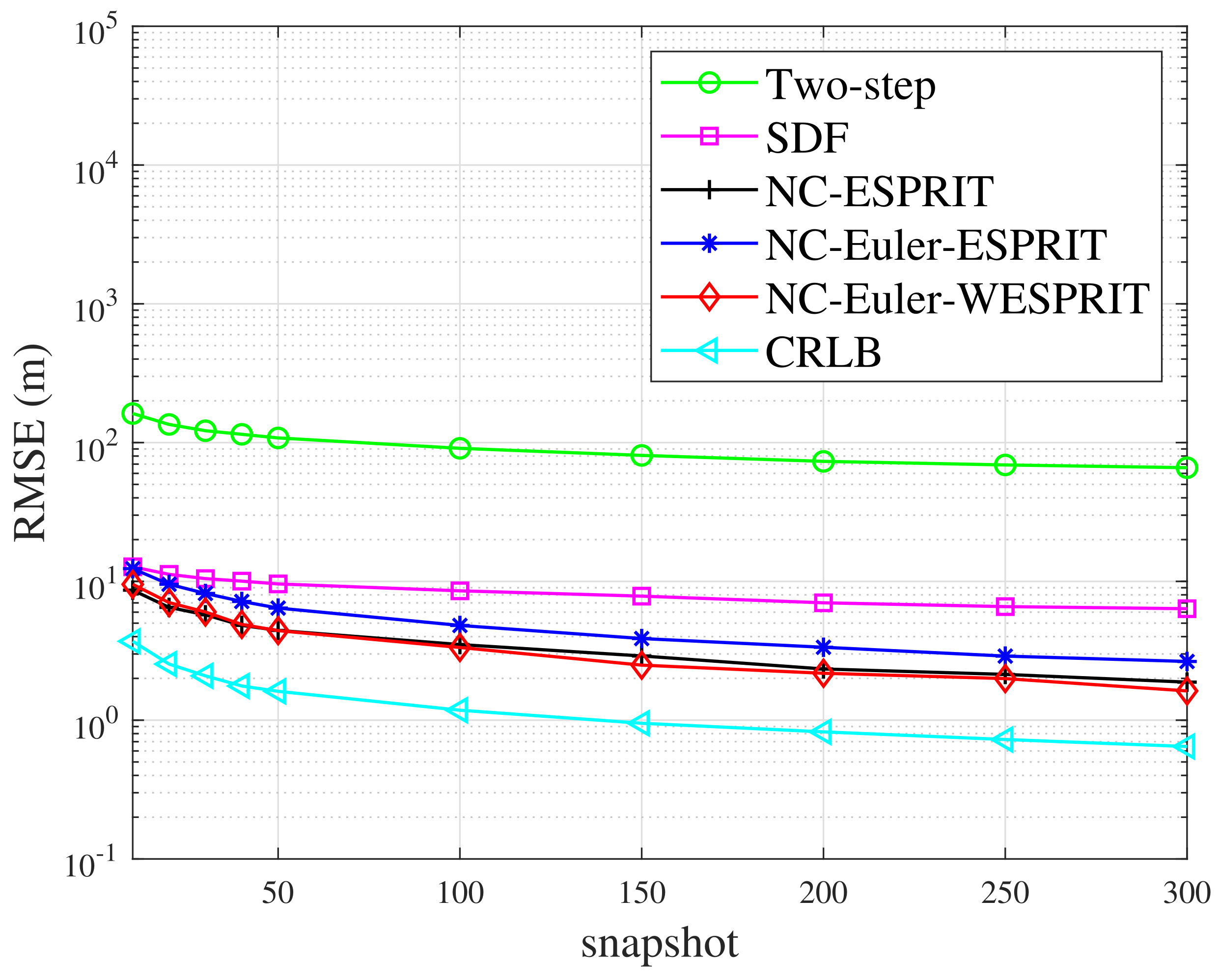
4.5. Advantages of the Proposed Algorithm

The advantages of NC-Euler-WESPRIT algorithm are summarized as follows:

(1)

The proposed NC-Euler-WESPRIT algorithm has more available degrees of freedom than original two-step positioning method, SDF method and can distinguish more targets.

(2)

The proposed NC-Euler-WESPRIT algorithm significantly reduces the computational complexity compared with SDF method and NC-ESPRIT algorithm.

(3)

By weighting the received data of each observation station, the proposed NC-Euler-WESPRIT algorithm has higher positioning precision than original two-step positioning method and SDF method.

5. Conclusions

This paper derives direct position determination of non-circular sources for multiple arrays via weighted Euler ESPRIT data fusion. The proposed NC-Euler-WESPRIT algorithm takes full advantage of elliptic covariance information of NC signals to expand the virtual array aperture. By comparison with original two-step positioning technology and SDF technology, NC-Euler-WESPRIT algorithm has more available DOF. Secondly, this paper introduces the idea of Euler-ESPRIT and constructs a spectral function without complex multiplication. According to the running time of the algorithms, the proposed algorithm greatly reduces the complexity compared with the original SDF algorithm and NC-ESPRIT algorithm. In addition, the proposed algorithm reduces the performance loss caused by signal propagation loss in space as much as possible by weighting the received data of each observation station. Simulation results verify that the proposed NC-Euler-WESPRIT algorithm can effectively estimate the targets even when the number of array elements of each observation station is less than that of targets and its positioning performance is superior to original two-step positioning method and SDF algorithm. While our proposed method only considers the situation of uniform linear array, sparse arrays are now the focus of attention, which is the future work due to the fact that sparse arrays will bring great challenge on the non-circular signals.

References

1. Hameed, K.; Tu, S.; Ahmed, N.; Khan, W.; Armghan, A.; Alenezi, F.; Alnaim, N.; Qamar, M.S.; Basit, A.; Ali, F. DOA Estimation in Low SNR Environment through Coprime Antenna Arrays: An Innovative Approach by Applying Flower Pollination Algorithm. Appl. Sci. 2021, 11, 7985. [Google Scholar] [CrossRef]
2. Ma, F.; Liu, Z.M.; Guo, F. Direct Position Determination in Asynchronous Sensor Networks. IEEE Trans. Veh. Technol. 2019, 68, 8790–8803. [Google Scholar] [CrossRef]
3. Mazuelas, S.; Lorenzo, R.M.; Bahillo, A.; Fernandez, P.; Prieto, J.; Abril, E.J. Topology Assessment Provided by Weighted Barycentric Parameters in Harsh Environment Wireless Location Systems. IEEE Trans. Signal Process. 2010, 58, 3842–3857. [Google Scholar] [CrossRef]
4. Wang, L.; Yang, Y.; Liu, X. A Direct Position Determination Approach for Underwater Acoustic Sensor Networks. IEEE Trans. Veh. Technol. 2020, 69, 13033–13044. [Google Scholar] [CrossRef]
5. Liu, Y.; Wang, C.X.; Huang, J.; Sun, J.; Zhang, W. Novel 3-D nonstationary mmWave massive MIMO channel models for 5G high-speed train wireless communications. IEEE Trans. Veh. Technol. 2018, 68, 2077–2086. [Google Scholar] [CrossRef]
6. Qun, Y.; Yi, Y.; Xiang-yu, C.; Xu, Y. Analysis of DOA and adaptive beam forming including mutual coupling. In Proceedings of the 2011 IEEE International Conference on Signal Processing, Communications and Computing (ICSPCC), Xi’an, China, 14–16 September 2011; pp. 1–4. [Google Scholar] [CrossRef]
7. Bell, K.L.; Pitre, R. MAP-PF 3D position tracking using multiple sensor array. In Proceedings of the 2008 5th IEEE Sensor Array and Multichannel Signal Processing Workshop, Darmstadt, Germany, 21–23 July 2008; pp. 238–242. [Google Scholar] [CrossRef]
8. Chen, P.; Chen, Z.; Cao, Z.; Wang, X. A New Atomic Norm for DOA Estimation with Gain-Phase Errors. IEEE Trans. Signal Process. 2020, 68, 4293–4306. [Google Scholar] [CrossRef]
9. Wang, Y.; Ma, S.; Chen, C.L.P. TOA-Based Passive Localization in Quasi-Synchronous Networks. IEEE Commun. Lett. 2014, 18, 592–595. [Google Scholar] [CrossRef]
10. Qiao, T.; Zhang, Y.; Liu, H. Nonlinear Expectation Maximization Estimator for TDOA Localization. IEEE Wirel. Commun. Lett. 2014, 3, 637–640. [Google Scholar] [CrossRef]
11. Xie, Y.; Wang, Y.; Zhu, P.; You, X. Grid-search-based hybrid TOA/AOA location techniques for NLOS environments. IEEE Commun. Lett. 2009, 13, 254–256. [Google Scholar] [CrossRef]
12. Liu, J.; Lee, J.; Li, L.; Luo, Z.Q.; Wong, K. Online clustering algorithms for radar emitter classification. IEEE Trans. Pattern Anal. Mach. Intell. 2005, 27, 1185–1196. [Google Scholar] [CrossRef]
13. Amar, A.; Weiss, A.J. Direct position determination in the presence of model errors—Known waveforms. Digit. Signal Process. 2006, 16, 52–83. [Google Scholar] [CrossRef]
14. Weiss, A. Direct position determination of narrowband radio frequency transmitters. IEEE Signal Process. Lett. 2004, 11, 513–516. [Google Scholar] [CrossRef]
15. Picinbono, B. On circularity. IEEE Trans. Signal Process. 1994, 42, 3473–3482. [Google Scholar] [CrossRef]
16. Amar, A.; Weiss, A.J. Direct position determination (DPD) of multiple known and unknown radio-frequency signals. In Proceedings of the 2004 12th European Signal Processing Conference, Vienna, Austria, 6–10 September 2004; pp. 1115–1118. [Google Scholar]
17. Bar-Shalom, O.; Weiss, A.J. Direct position determination of OFDM signals. In Proceedings of the 2007 IEEE 8th Workshop on Signal Processing Advances in Wireless Communications, Helsinki, Finland, 17–20 June 2007; pp. 1–5. [Google Scholar] [CrossRef]
18. Oispuu, M.; Nickel, U. Direct detection and position determination of multiple sources with intermittent emission. Signal Process. 2010, 90, 3056–3064. [Google Scholar] [CrossRef]
19. Qin, T.; Li, L.; Lu, Z.; Wang, D. A ML-Based Direct Localization Method for Multiple Sources with Moving Arrays. In Proceedings of the 2018 IEEE 18th International Conference on Communication Technology (ICCT), Chongqing, China, 8–11 October 2018; pp. 1073–1076. [Google Scholar] [CrossRef]
20. Zhou, T.; Yi, W.; Kong, L. Direct position determination of multiple coherent sources using an iterative adaptive approach. Signal Process. 2019, 161, 203–213. [Google Scholar] [CrossRef]
21. Zhang, X.; Wang, Q.; Huang, Z.; Yuan, N.; Hu, W. Direct Position Determination of Emitters using Single Moving Coprime Array. In Proceedings of the 2021 14th International Congress on Image and Signal Processing, BioMedical Engineering and Informatics (CISP-BMEI), Shanghai, China, 23–25 October 2021; pp. 1–5. [Google Scholar] [CrossRef]
22. Xin Yin, J.; Wu, Y.; Wang, D. Direct Position Determination of Multiple Noncircular Sources with a Moving Array. Circuits Syst. Signal Process. 2017, 36, 4050–4076. [Google Scholar] [CrossRef]
23. Yin, J.; Wang, D.; Wu, Y.; Yao, X. ML-based single-step estimation of the locations of strictly noncircular sources. Digit. Signal Process. 2017, 69, 224–236. [Google Scholar] [CrossRef]
24. Yin, J.; Wang, D.; Wu, Y. An Efficient Direct Position Determination Method for Multiple Strictly Noncircular Sources. Sensors 2018, 18, 324. [Google Scholar] [CrossRef] [Green Version]
25. Zhang, Y.K.; Xu, H.Y.; Ba, B.; Wang, D.M.; Geng, W. Direct Position Determination of Non-Circular Sources Based on a Doppler-Extended Aperture with a Moving Coprime Array. IEEE Access 2018, 6, 61014–61021. [Google Scholar] [CrossRef]
26. Qin, T.; Lu, Z.; Ba, B.; Wang, D. A Decoupled Direct Positioning Algorithm for Strictly Noncircular Sources Based on Doppler Shifts and Angle of Arrival. IEEE Access 2018, 6, 34449–34461. [Google Scholar] [CrossRef]
27. Zhang, Y.; Ba, B.; Wang, D.; Geng, W.; Xu, H. Direct Position Determination of Multiple Non-Circular Sources with a Moving Coprime Array. Sensors 2018, 18, 1479. [Google Scholar] [CrossRef] [PubMed] [Green Version]
28. Li, J.; He, Y.; Zhang, X.; Wu, Q. Simultaneous Localization of Multiple Unknown Emitters Based on UAV Monitoring Big Data. IEEE Trans. Ind. Inform. 2021, 17, 6303–6313. [Google Scholar] [CrossRef]
29. Haardt, M.; Romer, F. Enhancements of unitary ESPRIT for non-circular sources. In Proceedings of the 2004 IEEE International Conference on Acoustics, Speech, and Signal Processing, Montreal, QC, Canada, 17–21 May 2004; Volume 2, pp. 101–104. [Google Scholar]
30. Viswanath, P.; Tse, D.; Anantharam, V. Asymptotically optimal water-filling in vector multiple-access channels. IEEE Trans. Inf. Theory 2001, 47, 241–267. [Google Scholar] [CrossRef]
31. Petrus, P.; Ertel, R.; Reed, J. Capacity enhancement using adaptive arrays in an AMPS system. IEEE Trans. Veh. Technol. 1998, 47, 717–727. [Google Scholar] [CrossRef]
32. Jeng, S.S.; Xu, G.; Lin, H.P.; Vogel, W. Experimental studies of spatial signature variation at 900 MHz for smart antenna systems. IEEE Trans. Antennas Propag. 1998, 46, 953–962. [Google Scholar] [CrossRef]
33. Qian, Y.; Yang, Z.; Zeng, H. Direct Position Determination for Augmented Coprime Arrays via Weighted Subspace Data Fusion Method. Math. Probl. Eng. 2021, 2021, 1–10. [Google Scholar] [CrossRef]
34. Kumar, G.; Ponnusamy, P.; Amiri, I.S. Direct Localization of Multiple Noncircular Sources with a Moving Nested Array. IEEE Access 2019, 7, 101106–101116. [Google Scholar] [CrossRef]
35. Stoica, P.; Arye, N. MUSIC, maximum likelihood, and Cramer-Rao bound. IEEE Trans. Acoust. Speech Signal Process. 1989, 37, 720–741. [Google Scholar] [CrossRef]
36. Shi, X.; Zhang, X. Weighted Direct Position Determination via the Dimension Reduction Method for Noncircular Signals. Math. Probl. Eng. 2021, 2021, 1–10. [Google Scholar] [CrossRef]
Figure 1. Scene of multiple arrays positioning.
Applsci 12 02503 g001
Figure 2. The running time of different algorithms varying with search grids.
Applsci 12 02503 g002
Figure 3. Cost function of NC-Euler-WESPRIT ( M = 4 ).
Applsci 12 02503 g003
Figure 4. Cost function of NC-Euler-WESPRIT ( M = 8 ).
Applsci 12 02503 g004
Figure 5. Contour diagram of NC-Euler-WESPRIT ( K = 50 ).
Applsci 12 02503 g005
Figure 6. Contour diagram of NC-Euler-WESPRIT ( K = 300 ).
Applsci 12 02503 g006
Figure 7. Scatter diagram of NC-Euler-WESPRIT ( S N R = 15 dB ).
Applsci 12 02503 g007
Figure 8. Scatter diagram of NC-Euler-WESPRIT ( S N R = 30 dB ).
Applsci 12 02503 g008
Figure 9. RMSE performance varying with SNR ( K = 100 , σ e r r o r 2 = 50 ).
Applsci 12 02503 g009
Figure 10. RMSE performance varying with SNR ( K = 100 , σ e r r o r 2 = 70 ).
Applsci 12 02503 g010
Figure 11. RMSE performance varying with snapshot ( S N R = 15 dB , σ e r r o r 2 = 50 ).
Applsci 12 02503 g011
Figure 12. RMSE performance varying with snapshot ( S N R = 15 dB , σ e r r o r 2 = 70 ).
Applsci 12 02503 g012