Abstract
In this study, we examined the robust super-twisting sliding mode backstepping control (SBSC) method, which employed a tracking differentiator and nonlinear disturbance observer for a hexacopter unmanned aerial vehicle (UAV) system. To realize robust tracking control performance for a highly coupled nonlinear hexacopter UAV system, a super-twisting sliding mode control method was combined with designing stabilizing controls of backstepping control (BSC) applied to the UAV system. Furthermore, the differentiation issue of the virtual control and compensation of transformation error in the conventional BSC design were bypassed via a new continuous tracking differentiator structure. Additionally, a new disturbance observer based on the proposed tracking differentiator was considered to estimate uncertainties of the hexacopter UAV. Comparative simulation results demonstrated that the proposed tracking-differentiator-based SBSC scheme (PTSBSC) blended with the tracking differentiator and nonlinear disturbance observer exhibits improved performance when compared to that of conventional BSC and disturbance observer systems.
1. Introduction
Developments of the rechargeable battery source, brushless DC motor, and various related techniques lead to increased research unmanned aerial vehicles (UAVs). The multi-rotor UAVs exhibit significant advantages in terms of hovering capability and maneuverability involving side and backward movement, vertical take-off and landing in 3D space, and lower maintenance cost than other small aerial vehicles [1,2,3,4]. Thus, UAVs were initially used for military applications. However, recently, its applications were extended to agriculture, aerial photography, inspection, surveillance, rescue, transport monitoring, and exploration of inaccessible areas. Most multi-rotor UAVs adopted a four-rotor mounted quadrotor structure, and they exhibit limited power for heavy cargo delivery. Currently, UAVs mounted with more rotors, such as hexacopter and octocopter UAVs, when compared to four rotors, were developed to enforce lifting and higher capabilities in terms of flying time [5,6,7,8,9,10]. When considering the efficiency of UAVs, the hexacopter is more feasible than the octocopter because an increase in the number of rotors leads to an increase in size and cost.
However, safe and reliable flight of multi-rotor UAVs should be secured. This is because severe damages can result if the UAV falls or crashes, and the increased speed rotation of a multi-rotor can lead to more severe accidents. Thus, to guarantee safety and reliability in the flight of multi-rotor UAVs, an effective and robust controller is required to overcome the following challenges: (1) under-actuated control scheme for six degrees of freedom (DOF) with four control inputs; (2) strongly coupled nonlinear dynamics between translational and rotational subsystems and kinematic coupling terms; and (3) uncertainties including external disturbances, such as wind and rain, in outdoor environment and unknown dynamics due to varying load.
Several control methods have been utilized to handle the above issues. Linear control schemes, including proportional-integral-derivative (PID) [7,9,11], linear quadratic regulator (LQR) [12,13], predictive control [14], and control [15] have been initially applied for the fundamental flight task of the multi-rotor UAVs. However, these methods undergo their application limits due to performance degradation when the UAV leaves away its designed trimming points or accepts excessive perturbations. To handle these limits, recursive backstepping control (BSC) [6,16,17] is generally utilized as a baseline controller because BSC is appropriate for the aforementioned coupled higher order nonlinear systems and especially for multi-rotor UAVs [18,19,20,21,22,23]. The procedures for stabilizing system states are recursively repeated in the BSC design by utilizing virtual controllers, and the final controller is obtained in the last recursive step. Thus, a controller for any nonlinear system can be systematically designed without utilizing any linearization, which neglects useful nonlinearities.
Conversely, despite the popularity and advantage of the BSC scheme, there exist several disadvantages in the traditional BSC scheme. First, the virtual stabilizing controls contain the repeated differentiation terms with respect to virtual controls designed during the pre-recursive steps for high-order nonlinear systems. Hence, this leads to an increase in complexity. The tracking differentiator methods [24,25,26,27,28,29,30] were recently investigated as a potential solution. Furthermore, the second-order finite-time command filter [31,32,33] was considered to obtain improved properties to guarantee finite-time convergence and avoid increases in complexity, given that the traditional BSC schemes were designed in the point of infinite-time convergence. However, the traditional tracking differentiators exhibit the disadvantage of slow convergence time, though the recently developed tracking differentiators in [27,28,29] show more improved performance than those of the previous ones.
Second, most BSC systems were designed to be based on the nonlinear model dynamics in each recursive step and are then exposed to the uncertainty issue. Hence, they are sensitive to uncertainties, and control performances will be degraded when the parametric perturbations and external disturbances occur. Further efforts have been made to enforce robustness to uncertainty in the ordinary BSC system.
The first solution for the second issue is that BSC is typically combined with the first-order sliding mode control (SMC) [34] by utilizing the robustness property of SMC. However, there is a chattering disadvantage of the first order SMC [35,36,37,38].
As the second solution for the second issue, to enforce control performance by estimating and compensating uncertainties, several disturbance observers are developed [39,40,41,42,43,44,45]. A disturbance observer studied in [39,40] is applied to estimate uncertainties for nonlinear systems. However, it has the drawback that the observer is designed under the assumption of slow variation of uncertainties. An extended state observer (ESO) in [41,42] is developed on the position feedback, which is commonly obtained by integrating the velocity information of the system, especially for the multi-rotor UAVs. The long-time integration errors will influence the position information, which further degrade estimation accuracy of the observers. Disturbance observers utilizing a tracking differentiator to bypass the differentiation error in velocity feedback routine are developed in [43,44,45]. However, the convergence rate of the state of observer is slow, and the resulting estimation performance for uncertainties is degraded. Hence, to cope with the lower convergence performance in these observers, a more enhanced observer is required to achieve higher estimation and compensation of the uncertainties.
Motivated by the aforementioned works, as an alternative to the first-order SMC, the super-twisting algorithm (STA) [46,47,48,49] was developed because the STA offers the following advantages: it requires only the information on the sliding variable; it provides finite-time convergence to the origin for the sliding variable and its derivative; and it generates a continuous control signal to consequently adjust chattering. Furthermore, a novel continuous tracking differentiator based on the sine hyperbolic function is proposed to enhance lower performance traditional tracking differentiators. Finally, a novel disturbance observer based on the proposed tracking differentiator is examined to estimate the external disturbance in USVs. Therefore, in this study, a BSC system combined with STA (SBSC) is considered to realize finite-time convergence and robustness with respect to uncertainty over the conventional BSC system.
The contributions of this study are summarized as follows:
- (1)
- The traditional BSC is combined with the STA to enforce insensitivity to variation of uncertainties of a hexacopter UAV system and bypass chattering in the traditional BSC combined with the first-order sliding mode control.
- (2)
- The proposed SBSC control strategy for a hexacopter UAV improves finite settling-time convergence when compared to the traditional BSC system. Faster movements of a hexacopter UAV will be expected for a perturbed environmental situation.
- (3)
- A novel continuous tracking differentiator based on the sine hyperbolic function is developed to obtain enhanced convergence of the state variable of the tracking differentiator. Thus, faster output of the command filter approximation on the derivative of the virtual control at each recursive step is acquired. The proposed tracking differentiator system exhibits improved performance when compared to the conventional system.
- (4)
- An improved nonlinear disturbance observer can be designed by utilizing the proposed tracking differentiator. Hence, the performance of estimation and disturbance rejection for uncertainties of the hexacopter UAV control system are improved by utilizing the proposed disturbance observer.
Finally, the performance of the proposed control scheme is evaluated via sequential comparative simulation of a nonlinear hexacopter UAV system.
The rest of the paper is organized as follows. The nonlinear system model of UAV and tracking differentiator are presented in Section 2, and the design process for a SBSC is described in Section 3. Furthermore, stability analysis is discussed in Section 4, and simulation results for a hexacopter UAV system are provided in Section 5. Finally, the summary and conclusion of the study are presented in Section 6.
2. Preliminaries
2.1. UAV Dynamics and Problem Formulation
A hexacopter UAV has a mechanism for generating the required forces and torques. The nonlinear dynamics of a hexacopter, as presented in Figure 1 [10], is expressed as follows:
where denotes position with respect to the inertia frame, denotes Euler angles, and denote linear and angular velocities, respectively, in the body-fixed frame. denotes a symmetric positive definite moment of inertia matrix, ; denotes the resultant torque due to the gyroscopic effect, and and denote uncertainties, including parameter change, asymmetric structure, payload variation, rotor fluctuation, and aerodynamic drag, which are denoted as , , and . denotes the moment of inertia of each rotor and , and denotes the speed of rotor i. The translation force contains gravity, main thrust force, and other force components. The airframe orientation in space is provided using a rotation matrix from the body frame to the navigation frame, and is expressed as follows:
where and denote and , respectively. The lift force and torque are generated by rotors with respect to body-fixed frame as follows:
where denotes the force generated in the i-th rotor, and denote coefficients of drag and thrust of the propeller, respectively, and denotes the distance from rotors to the center of mass. Given the perturbation of the mass of the body due to the loading of the carrying object, (1) is expressed as follows:
where and denotes a mass perturbation. Based on the above results, the translational dynamics equations of the hexacopter can be expressed as follows:
where , , and . Next, the rotational dynamic equations are expressed as follows:
where , , and .
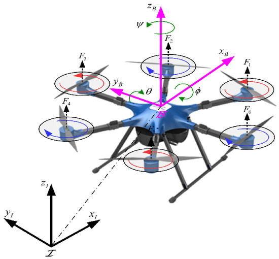
Figure 1.
Description of the hexacopter UAV.
2.2. Tracking Differentiator
In this section, a tracking differentiator is considered to avoid the differentiation of the virtual controls in the BSC scheme.
Theorem 1
([26]). If any solution of the following system:
satisfies , as , then for an arbitrary bounded and integrable input function and a constant , the solution of the following system
satisfies if the solutions of (14) satisfy and as .
Theorem 2
([26]). Consider the following system
The system (15) is global uniformly asymptotically stable if and , are satisfied.
Theorem 3.
Consider the following system
where , , , and are constants. For an arbitrary bounded and integrable function and a constant , can be obtained if the positive conditions of all parameters are satisfied.
Proof.
Transforming and in (16), it follows that because is an odd function. Then, , where means an introduced integral variable. Thus, we can consider the following Lyapunov function:
Taking the time derivative of (17) and using (16) result in
Thus, it is sure that only when . Based on (16), when , will always be equivalent to zero. If and , we obtain that . Hence, the solutions of do not include any other whole trajectory, except the origin (0,0).
Therefore, the system (16) is globally asymptotically stable. This concludes the proof. □
For comparison of the above differentiators, three tracking differentiators were selected. The first one, which is proposed by Yang et al. [27], is the following hyperbolic tangent tracking differentiator:
where . The second one, which was proposed by Zong et al. [28,29], is the tangent sigmoid function tracking differentiator given by
where is a constant. The third one, the first-order sliding mode tracking differentiator proposed by Levant [30,31], is considered, which is described as
3. Design of Controller and Nonlinear Disturbance Observer
3.1. Design of Altitude Controller
The vertical displacement is determined by the altitude controller. The state equation for altitude dynamics in (8) can be expressed as follows:
where the altitude state variable , , and . By introducing the command trajectory in the z-coordinate, the sliding mode surfaces to include the tracking error and new states are defined as follows:
where the sliding mode surfaces include the tracking error and the compensating signals. The state variables and in (23) and (24) are obtained from the dynamics of the compensating signals expressed as follows:
where , denote constants. Next, the output of the tracking differentiator is obtained from the tracking differentiator dynamics described in Theorem (3):
where , , . denotes the virtual control defined later, and are constants, and and denote constants. We define the following super-twisting state variable vectors to design the controller using the variables defined previously.
The super-twisting state variable vectors consist of the sliding mode surfaces and signum functions. Using the definition in (23), the time derivative of the components of the state vectors in (27) and (28) can then be written as
where and . We can select the virtual control from (29) and control input from (31) as follows:
where , and , , are constants, the virtual control input denotes the recursive input, and denotes the final control input. Using (33) and (34), (29) and (31) can be expressed as follows:
where denotes the estimate error. Considering the above results, the following compact expressions can be obtained:
We define the Lyapunov function candidate as follows:
where denotes positive definite matrices defined as follows:
Differentiating (39) with respect to time and using (37) and (38) result in the following expression:
where , , and the positive definite matrix
3.2. Design of Longitudinal and Latitudinal Controllers
Let us define the state variables for x-, y-axes and roll, pitch axes from (6), (7), (9), and (10) as , , , and . The state–space model is represented as follows:
where , , , , , and , . We define the sliding mode vectors including the tracking command, errors, and state variables as
In the sliding mode surfaces, the dynamics of the compensating signals , , is described as
where , are constants. Furthermore, is obtained from the tracking differentiator described as follows:
where , , and are constants. We define the following super-twisting state variable vectors to design the controller using the variables defined previously
The differentiation of the above state vectors is as follows:
where . We can select the virtual controls for the recursive input, and control inputs as follows:
where , , and , are constants. Next, substituting these controls into the dynamics of the compensating signals given in (47) and repeating the procedures of the previous step, we obtain the following compact expressions for the super-twisting state vector:
where , . The Lyapunov function candidate with (60) and (61) is defined as follows:
where denotes positive definite matrices defined as follows:
The time derivative of (63) leads to the following expression:
where , and the positive definite matrix
3.3. Design of the Heading Controller
Let us define the state variable for the yaw axis from (11) as and . Hence, the state–space model can be represented as follows:
where , , and . The tracking error and new states are defined as follows:
The compensating signals included in (66) and (67) are obtained from the following dynamics:
where are constants. In (67), denotes the output of the tracking differentiator expressed as follows:
where , , and are constants. The super-twisting state variable vectors are defined as
Next, the time derivatives of the state vector to design the controllers are given by
where and . We can select the virtual control for recursive input and control input as follows:
We define the Lyapunov function candidate as follows:
where denotes positive definite matrices defined with and as follows:
Substituting (74) and (75) into (72) and (73), respectively, and differentiating (76) with respect to time results in the following expression:
where , , and the positive definite matrix
3.4. Design of the Disturbance Observer
Assumption 1.
The disturbance is bounded such that there exists an unknown constant that satisfies .
Theorem 4.
The disturbances are estimated by the following novel nonlinear disturbance observers:
where denotes the state vector, including the super-twisting state vector, denotes the state vector of the tracking differentiator, denotes the state vector of the compensating signal, , , , , and denote the estimates of and , , and are diagonal positive constant matrices, respectively. Evidently, and when .
Proof.
When , can be assumed as an infinitely large value. This indicates that the variation in significantly exceeds . Furthermore, it suggests that , . Hence, it is easy to note that (78) holds according to Theorem (1) when is considered as . This concludes the proof. □
To compare of the proposed observer with the conventional observers, two disturbance observers were provided. The first observer is designed using the structure of the tracking differentiator proposed by Zong et al. [28,29] expressed in (20) as follows:
The second observer is designed using the structure of the tracking differentiators proposed by Levant [30,31] expressed in (21) as follows:
4. Stability Analysis
Lemma 1.
([50]). Consider the system . For the given positive scalar constants, , , , and , if the continuous function satisfies , then the trajectory of the system is finite time stable and convergence time is bounded as follows:
Theorem 5.
If the sliding mode surfaces are defined as (23), (24), (43)–(46), (66), and (67), then systems (7)–(12) are controlled by virtual controls (33), (57), (58), (74) and control inputs (34), (59), (60), (75), and the unknown disturbances are estimated by the nonlinear disturbance observer provided in (78). Furthermore, the equilibrium points of (7)–(12) are asymptotically stable, and the trajectory of the closed-loop signals is bounded in finite time as follows:
if the parameter conditions guarantee positive definiteness of , i.e.,
Proof.
By defining the Lyapunov function as using the results from (39), (63), and (76), we can obtain the following expression:
Given that
and , and , then
where , , , and . Then, (74) is expressed as follows:
or
given that , we obtain the following expression:
From Lemma 1, the boundedness of decreases argument
Thus, the convergence time is given as follows:
Next, given that , we obtain the following expression:
This leads to the following:
Therefore, is a continuously decreasing strong Lyapunov function, and the equilibrium point is reached in finite time from every initial condition. This also guarantees that the equilibrium point is reached in finite time from every initial condition. This concludes the proof. □
Theorem 6.
The finite time convergence of the compensating dynamics given in (25), (47), and (68) is also guaranteed by the finite time convergence of . Thus, the finite time boundedness of is demonstrated by defining the following expression:
The convergence time is then obtained as
Proof.
From (96), one can obtain that
where and can be achieved in finite time. Then, (98) is expressed under the condition of as
with . Then, (99) is expressed as follows:
under the condition that there exists a scalar . If is satisfied, (100) is expressed as follows:
Consequently, approaches zero in finite time, and the finite time convergence of is guaranteed. The convergence time is obtained as follows:
This concludes the proof. □
5. Simulation Results
In this section, simulations for three cases, including the nominal system, perturbed system without the observer, and perturbed system with the observer are conducted to evaluate the performance of the proposed controller and disturbance observer for the hexacopter UAV system. Four control systems were designed to compare the proposed scheme with the conventional methods: namely, the standard BSC system (BSC); Levant’s tracking differentiator [31,32] based BSC system (YTBSC) studied by Yu et al. [50]; Zong’s tracking differentiator [28,29] based BSC system (ZTBSC), where the adopted controller is designed according to those in [50]; and proposed tracking differentiator and super-twisting algorithm based BSC system (PTSBSC). The system parameters of the hexacopter UAV are listed in Table 1 of [10].

Table 1.
Selected values of the hexacopter UAV.
To compare the performance of the tracking differentiators presented in Section 2, the parameters are selected as , , and under the initial condition of , , and . Comparative results are presented in Figure 2, where the proposed differentiator shows more rapid convergence performance than others. Only three tracking differentiators are considered, excluding the tracking differentiator proposed by Yang et al. [27] due to its lower performance.
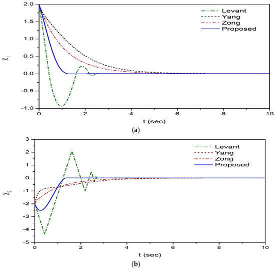
Figure 2.
Comparative results for three tracking differentiators. (a) . (b) .
5.1. Simulation Results of the Nominal Hexacopter USV System
The design parameters of the controller and observer are selected via the trial-and-error method. The selected values are listed in Table 2, Table 3 and Table 4.
Table 2.
Selected values of the tracking differentiator.
Table 3.
Selected values of the compensating signal.
Table 4.
Selected values of the disturbance observer.
The command trajectories of each axis were selected as follows:
Simulation results for the nominal hexacopter system are shown in Figure 3, wherein the additional load mass and disturbances are not considered. The position tracking result in 3D space is shown in Figure 3a. The position tracking results for the translation axes are presented in Figure 3b–d. The angular position tracking results are shown in Figure 3e–g. To clarify the tracking performance for each control system, tracking errors for x, y, z, and axes are shown in Figure 3i–l. As shown in Figure 3i,j, the tracking performances of the BSC and YTBSC are similar. As shown in Figure 3k, the improvement in the tracking performance of the z-axis of the YTBSC exceeds that of the BSC system. However, the performance of the PTSBSC system exceeds that of the other two systems as shown in Figure 3h–k. The control inputs of the altitude and heading controllers are shown in Figure 3l,m, respectively.
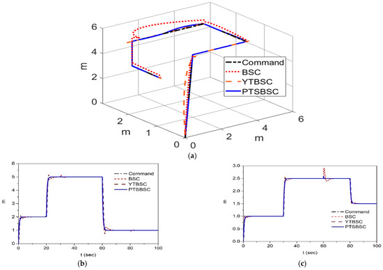
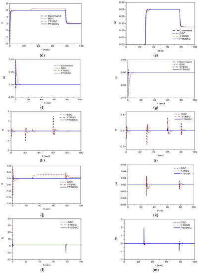
Figure 3.
Simulation results of the nominal hexacopter system. (a) The 3D tracking result. (b) Output of x-axis. (c) Output of y-axis. (d) Output of z-axis. (e) Output of -axis. (f) Output of -axis. (g) Output of -axis. (h) Tracking error of x-axis. (i) Tracking error of y-axis. (j) Tracking error of z-axis. (k) Tracking error of -axis. (l) Control input of latitude controller. (m) Control input of heading controller.
5.2. Simulation Results of the Perturbed System
Subsequently, simulation for the perturbed system with a 200% increase in the mass of the hexacopter, which denotes the variation in the load mass, is conducted to evaluate robustness with respect to the load perturbation. The other perturbations are as follows:
Additionally, the wind disturbance of is applied to the x-axis. The simulation results are shown in Figure 4, where the 3D tracking result is shown in Figure 4a and the tracking results in each axis are shown in Figure 4b–e. Outputs in the x and y axes of the conventional BSC system indicate high oscillation, and the latitude error exceeds those of other systems. The outputs of the YTBSC system exhibit high overshoot in the point of direction change as shown in Figure 4b–e. Conversely, the simulation results in Figure 4 indicate that the robustness of the proposed PTSBSC system exceeds those of the two systems for the disturbance due to mass variation and other disturbances.
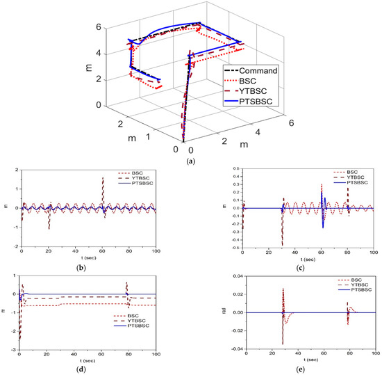
Figure 4.
Simulation results of the perturbed hexacopter system. (a) 3D tracking result. (b) Tracking error for x-axis. (c) Tracking error for y-axis. (d) Tracking error for z-axis. (e) Tracking error for -axis.
5.3. Simulation Results of the Perturbed System with Disturbance Observer
Under the same disturbance conditions, as listed in Section 5.2, simulation for the perturbed system with the controller blended with the disturbance observers based on (78) (proposed), (79) (Zong [28,29]), and (80) (Levant [30,31]) is conducted to evaluate the estimation performance. The simulation results are shown in Figure 5, where the 3D tracking result is presented in Figure 4a and the tracking errors in the x, y, z, and -axes are shown in Figure 5b–e. The results indicate that the tracking results of the control system with the proposed observer exhibit a more efficient performance than that of the controller with the Levant observer. The estimates of the observer states and disturbances of the proposed observer are shown in Figure 5f–i. Estimates of the observer states and disturbances of the Levant observer are shown in Figure 5j–m. Finally, estimates of the observer states and disturbances of the Levant observer are shown in Figure 5n–q. The simulation results indicate that the estimate performance of the proposed observer exceeds that of the conventional Levant and Zong observers. Table 5 shows the root mean square (RMS) value of the tracking error of each system, where it is shown that the RMS value of the proposed system decreases until an average 7% of that of Levant’s system.
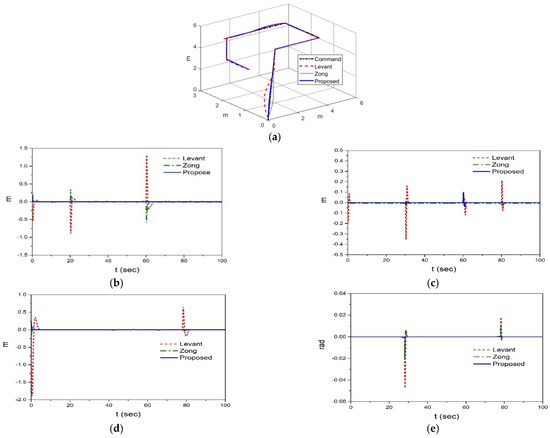
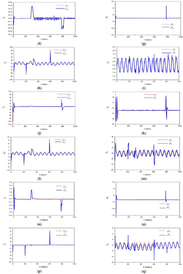
Figure 5.
Simulation results of the perturbed hexacopter system with the controller combined with the disturbance observer. (a) The 3D tracking result. (b) Tracking error for x-axis. (c) Tracking error for y-axis. (d) Tracking error for z-axis. (e) Tracking error for -axis. (f) and of the proposed observer. (g) and of the proposed observer. (h) and of the proposed observer. (i) and of the proposed observer. (j) and of the Levant observer. (k) and of the Levant observer. (l) and of the Levant observer. (m) and of the Levant observer. (n) and of the Zong observer. (o) and of the Zong observer. (p) and of the Zong observer. (q) and of the Zong observer.
Table 5.
RMS value of the tracking error of each system.
Finally, under the disturbance condition with the 300% increase in the mass and the same other condition, simulation for the perturbed system is conducted to evaluate the estimation performance with the disturbance observers based on (78) (proposed), (79) (Zong [28,29]), and (80) (Levant [30,31]). The desired 8-shape command trajectory is described as
under other rotation commands set to be zero value.
In the first stage, the hexacopter UAV climbs vertically for 4 s to simulate the take-off flight. Next, it follows an 8-shaped path while continuing to lift. In the second stage, the lift, sideslip, and forward performances of the hexacopter UAV are evaluated comprehensively. The simulation results are shown in Figure 6, where the 3D tracking result is presented in Figure 6a, and the tracking output and errors in the x, y, z axes are shown in Figure 6b–g. The simulation results indicate that the tracking results of the control system with the proposed observer exhibit a more efficient performance than that of the controller with the Levant observer, like the previous results. Table 6 shows the root mean square (RMS) value of the tracking error of each system, where it is shown that the RMS value of the proposed system decreases until an average 27% of that of Levant’s system.
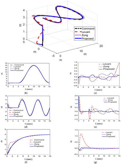
Figure 6.
Simulation results of the perturbed hexacopter system for 300% increase in the mass with the controller combined with the disturbance observer. (a) The 3D tracking result. (b) Output of x-axis. (c) Tracking error of x-axis. (d) Output of y-axis. (e) Tracking error of y-axis. (f) Output of z-axis. (g) Tracking error of z-axis.
Table 6.
RMS value of the tracking error of each system.
5.4. Discussions
Simulations are conducted for three cases, such as nominal system, perturbed system without disturbance observers, and perturbed system with disturbance observers. Simulation results of the nominal system for the linear position command trajectory show that the performance of the PTSBSC system exceeds that of the other BSC and YTBSC systems. This achievement is obtained, owing to the improved performance of the proposed tracking differentiator. The proposed tracking differentiator shows the best performance over the conventional tracking differentiators, including the recently developed ones.
The second simulation under the condition of the perturbation with wind gust and 200% increase in the mass is conducted to the control system without the disturbance observer. In this case, the control performance is only dependent on the property of the controller itself. The proposed PTSBSC system maintains the least performance variation compared with other two BSC and YTBSC systems, where a large variation of the output tracking results appears.
Finally, the disturbance observers are utilized to estimate uncertainties, such as the wind gust and 200% and 300% variations in the mass. Simulations are conducted for the linear position and 8-shaped command trajectories to evaluate various aspects of the control performance. The output performances are determined by the superiority of the adopted observer, where the proposed disturbance observer shows the outperforming estimation results. Therefore, the proposed control system with the novel disturbance observer is ascertained to provide the outperforming results compared to those of the traditional similar controller and disturbance observer systems.
In addition, the phenomenon of pilot-induced oscillations (PIOs) that represent a particular and specific aspect of the framework of human–machine interactions was and still is a dynamic behavior of great interest in the design of aircraft [51]. PIOs consists of sustained or uncontrollable oscillations, resulting from efforts of the pilot to control the aircraft. The disturbance problem of PIOs can occur also in controlling UAVs. However, the possibility to exploit strategies from nonlinear dynamics for controlling PIOs took fewer attention in the UAV control system. In this study, this type of disturbance was not considered yet. As a further study including an experimental examination, it is worth to explore this disturbance by the proposed nonlinear controller and disturbance observer to seek a more feasible control system under various aspects of real flight conditions of UAVs.
6. Conclusions
In this study, a super-twisting sliding mode backstepping control blended with a new tracking differentiator and disturbance observer based on the concept of the proposed tracking differentiator was examined to realize robust tracking control performance of a hexacopter UAV system. Recursive design in conventional backstepping control and faster convergence enabled the improved tracking differentiator to bypass the occurred repeated differentiation issue and obtain the continuous and smooth derivative of the virtual control. Next, the enhanced disturbance observer was designed to estimate uncertainties of the hexacopter UAV system based on the proposed tracking differentiator. Thus, the robust nonlinear controller equipped with the improved disturbance observer was designed to obtain a hexacopter UAV control system that outperforms the conventional control scheme in conditions with high nonlinearities and unknown disturbances. Sequential comparative simulations for the hexacopter nonlinear UAV system in a nominal case and a case with variation in the load mass and wind disturbance were executed, and the simulation results demonstrated the efficiency of the proposed control system.
Author Contributions
Conceptualization, S.H.; methodology, S.H.; software, S.P.; validation, S.H. and S.P.; formal analysis, S.H.; investigation, S.H.; resources, S.P.; data curation, S.P.; writing—original draft preparation, S.H.; writing—review and editing, S.P.; visualization, S.P.; supervision, S.H.; project administration, S.H.; funding acquisition, S.P. All authors have read and agreed to the published version of the manuscript.
Funding
This research was funded by the Korea Hydro & Nuclear Power Co. (2021) and the Dongguk University Research Fund of 2020.
Institutional Review Board Statement
Not applicable.
Informed Consent Statement
Not applicable.
Data Availability Statement
Data sharing is not applicable.
Acknowledgments
This work was supported by the Korea Hydro & Nuclear Power Co. (2021) and was supported by the Dongguk University Research Fund of 2020. Authors thank Korea Hydro & Nuclear Power Co. and Dongguk University for their funding support.
Conflicts of Interest
The authors declare no conflict of interest.
Nomenclature
| symbol | name |
| coefficient of the tracking differentiator | |
| virtual control | |
| coefficient of the tracking differentiator | |
| coefficient of the controller | |
| upper bound of the unknown uncertainty | |
| auxiliary variable of the super-twisting state variable | |
| super-twisting state variable and vector | |
| state variable of the compensating signal system | |
| , , , | design constants |
| coefficient of the tracking differentiator | |
| coefficient of the tracking differentiator | |
| lumped uncertainty | |
| positive definite matrices | |
| composite sig function | |
| sliding mode surface | |
| controller |
References
- Chao, H.Y.; Cao, Y.; Chen, Y. Autopilots for small unmanned aerial vehicles: A survey. Int. J. Control. Autom. Syst. 2010, 8, 36–44. [Google Scholar] [CrossRef]
- Cai, G.; Dias, J.; Senevirantne, L. A survey of small-scale unmanned aerial vehicles: Recent advances and future development trends. Unmanned Syst. 2014, 2, 1–25. [Google Scholar] [CrossRef] [Green Version]
- Becerra, V.M. Autonomous control of unmanned aerial vehicles. Electronics 2019, 8, 1–5. [Google Scholar] [CrossRef] [Green Version]
- Jasim, O.A.; Veres, S.M. A robust controller for multi rotor UAVs. Aerosp. Sci. Tech. 2020, 105, 1–14. [Google Scholar] [CrossRef]
- Alaimo, A.; Artale, V.; Milazzo, C.; Ricciardello, C.; Trefiletti, L. Mathematical modeling and control of a hexacopter. In Proceedings of the 2013 International Conference on Unmanned Aircraft Systems (ICUAS), Atlanta, GA, USA, 28–31 May 2013; pp. 1043–1050. [Google Scholar]
- Arellano-Muro, C.A.; Luque-Vega, L.; Castillo-Toledo, B.; Loukianov, A.G. Backstepping control with sliding mode estimation for a Hexacopter. In Proceedings of the 2013 10th International Conference on Electrical Engineering, Computing Science and Automatic Control (CCE), Mexico City, Mexico, 30 September 2013; pp. 31–36. [Google Scholar]
- Alaimo, A.; Artale, V.; Milazzo, C.L.R.; Riccardello, A. PID controller applied to hexacopter flight. J. Intell Robot Sys. 2014, 73, 261–270. [Google Scholar] [CrossRef]
- Nguyen, N.P.; Mung, N.X.; Hong, S.K. Actuator fault detection and fault-tolerant control for hexacopter. Sensors 2019, 19, 2–19. [Google Scholar] [CrossRef] [Green Version]
- Rosales, C.; Soria, C.M.; Rossomando, F.G. Identication and adaptive PID control of a hexacopeter UAV based on neural networks. Int. J. Adapt. Signal Process. 2019, 33, 74–91. [Google Scholar] [CrossRef] [Green Version]
- Zhang, J.; Gu, D.; Deng, C.; Wen, B. Robust and adaptive backstepping control for hexacopter UAVs. IEEE Access 2019, 7, 163502–163514. [Google Scholar] [CrossRef]
- Garcia, R.A.; Rubio, F.R.; Ortega, M.G. Robust PID control of the quadrotor helicopter. IFAC Proc. Vol. 2012, 45, 229–234. [Google Scholar] [CrossRef] [Green Version]
- Rinaldi, F.; Chiesa, S.; Quagliotti, F. Linear quadratic control for quadrotors UAVs dynamics and formation flight. J. Intell. Robot. Syst. 2013, 70, 203–220. [Google Scholar] [CrossRef]
- Khatoon, S.; Gupta, D.; Das, L.K. PID & LQR control for a quadrotor: Modeling and simulation. In Proceedings of the 2014 International Conference on Advances in Computing, Communications and Informatics (ICACCI), Delhi, India, 24 September 2014; pp. 796–802. [Google Scholar]
- Abdolhosseini, M.; Zhang, Y.; Rabbath, C. An efficient model predictive control scheme for an unmanned quadrotor helicopter. J. Intell. Robot. Syst. 2013, 70, 27–38. [Google Scholar] [CrossRef]
- Kang, T.; Yoon, K.; Ha, T.; Lee, G. H-infinity control system design for a quad-rotor. J. Inst. Control Robot. Syst. 2015, 21, 14–20. [Google Scholar] [CrossRef]
- Kristic, M.; Kanellakopoulos, I.; Kokotovic, P.V. Nonlinear and Adaptive Control Design; Wiley: New York, NY, USA, 1995. [Google Scholar]
- Li, Y.; Tong, S. Command-filtered-based fuzzy adaptive control design for MIMO-switched nonstrict-feedback nonlinear systems. IEEE Trans. Fuzzy Syst. 2017, 25, 668–680. [Google Scholar] [CrossRef]
- Mian, A.A.; Daobo, W. Modeling and backstepping-based nonlinear control strategy for a 6DOF quadrotor helicopeter. Chin. J. Aeronaut. 2008, 21, 261–268. [Google Scholar] [CrossRef] [Green Version]
- Das, A.; Lewis, F.; Subbaro, K. Backstepping approach for controlling a quadrotor using Lagrange form dynamics. J. Intell. Robot. Syst. 2009, 56, 127–151. [Google Scholar] [CrossRef]
- Ha, C.; Zuo, Z.; Choi, F.; Lee, D. Passitivity-based adaptive backstepping control of quadrotor-type UAVs. Robot. Auton. Syst. 2014, 62, 1305–1315. [Google Scholar] [CrossRef]
- Huo, X.; Huo, M.; Karimi, H.R. Attitude stabilization control of a quadrotor UAV by using backstepping approach. Math. Probl. Eng. 2014, 2014, 749803. [Google Scholar] [CrossRef]
- Basri, M.A.M.; Husain, A.R.; Danapalasingam, K.A. Intelligent adaptive backstepping control for MIMO uncertain non-linear quadrotor helicopeter systems. Trans. Inst. Meas. Contr. 2015, 37, 345–361. [Google Scholar] [CrossRef]
- Zhou, L.; Zhang, J.; Dou, J.; Wen, B. A fuzzy adaptive backstepping control based on mass observer for trajectory tracking of a quadrotor UAV. Int. J. Adapt. Signal Process. 2018, 32, 1675–1693. [Google Scholar] [CrossRef]
- Su, Y.X.; Zheng, C.H.; Sun, D.; Duan, B.Y. A simple nonlinear velocity estimator for high-performance motion control. IEEE Trans. Ind. Electr. 2005, 52, 1161–1169. [Google Scholar] [CrossRef]
- Guo, B.Z.; Zhao, Z.L. On convergence of tracking differentiator. Int. J. Control 2011, 84, 693–701. [Google Scholar] [CrossRef] [Green Version]
- Bu, X.W.; Wu, X.Y.; Zhang, R.; Ma, Z.; Huang, J. Tracking differentiator design for the robust backstepping control of flexible air-breathing hypersonic vehicle. J. Frankl. Inst. 2015, 352, 1739–1765. [Google Scholar] [CrossRef]
- Yang, Z.; Ji, J.; Sun, J.; Zhu, H.; Zhao, Q. Active disturbance rejection control for backstepping induction motor based on hyperbolic tangent tracking differentiator. IEEE J. Emerg. Sel. Top. Power Electr. 2020, 8, 2623–2633. [Google Scholar] [CrossRef]
- Zong, X.; Chen, Z.; Zheng, J.; Cheng, X. Design of a rapid tangent sigmoid function tracking differentiator 2020. In Proceedings of the IEEE 4th ITNEC 2020, Chongqing, China, 12–14 June 2020; pp. 15–19. [Google Scholar]
- Zhou, W.; Xu, H.; Zong, X. Research on tracking system of optoelectronic pod based on a rapid tangent sigmoid function tracking differentiator. In Proceedings of the IEEE 5th ITNEC 2021, Xi’an, China, 15–17 October 2021; pp. 217–221. [Google Scholar]
- Levant, A. Robust exact differentiation via sliding mode technique. Automatica 1998, 34, 379–384. [Google Scholar] [CrossRef]
- Levant, L. Higher-order sliding modes, differentiation and output-feedback control. Int. J. Control 2003, 76, 9–10. [Google Scholar] [CrossRef]
- Zhang, J.; Xia, J.; Sun, W.; Wang, Z.; Shen, H. Command filter-based finite-time adaptive fuzzy control for nonlinear systems with uncertain disturbance. J. Frankl. Inst. 2019, 356, 11270–11284. [Google Scholar] [CrossRef]
- Zhao, L.; Yu, J.; Shi, P. Command filtered backstepping-based attitude containment control for spacecraft formation. IEEE Trans. Syst. Man Cyber. Syst. 2021, 51, 1278–1287. [Google Scholar] [CrossRef]
- Slotine, J.J.; Li, W. Applied Nonlinear Control; Prentice-Hall: New York, NY, USA, 1991. [Google Scholar]
- Lu, C.; Hwang, Y.; Shen, Y. Backstepping sliding mode tracking control of a vane-type air motor X-Y table motion system. ISA Trans. 2011, 50, 278–286. [Google Scholar] [CrossRef]
- Chen, N.; Song, F.; Li, G.; Sun, X.; Ai, C. An adaptive sliding mode backstepping control for the mobile manipulator with holonomic constraints. Commun. Nonlinear Sci. Numer. Simulat. 2013, 18, 2885–2899. [Google Scholar] [CrossRef]
- Haitao, W.; Xinmin, D.; Jianping, X.; Jiaolong, L. Dynamic modeling of a hose-drogue aerial refueling system and integral sliding mode backstepping control for the hose whipping phenomenon. Chin. J. Aeronaut. 2014, 27, 930–946. [Google Scholar]
- Song, Z.; Sun, K. Adaptive backstepping sliding mode control with fuzzy monitering strategy for a kind of mechanical system. ISA Trans. 2014, 53, 125–133. [Google Scholar] [CrossRef] [PubMed]
- Chen, W.H.; Balance, D.J.; Gawthrop, P.J.; O’Reilly, J. A nonlinear disturbance observer for robotic manipulator. IEEE Trans. Ind. Electr. 2000, 47, 932–938. [Google Scholar] [CrossRef] [Green Version]
- Yang, J.; Chen, W.H.; Li, S. Nonlinear disturbance observer based robust control for systems with mismatched disturbances/uncertainties. IET Control. Theory Appl. 2011, 5, 2053–2062. [Google Scholar] [CrossRef] [Green Version]
- Han, J. From PID to active disturbance rejection control. IEEE Trans. Ind. Electr. 2009, 56, 900–906. [Google Scholar] [CrossRef]
- Li, S.; Yang, J.; Chen, H.; Chen, X. Generalized extended state observer based control for systems with mismatched uncertainties. IEEE Trans. Ind. Electr. 2012, 59, 4792–4802. [Google Scholar] [CrossRef] [Green Version]
- Moreno, J.A.; Osorio, M. A Lyapunov approach to second-order sliding mode controller and observers. In Proceedings of the 2008 47th IEEE Conference on Decision and Control, Cancun, Mexico, 9–11 December 2008; Volume 53, pp. 2856–2861. [Google Scholar]
- Yang, J.; Li, S.; Sun, L. Nonlinear-disturbance-observer-based robust flight control for airbreathing hypersonic vehicles. IEEE Trans. Aerosp. Electron. Syst. 2013, 49, 1263–1274. [Google Scholar] [CrossRef]
- Bu, X.W.; Wu, X.Y.; Chen, Y.X.; Bai, R.Y. Design of a class of new nonlinear disturbance observers based on tracking differentiators for uncertain dynamic systems. Int. J. Control. Autom. Syst. 2015, 13, 595–602. [Google Scholar] [CrossRef]
- Perez-Ventura, U.; Fridman, L. Design of super-twisting control gains: A describing function based methodology. Automatica 2019, 99, 175–180. [Google Scholar] [CrossRef]
- Moreno, J.A.; Osorio, M. Strict Lyapunov functions for the supertwisting algorithm. IEEE Trans. Autom. Control 2012, 57, 1035–1040. [Google Scholar] [CrossRef]
- Gonzalez, T.; Moreno, J.; Fridman, L. Variable gain super-twisting sliding mode control. IEEE Trans. Autom. Control 2012, 57, 2100–2105. [Google Scholar] [CrossRef]
- Shtessel, Y.; Taleb, M.; Plestan, F. A novel adaptive-gain supertwisting sliding mode controller: Methodology and application. Automatica 2012, 48, 759–769. [Google Scholar] [CrossRef]
- Yu, J.; Shi, P.; Zhao, L. Finite-time command filtered backstepping control for a class of nonlinear systems. Automatica 2018, 92, 173–180. [Google Scholar] [CrossRef]
- Bucolo, M.; Buscarino, A.; Fortuna, L.; Gagliano, S. Bifurcation scenarios for pilot induced scillations. Aerosp. Sci. Technol. 2020, 106, 106194. [Google Scholar] [CrossRef]
Publisher’s Note: MDPI stays neutral with regard to jurisdictional claims in published maps and institutional affiliations. |
© 2022 by the authors. Licensee MDPI, Basel, Switzerland. This article is an open access article distributed under the terms and conditions of the Creative Commons Attribution (CC BY) license (https://creativecommons.org/licenses/by/4.0/).