
An Analysis of the Factors Influencing the Retroreflectivity Performance of In-Service Road Traffic Signs


Abstract
:1. Introduction
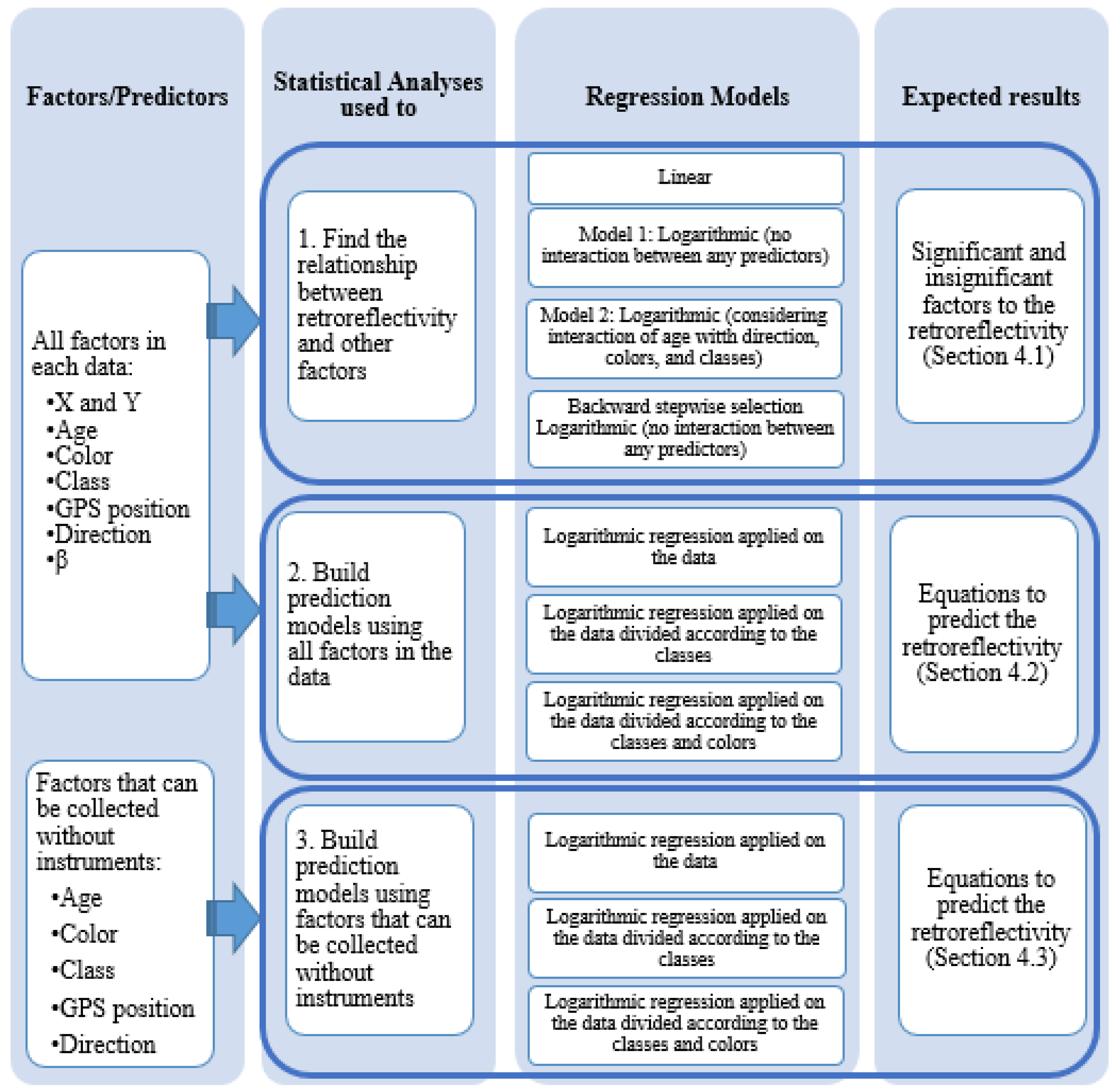
- Firstly, the relationship between retroreflectivity and other factors such as the CIE color coordinates, sign age, its class, GPS position, and direction are investigated. Linear and logarithmic regression models were conducted to identify the significant factors that affect retroreflectivity.
- Secondly, the study tries to find a connection between the performance and deterioration of retroreflectivity and the other factors mentioned above.
- Finally, the study proposes a way to analyze and calculate the performance and deterioration of retroreflectivity using factors that can be collected without using expensive instruments. Such factors include the traffic sign’s color, age, class, GPS position, and direction.
2. Systematic Literature Review
3. Materials and Methods
3.1. Data Description and Data Pre-Processing
- Class 1:
- Class 2:
- Class 3:
3.2. Statistical Analysis
4. Results and Discussion
4.1. The Relationship between Retroreflectivity and Other Factors
4.2. Prediction Models Using All Factors in the Data
4.3. Prediction Models Using Factors That Can Be Collected without Instruments
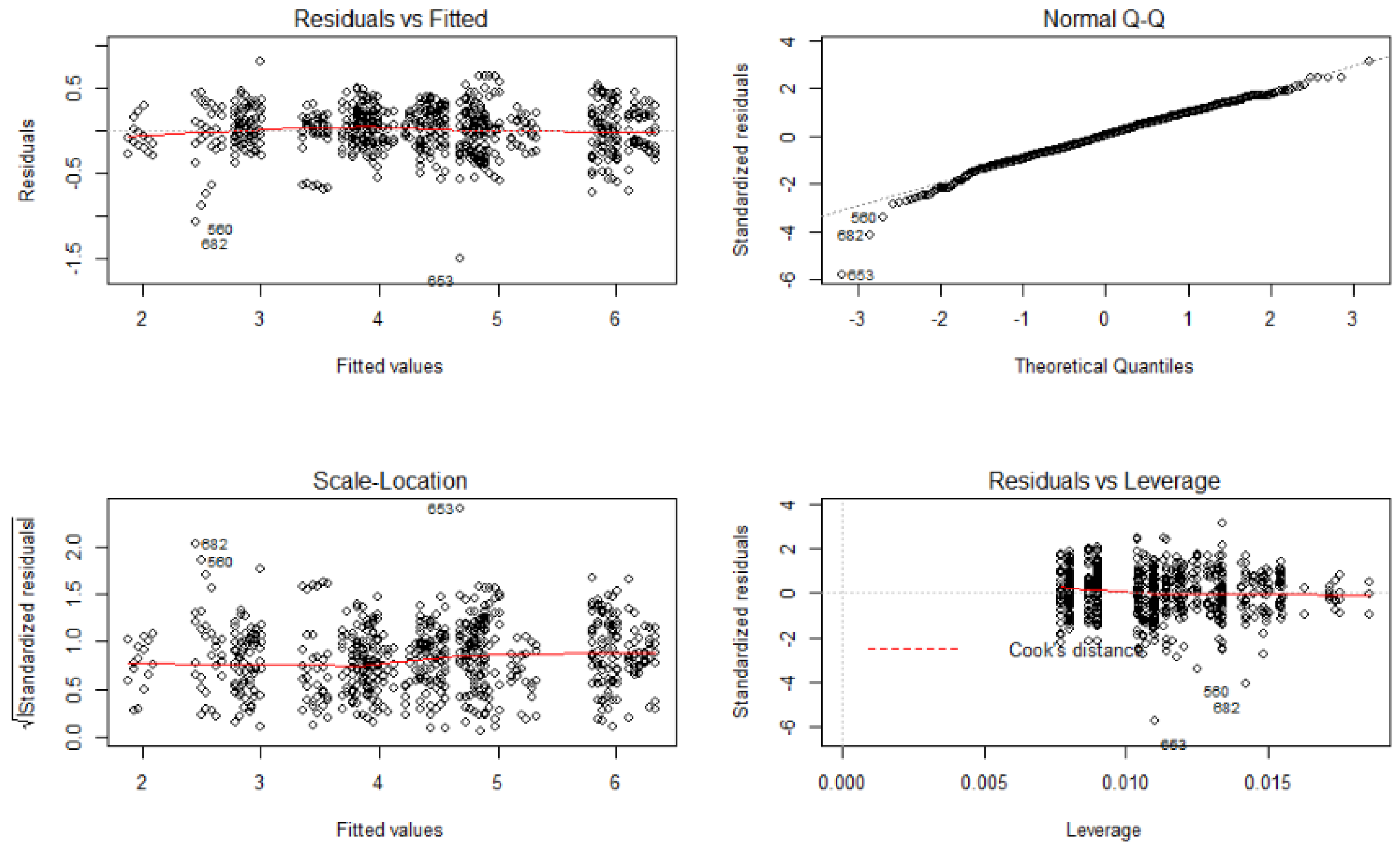
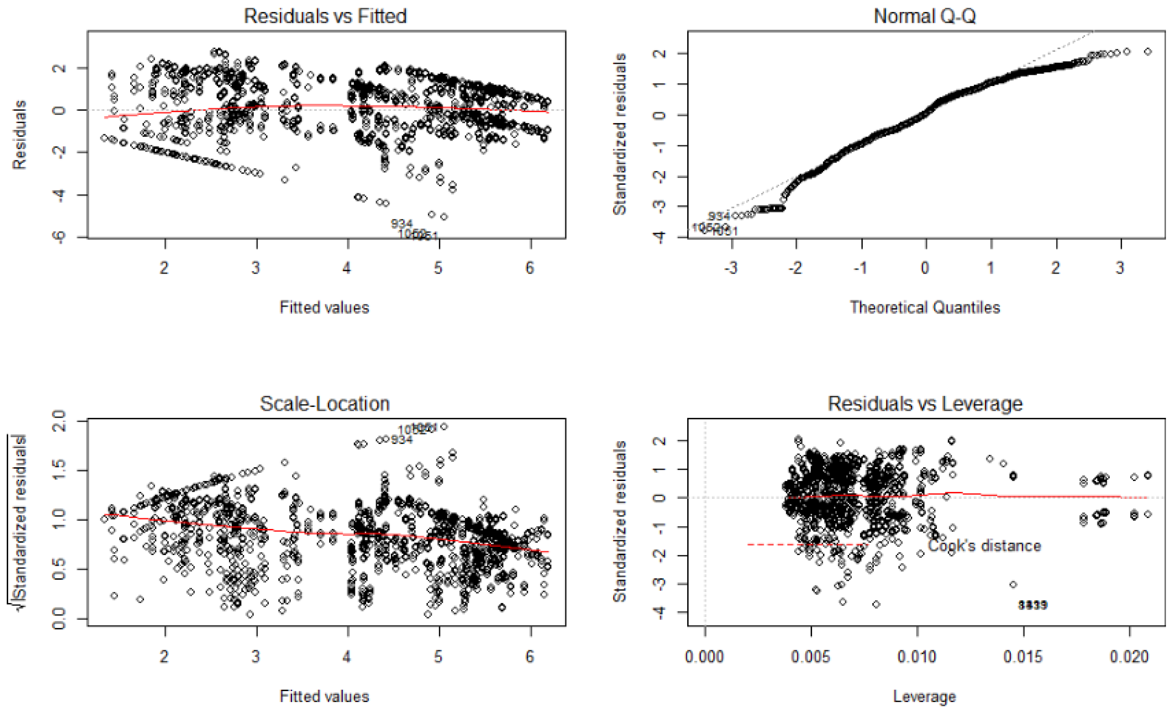
- The Residuals vs. Fitted values plot shows an almost horizontal line around the zero value. This indicates a linearity relationship between retroreflectivity and the predictors for the VTI and NMF data.
- The residuals are more normally distributed in the NMF data because the Normal Q-Q plot shows that the residual points almost follow the straight dashed line. However, the VTI data residuals follow the dashed line only in the middle part of the plot.
- The Scale-Location plot that was used to check the homogeneity of variance of the residuals (homoscedasticity) gives no indications of heteroscedasticity problems. A horizontal line with equally spread points is expected to indicate good homoscedasticity, and this is the case with both the VTI and NMF data.
- The Residuals vs. Leverage plots indicate the presence of some outliers in both datasets.
5. Limitations and Suggestions for Further Research
6. Conclusions
Author Contributions
Funding
Institutional Review Board Statement
Informed Consent Statement
Data Availability Statement
Conflicts of Interest
References
- Babić, D.; Babić, D.; Macura, D. Model for Predicting Traffic Signs Functional Service Life—The Republic of Croatia Case Study. Promet-Traffic Transp. 2017, 29, 343–349. [Google Scholar] [CrossRef] [Green Version]
- Costa, M.; Simone, A.; Vignali, V.; Lantieri, C.; Bucchi, A.; Dondi, G. Looking behavior for vertical road signs. Transp. Res. Part F Traffic Psychol. Behav. 2014, 23, 147–155. [Google Scholar] [CrossRef]
- Berzinsh, J.; Ozolinsh, M.; Cikmacs, P.; Pesudovs, K. Recognition of Retroreflective Road Signs during Night Driving. Human Factors in Transportation, Communication, Health, and the Workplace; Shaker Publishing: Maastricht, The Netherlands, 2002. [Google Scholar]
- Bible, R.C.; Johnson, N. Retroreflective Material Specifications and On-Road Sign Performance. Transp. Res. Rec. 2002, 1801, 61–72. [Google Scholar] [CrossRef]
- Hildebrand, E.D. Reductions in Traffic Sign Retroreflectivity Caused by Frost and Dew. Transp. Res. Rec. 2003, 1844, 79–84. [Google Scholar] [CrossRef]
- Swargam, N. Development of a Neural Network Approach for the Assessment of the Performance of Traffic Sign Retroreflectivity. Master’s Thesis, Louisiana State University, Baton Rouge, LA, USA, 2004. [Google Scholar]
- European Committee for Standardization. EN 12899-1. Fixed, Vertical Road Traffic Signs—Part 1: Fixed Sign. European Committee for Standardization: Brussels, Belgium, 2007; 57p. [Google Scholar]
- Ma, X.F.; Su, W.Y.; Li, D.; Wang, W. The Research for the Aging Performance of Reflective Sheeting by Artificial Accelerated Method. AMM 2013, 361–363, 2326–2329. [Google Scholar] [CrossRef]
- Alkhulaifi, A.; Jamal, A.; Ahmad, I. Predicting Traffic Sign Retro-Reflectivity Degradation Using Deep Neural Networks. Appl. Sci. 2021, 11, 11595. [Google Scholar] [CrossRef]
- Brimley, B.K.; Carlson, P. The Current State of Research on the Long-Term Deterioration of Traffic Signs. In Proceedings of the Transportation Research Board 92nd Annual Meeting and Publication in the Transportation Research Record, Washington, DC, USA, 13–17 January 2013. Paper 13-0033. [Google Scholar]
- Saleh, R.; Fleyeh, H. Factors Affecting Night-Time Visibility of Retroreflective Road Traffic Signs: A Review. Int. J. Traffic Transp. Eng. (IJTTE) 2021, 11, 115–128. [Google Scholar]
- Ré, J.M.; Miles, J.D.; Carlson, P.J. Analysis of In-Service Traffic Sign Retroreflectivity and Deterioration Rates in Texas. Transp. Res. Rec. 2011, 2258, 88–94. [Google Scholar] [CrossRef]
- Wolshon, B.; Degeyter, R.; Swargam, J. Analysis and Predictive Modeling of Road Sign Retroreflectivity Performance. In Proceedings of the 16th Biennial Symposium on Visibility and Simulation, Iowa City, IA, USA, 2–4 June 2002. [Google Scholar]
- Venkata, P.I.; Hummer, J.E.; Rasdorf, W.J.; Elizabeth, A.H.; Chunho, Y. Synthesis of Sign Deterioration Rates Across the United States. J. Transp. Eng. 2009, 135, 3. [Google Scholar]
- Huynh, N.; Mullen, R.; Pulver, Z.; Shiri, S. Sign Life Expectancy; Transport Research International Documentation (TRID): Washington, DC, USA, 2018. [Google Scholar]
- Immaneni, V.P.; Hummer, J.E.; Rasdorf, W.J.; Harris, E.A.; Yeom, C. Synthesis of sign deterioration rates across the United States. J. Transp. Eng. 2009, 135, 94–103. [Google Scholar] [CrossRef]
- Rasdorf, W.J.; Hummer, J.E.; Harris, E.A.; Immaneni, V.P.K.; Yeom, C. Designing an Efficient Nighttime Sign Inspection Procedure to Ensure Motorist Safety; North Carolina Department of Transportation: Raleigh, NC, USA, 2006. [Google Scholar]
- Venables, W.N.; Ripley, B.D. Modern Applied Statistics with S; Springer: New York, NY, USA, 2002. [Google Scholar]
- Osborne, J.W.; Waters, E. Multiple Regression Assumptions. ERIC Digest; ERIC Publications: College Park, MD, USA, 2002; ED470205. [Google Scholar]
- Osborne, J.W.; Waters, E. Four assumptions of multiple regression that researchers should always test. Pract. Assess. Res. Eval. 2002, 8, 2. [Google Scholar]
- Pawitan, Y. All Likelihood: Statistical Modeling and Inference Using Likelihood; Oxford University Press: Oxford, UK, 2001. [Google Scholar]
- Shao, C. Backward Selection—A Way to Final Model; PharmaSUG; Boehringer Ingelheim (China) Investment Co., Ltd.: Shanghai, China, 2019; Paper PO-077. [Google Scholar]


| References | Sheeting Types | Sheeting Colors | Models | Significant Factors | Insignificant Factors |
|---|---|---|---|---|---|
| Wolshon et al. [13] | I, III | green, white, yellow | Mathematical linear | Age | Orientation concerning the Sun, The distance from the road |
| Swargam [6] | I, III | green, white, yellow | Multi-linear regression, Artificial neural networks (ANNs) | Age | Orientation concerning the Sun, The distance from the road |
| Ré et al. [12] | III | red, white, yellow | Linear regression | Age, Region | Visual condition (daytime appearance, message integrity, and general condition), Orientation concerning the Sun |
| Babić et al. [1] | I, II, III | white, red, blue, yellow | Regression: linear, logarithmic, exponential | Age | |
| Alkhulaifi et al. [9] | I, II, III | green, white, blue, yellow | Deep neural network, Regression: linear, polynomial | Color, Observation angle, Sheeting type, Age | Sign orientation, Sheeting brand |
| VTI Data | NMF Data | |
|---|---|---|
| Variables | RA, X, Y, Age, Color, Class, Direction, GPSlat, GPSlong | RA, X, Y, β, Age, Color, Class |
| Number of studied samples/signs | 302 signs | 120 reflective sheeting samples |
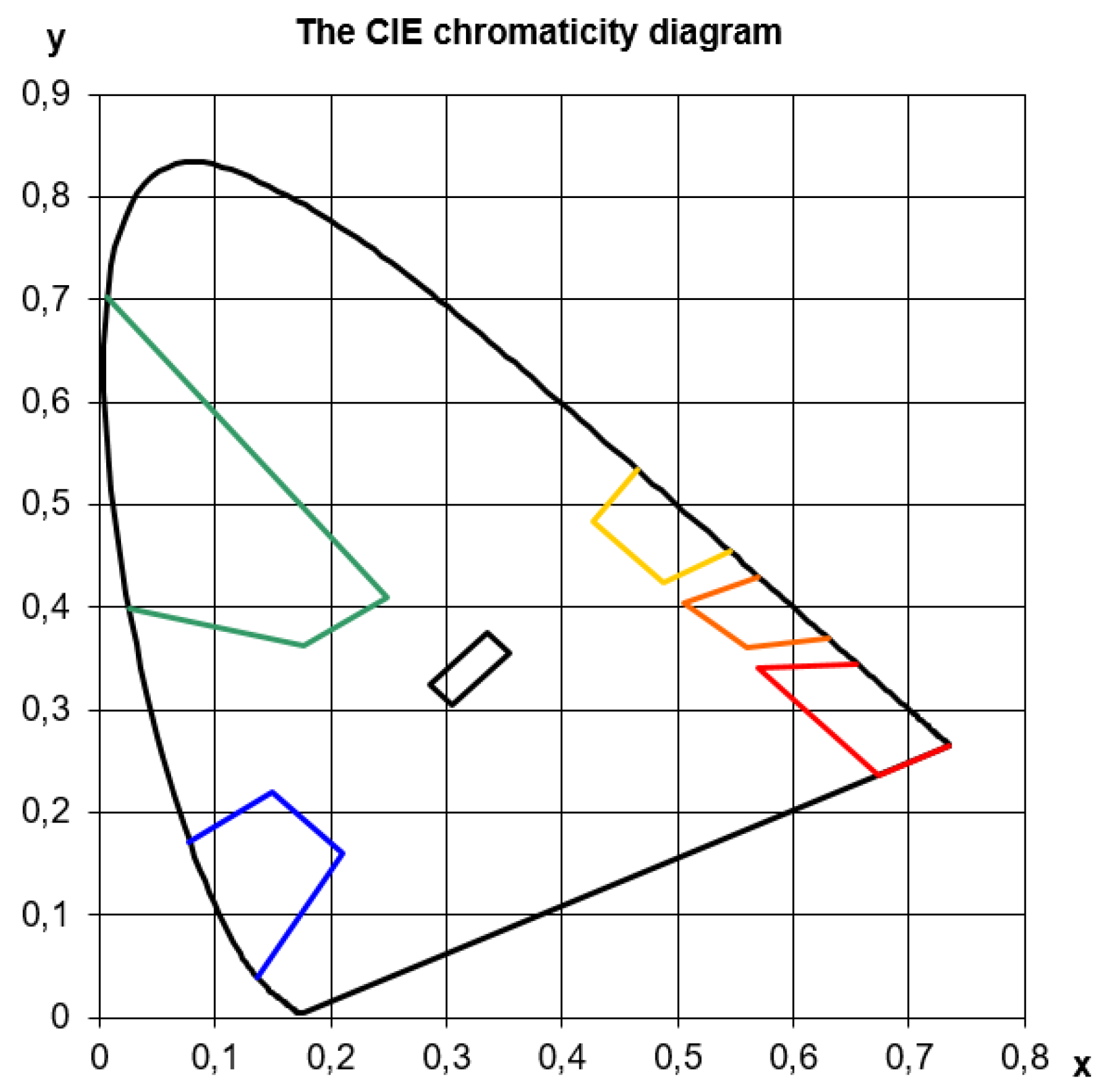
| Daylight chromaticity (X, Y) | Background and border | For each sample |
| Retroreflection values (RA) | Background and border | For each sample |
| Data collection | Data collected from different signs in 2018 | Data collected from the same samples once a year from 2015 to 2020 |
| Year of manufacture | (1983–2018) | 2015 |
| Direction | Azimuth direction (0–359 degrees) | Facing south and tilts 45° |
| GPS coordinates | Where the sign is mounted | Danish Technical University in Risø. |
| Type of retroreflection | Class 1, 2, and 3 | Class 1, 2, and 3 |
| Data size | 9 columns and 1813 rows | 7 columns * 717 rows |
| Factors | Linear Regression | Logarithmic Regression Model 1 | Logarithmic Regression Model 2 | Backward Selection 3 | ||||
|---|---|---|---|---|---|---|---|---|
| X | −615.12 | *** | −1.73 | *** | −1.85 | *** | −1.74 | *** |
| Y | 1086.71 | *** | 8.84 | *** | 8.85 | *** | 8.84 | *** |
| Green color | −88.19 | *** | −0.72 | *** | −0.53 | −0.71 | *** | |
| Red color | −18.65 | −0.46 | ** | −0.41 | −0.46 | ** | ||
| White color | 86.66 | *** | 0.05 | 0.58 | ** | 0.05 | ||
| Yellow color | −32.12 | * | −0.97 | *** | −1.11 | *** | −0.98 | *** |
| (Direction/360) | −10.05 | −0.25 | * | 0.10 | −0.25 | * | ||
| GPS latitude | 8.44 | ** | 0.12 | *** | 0.11 | *** | 0.12 | *** |
| GPS longitude | −2.54 | 0.01 | 0.03 | - | ||||
| Age | −3.34 | *** | −0.05 | *** | −0.07 | *** | −0.05 | *** |
| Class 2 | 42.77 | ** | 1.39 | *** | −0.24 | 1.39 | *** | |
| Class 3 | 254.47 | *** | 1.90 | *** | 1.16 | *** | 1.90 | *** |
| I (Direction/360): Age | −0.02 | * | ||||||
| Green color: Age | −0.02 | |||||||
| Red color: Age | −0.00 | |||||||
| White color: Age | −0.04 | *** | ||||||
| Yellow color: Age | 0.01 | |||||||
| Class 2: Age | 0.09 | *** | ||||||
| Class 3: Age | 0.06 | *** | ||||||
| R2 | 0.53 | 0.57 | 0.58 | 0.57 | ||||
| Factors | Linear Regression | Logarithmic Regression Model 1 | Logarithmic Regression Model 2 | Backward Selection 3 | ||||
|---|---|---|---|---|---|---|---|---|
| X | 34.19 | 1.45 | * | 1.68 | ** | 1.47 | ** | |
| Y | −231.24 | −0.58 | −0.72 | − | ||||
| β | −559.15 | *** | −0.30 | −0.30 | - | |||
| Green color | 106.85 | * | 0.75 | *** | 0.82 | *** | 0.57 | *** |
| Red color | 81.51 | 0.32 | 0.15 | 0.18 | ||||
| White color | 548.87 | *** | 2.34 | *** | 2.27 | *** | 2.09 | *** |
| Yellow color | 417.25 | *** | 1.79 | *** | 1.69 | *** | 1.51 | *** |
| Age | −4.36 | * | −0.04 | *** | −0.04 | ** | −0.04 | *** |
| Class 2 | 36.00 | *** | 0.88 | *** | 0.91 | *** | 0.89 | *** |
| Class 3 | 165.05 | *** | 1.88 | *** | 1.89 | *** | 1.89 | *** |
| Green color: Age | −0.01 | |||||||
| Red color: Age | 0.02 | |||||||
| White color: Age | 0.01 | |||||||
| Yellow color: Age | 0.02 | |||||||
| Class2: Age | −0.01 | |||||||
| Class3: Age | −0.00 | |||||||
| R2 | 0.74 | 0.95 | 0.95 | 0.95 | ||||
| DATA | Predictors | Class of Retroreflection | R2 |
|---|---|---|---|
| VTI | X + Y + Direction + GPSlat + GPSlong + Age + Color | 1 | 0.44 |
| 2 | 0.49 | ||
| 3 | 0.22 | ||
| NMF | X + Y+ β +Age + Color | 1 | 0.94 |
| 2 | 0.93 | ||
| 3 | 0.92 |
| Color | Class | VTI Data | NMF Data |
|---|---|---|---|
| Predictors: X + Y + Direction + GPSlat + GPSlong + Age | Predictors: X + Y + β + Age | ||
| Blue | 1 | 0.64 | 0.32 |
| 2 | 0.97 | 0.36 | |
| 3 | 0.73 | 0.21 | |
| Green | 1 | No green in Class 1 | 0.34 |
| 2 | No green in Class 1 | 0.49 | |
| 3 | 0.71 | 0.23 | |
| Yellow | 1 | 0.74 | 0.62 |
| 2 | 0.99 | 0.44 | |
| 3 | 0.81 | 0.07 | |
| Red | 1 | No red in Class 1 | 0.39 |
| 2 | 0.42 | 0.50 | |
| 3 | 0.97 | 0.63 | |
| White | 1 | 0.50 | 0.62 |
| 2 | 0.98 | 0.12 | |
| 3 | 0.74 | 0.50 |
| VTI Data | NMF Data | |||
|---|---|---|---|---|
| Predictors: Age + Direction + GPS Position + Color + Class | Predictors: Age + Color + Class | |||
| Linear Regression | Logarithmic Regression | Linear Regression | Logarithmic Regression | |
| R2 | 0.44 | 0.50 | 0.72 | 0.95 |
| Class | VTI Data | NMF Data | ||
|---|---|---|---|---|
| Predictors: Age + Direction + GPS Position + Color | Predictors: Age + Color | |||
| Linear Regression | Logarithmic Regression | Linear Regression | Logarithmic Regression | |
| 1 | 0.38 | 0.30 | 0.93 | 0.94 |
| 2 | 0.01 | 0.02 | 0.83 | 0.92 |
| 3 | 0.06 | 0.13 | 0.85 | 0.91 |
| Color | Class | VTI Data | NMF Data | ||
|---|---|---|---|---|---|
| Predictors: Age + Direction + GPS Position | Predictors: Age | ||||
| Linear Regression | Logarithmic Regression | Linear Regression | Logarithmic Regression | ||
| Blue | 1 | 0.31 | 0.25 | 0.10 | 0.12 |
| 2 | 0.02 | 0.01 | 0.22 | 0.29 | |
| 3 | 0.02 | 0.02 | 0.10 | 0.10 | |
| Green | 1 | - | - | 0.09 | 0.12 |
| 2 | - | - | 0.13 | 0.09 | |
| 3 | 0.04 | 0.04 | 0.09 | 0.10 | |
| Yellow | 1 | 0.57 | 0.58 | 0.07 | 0.06 |
| 2 | 0.00 | 0.01 | 0.05 | 0.06 | |
| 3 | 0.03 | 0.04 | 0.04 | 0.06 | |
| Red | 1 | - | - | 0.08 | 0.07 |
| 2 | 0.01 | 0.06 | 0.11 | 0.11 | |
| 3 | 0.04 | 0.03 | 0.08 | 0.09 | |
| White | 1 | 0.38 | 0.24 | 0.03 | 0.03 |
| 2 | 0.19 | 0.13 | 0.06 | 0.05 | |
| 3 | 0.06 | 0.05 | 0.03 | 0.04 | |
| Colors Included in the Model | Classes Included in the Models | VTI Data | NMF Data |
|---|---|---|---|
| Number of Observations | Number of Observations | ||
| All(blue + green + yellow + red + white) | All (1 + 2 + 3) | 1544 | 710 |
| 1 | 603 | 154 | |
| 2 | 258 | 191 | |
| 3 | 683 | 365 | |
| Blue | 1 | 196 | 32 |
| 2 | 98 | 42 | |
| 3 | 117 | 78 | |
| Green | 1 | - | 32 |
| 2 | - | 42 | |
| 3 | 60 | 78 | |
| Yellow | 1 | 205 | 32 |
| 2 | 24 | 42 | |
| 3 | 186 | 47 | |
| Red | 1 | - | 26 |
| 2 | 120 | 24 | |
| 3 | 192 | 47 | |
| White | 1 | 202 | 32 |
| 2 | 16 | 41 | |
| 3 | 128 | 84 |
Publisher’s Note: MDPI stays neutral with regard to jurisdictional claims in published maps and institutional affiliations. |
© 2022 by the authors. Licensee MDPI, Basel, Switzerland. This article is an open access article distributed under the terms and conditions of the Creative Commons Attribution (CC BY) license (https://creativecommons.org/licenses/by/4.0/).
Share and Cite
Saleh, R.; Fleyeh, H.; Alam, M. An Analysis of the Factors Influencing the Retroreflectivity Performance of In-Service Road Traffic Signs. Appl. Sci. 2022, 12, 2413. https://doi.org/10.3390/app12052413
Saleh R, Fleyeh H, Alam M. An Analysis of the Factors Influencing the Retroreflectivity Performance of In-Service Road Traffic Signs. Applied Sciences. 2022; 12(5):2413. https://doi.org/10.3390/app12052413
Chicago/Turabian StyleSaleh, Roxan, Hasan Fleyeh, and Moudud Alam. 2022. "An Analysis of the Factors Influencing the Retroreflectivity Performance of In-Service Road Traffic Signs" Applied Sciences 12, no. 5: 2413. https://doi.org/10.3390/app12052413
APA StyleSaleh, R., Fleyeh, H., & Alam, M. (2022). An Analysis of the Factors Influencing the Retroreflectivity Performance of In-Service Road Traffic Signs. Applied Sciences, 12(5), 2413. https://doi.org/10.3390/app12052413