Expandable Spherical Projection and Feature Concatenation Methods for Real-Time Road Object Detection Using Fisheye Image ^†

Abstract

Fisheye lens cameras are widely used in such applications where a large field of view (FOV) is necessary. A large FOV can provide an enhanced understanding of the surrounding environment and can be an effective solution for detecting the objects in automotive applications. However, this comes with the cost of strong radial distortions and irregular size of objects depending on the location in an image. Therefore, we propose a new fisheye image warping method called Expandable Spherical Projection to expand the center and boundary regions in which smaller objects are mostly located. The proposed method produces undistorted objects especially in the image boundary and a less unwanted background in the bounding boxes. Additionally, we propose three multi-scale feature concatenation methods and provide the analysis of the influence from the three concatenation methods in a real-time object detector. Multiple fisheye image datasets are employed to demonstrate the effectiveness of the proposed projection and feature concatenation methods. From the experimental results, we find that the proposed Expandable Spherical projection and the LCat feature concatenation yield the best AP performance, which is up to 4.7% improvement compared to the original fisheye image datasets and the baseline model.

1. Introduction

Comprehensive information about the environment is one of the important properties of advanced driver-assistance system (ADAS). In order to thoroughly understand the road scenes, it is necessary to detect all the relevant surrounding objects with a sufficient range of view. During the last few years, deep-learning based methods show the most promising performance with the development of open-source frameworks [1,2,3,4,5]. This approach requires a relatively large computational resource, but modern hardware can easily be adapted to real-time detection.

One of the core features in systems-on-board autonomous vehicles is perception. A combination of sensors, such as cameras, radar, lidar, and GPU, are used to collect the data around the environment and extract the relevant information in the perception stage. In a low-cost sensor setup, 2D cameras with a large field of view (FOV) can efficiently cover a large area around the vehicle and ensure the safety of the autonomous driving. Especially, the fisheye camera can obtain visual information with a more than 180° field of view, thus the fisheye camera is widely used in ground, aerial, and underwater autonomous robot as well as surveillance [6,7,8].

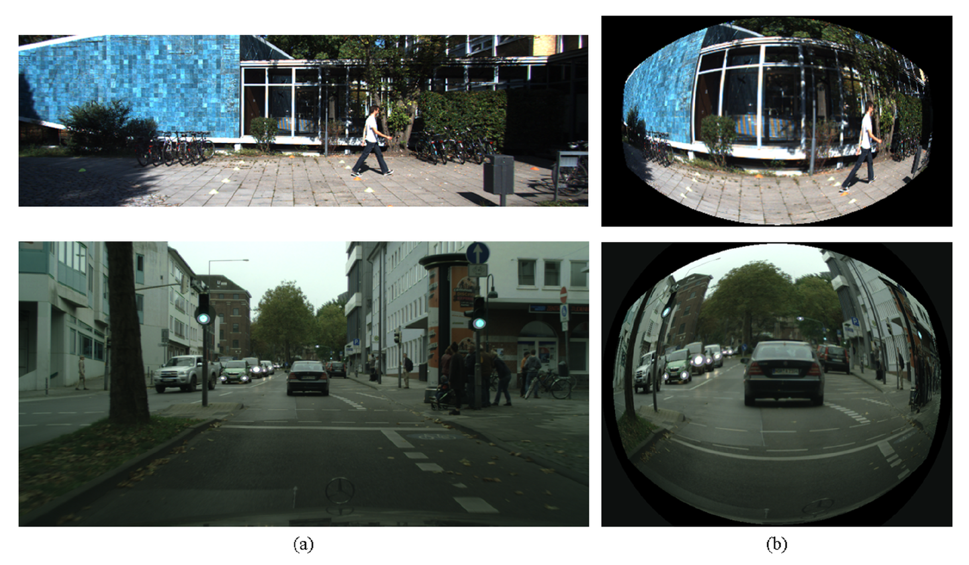
However, this advantage comes at the cost of strong radial distortion. The resulting issues, such as curving and diagonal tilting of objects are increasingly severe towards the edges of the fisheye image. Therefore, the shapes of the objects in the same category are less conformal to each other in different images and the target bounding box contains more unnecessary background. Another notable feature of the fisheye camera is that both relative size and distance are exaggerated. The ultra-wide angle lens shows nearby objects appear much larger, while objects located far away or in the boundary appear much smaller than the lens of perspective cameras. Consequently, the already poor performance of object detectors for small or tiny objects is further degraded.

Due to the unique feature of the strong radial distortion, object detection in the fisheye image must solve the two problems:

• Relatively different object size depending on the location and distance.
• Inherent Curving and diagonal tilting of objects in the boundary area.

To solve these problems, many investigations have been introduced and they are categorized in the following two main approaches:

• Object detection using the original fisheye image.
• Object detection after fisheye image rectification or undistortion.

The first approach is using the original image. Instead of fisheye image rectification or undistortion, they investigate distortion-invariant or rotation-invariant neural networks. SphereNet [9] suggests a distortion-invariant neural network for the omnidirectional images, adapting the sampling grid locations of a convolutional kernel. The SphereNet kernel uses the projection of the spherical camera model to the tangent plane on the sphere, yielding filter outputs which are invariant to latitudinal rotations.

Alternatively, a rotation-invariant model which predicts object orientations is proposed by [10,11]. In [10], the original fisheye image is used without undistortion to avoid the bottleneck in achieving real-time recognition performance. The road object such as vehicle and pedestrian are rotated in the boundary of the original fisheye image, thus the authors proposes a rotation invariant deep neural network. In contrast, a rotation sensitive neural network is proposed in [11] to detect objects in the original fisheye image. The bounding box is rotated to fit the orientation of the detecting object. However, these two investigations detect road or indoor objects which size is normal compared with the image size. In their test images, the sizes of the bounding boxes of pedestrian, vehicle, and computer monitor are generally large compared with the image size.

In [12], the original fisheye image is trained without any lens parameters or calibration patterns. Instead, the authors propose a contour-based object detector to cope with the distortion of the fisheye image. A ’distortion shape matching’ strategy is proposed to train the contour information of objects using a fisheye image detection network. A small object detection method in the fisheye image is proposed in [13]. The authors propose a concatenated feature pyramid, which is a variant of the Feature Pyramid Network (FPN), to find very small road objects in a fisheye image. They add an additional concatenation network to the original FPN in YOLOv3 to increase the small object detection performance.

The second approach is based on the rectification or undistortion of the original fisheye image. The generative-adversarial network is adapted to rectify the fisheye image in [14,15]. However, these studies require complex computations, hindering the real-time performance that are required from one-stage object detectors. The cylindrical projection model is also used to rectify the fisheye image and to find the 3D objects in the road scene [16]. The authors propose that training the rectilinear images is better than using the original fisheye image for detecting the 3D road objects. The authors use their own fisheye image database for performance comparison. The images are captured by using a side view camera, thus the number of road objects is smaller than that in the standard benchmark.

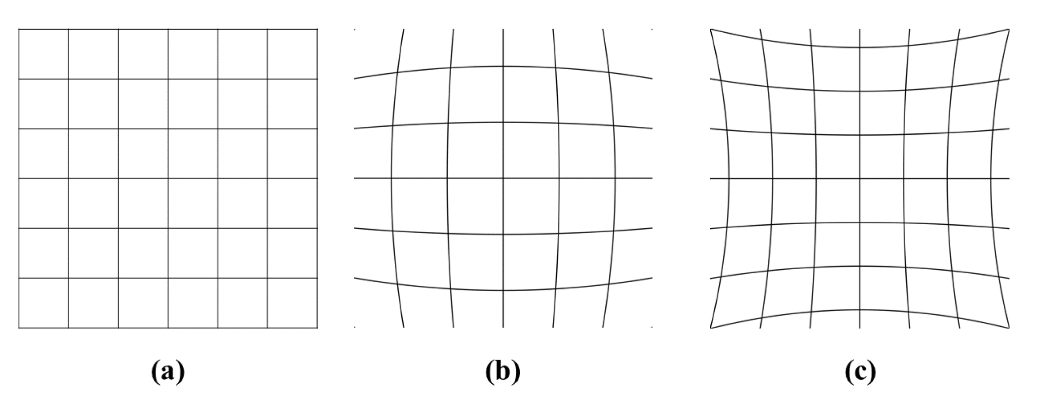
As described above, recent investigations on the fisheye image object detection mostly utilize the original image rather than using rectification or undistortion method. This is due to the strong radial distortion of the fisheye image. Some investigations utilize the conventional cylindrical or spherical rectification; however, the rectified images still contain object size variation due to barrel or pincushion distortions.

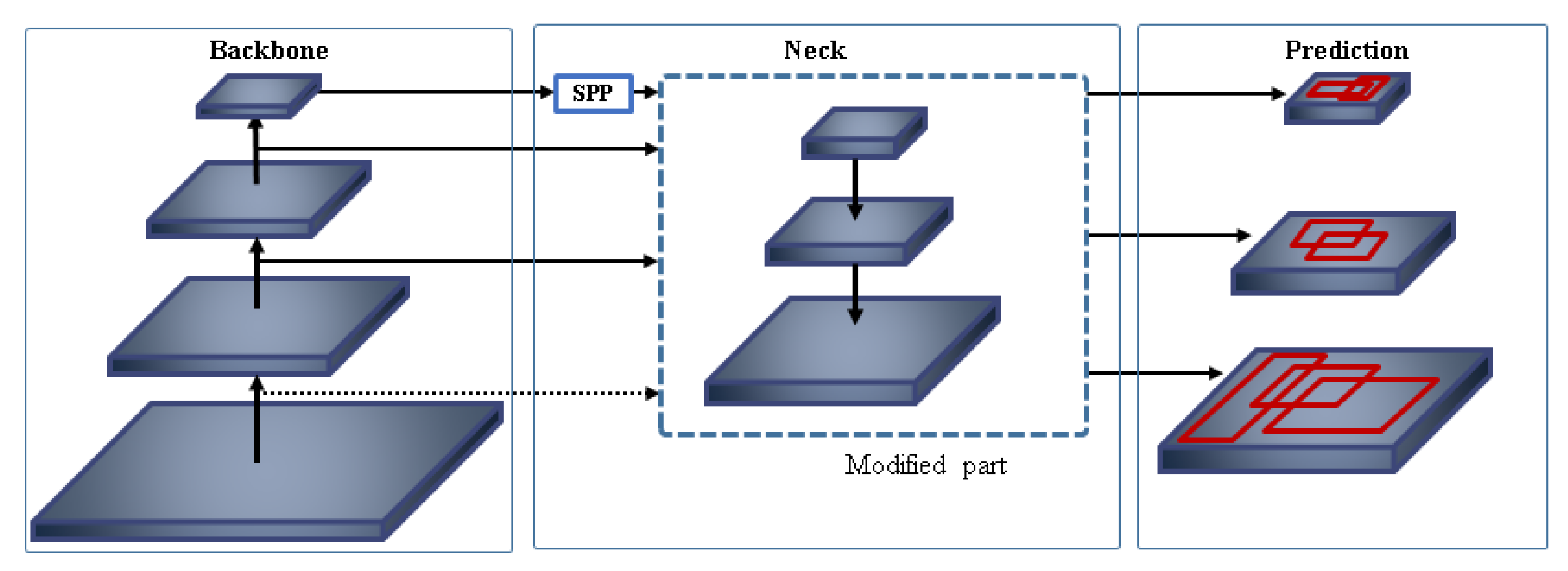
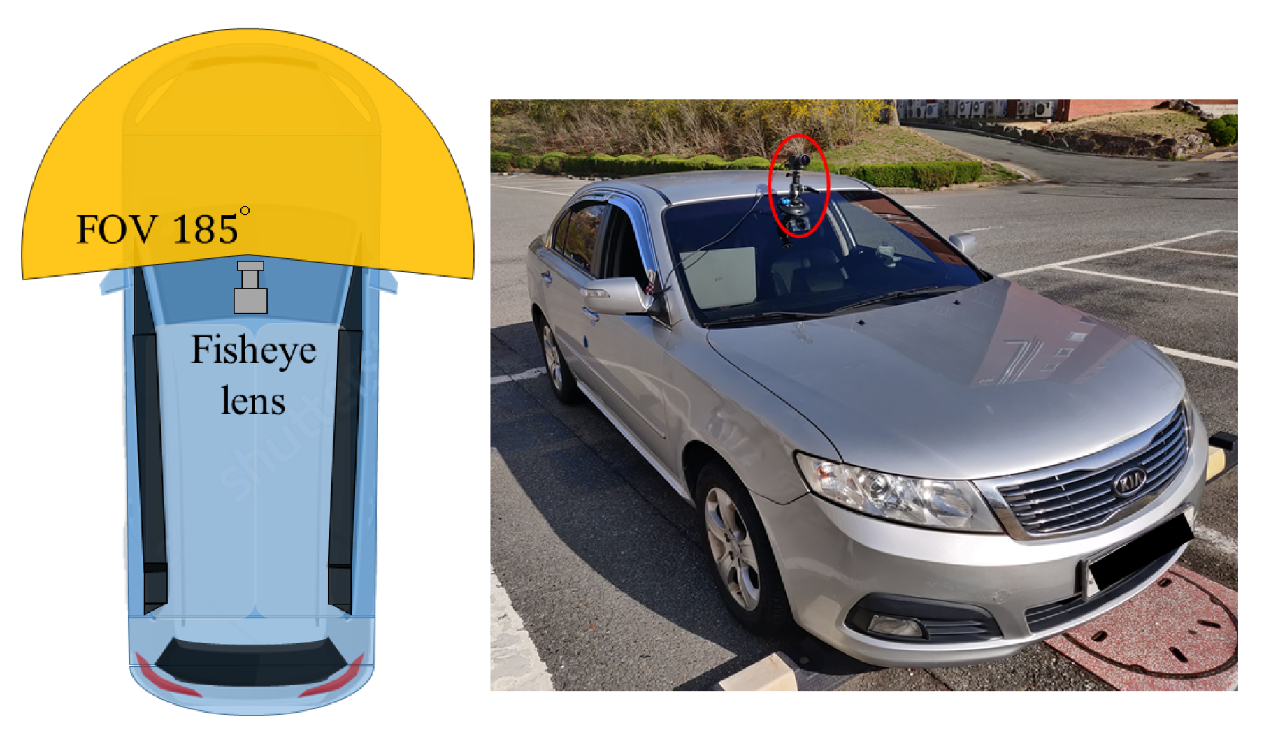
Therefore, in this paper, we first propose a new spherical-based projection in real-time speed to solve radial distortion and detect small objects with increased pixel information. Second, we propose a multi-level feature concatenation to a convolutional neural network, suggesting three types of concatenated YOLOv3 with Spatial Pyramid Pooling (SPP) module [17,18,19,20]. We evaluate our solution with several public datasets, as well as our new collection of images gathered with a 185° fisheye lens. The major contributions of this study are noted as follows.

• Introduction of a new front-view fisheye dataset consisting of 5K bounding box annotations.
• Proposal of an effective spherical projection model on fisheye images based on the size of objects in the dataset.
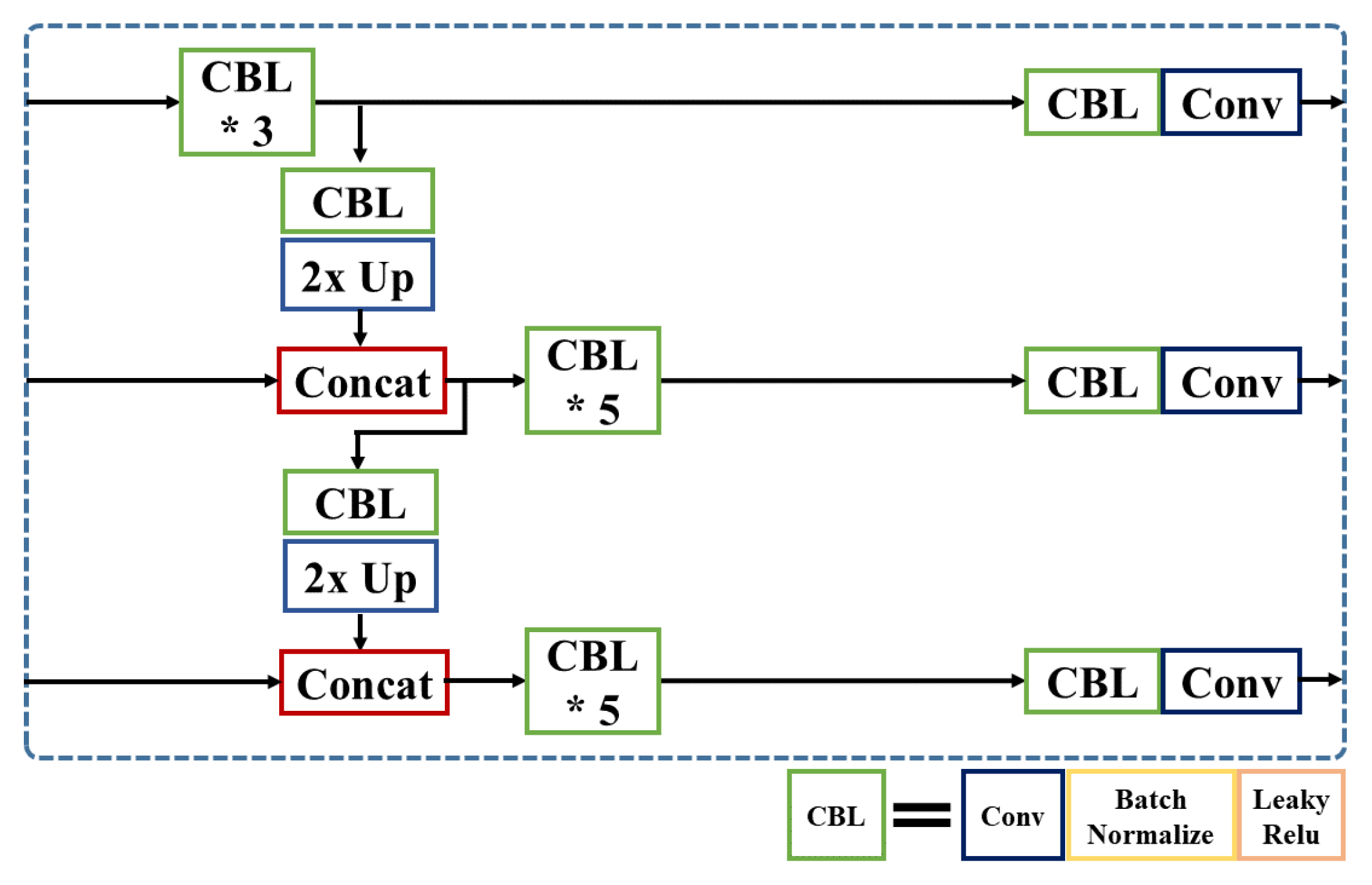
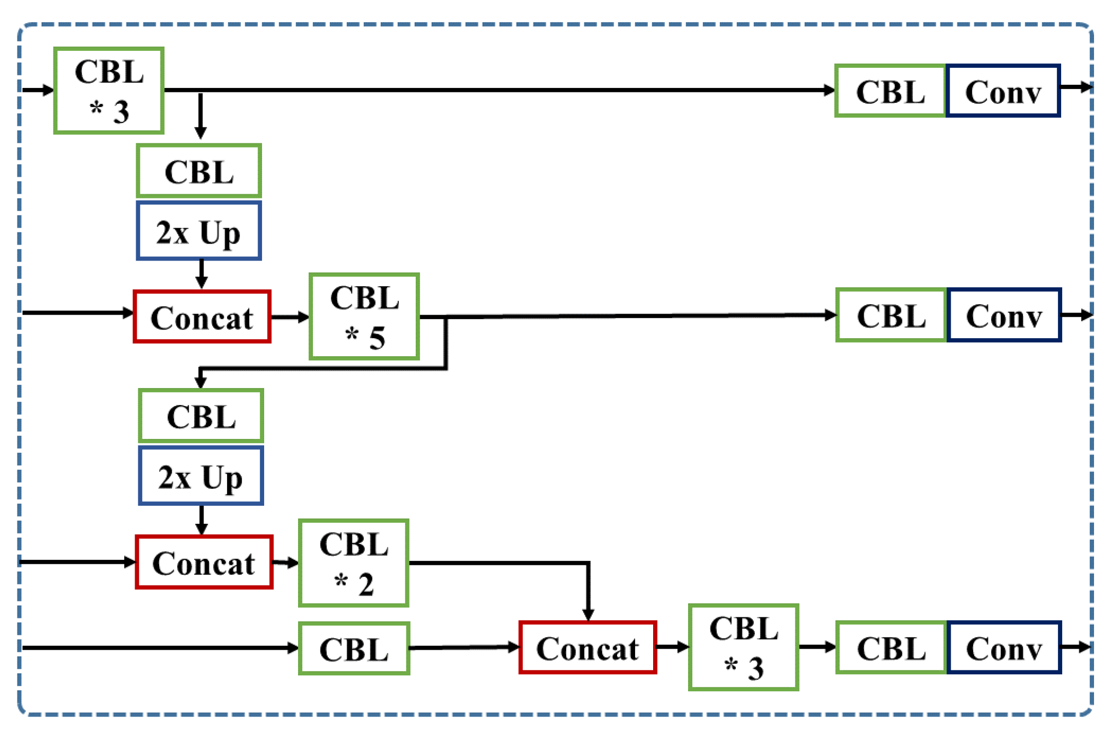
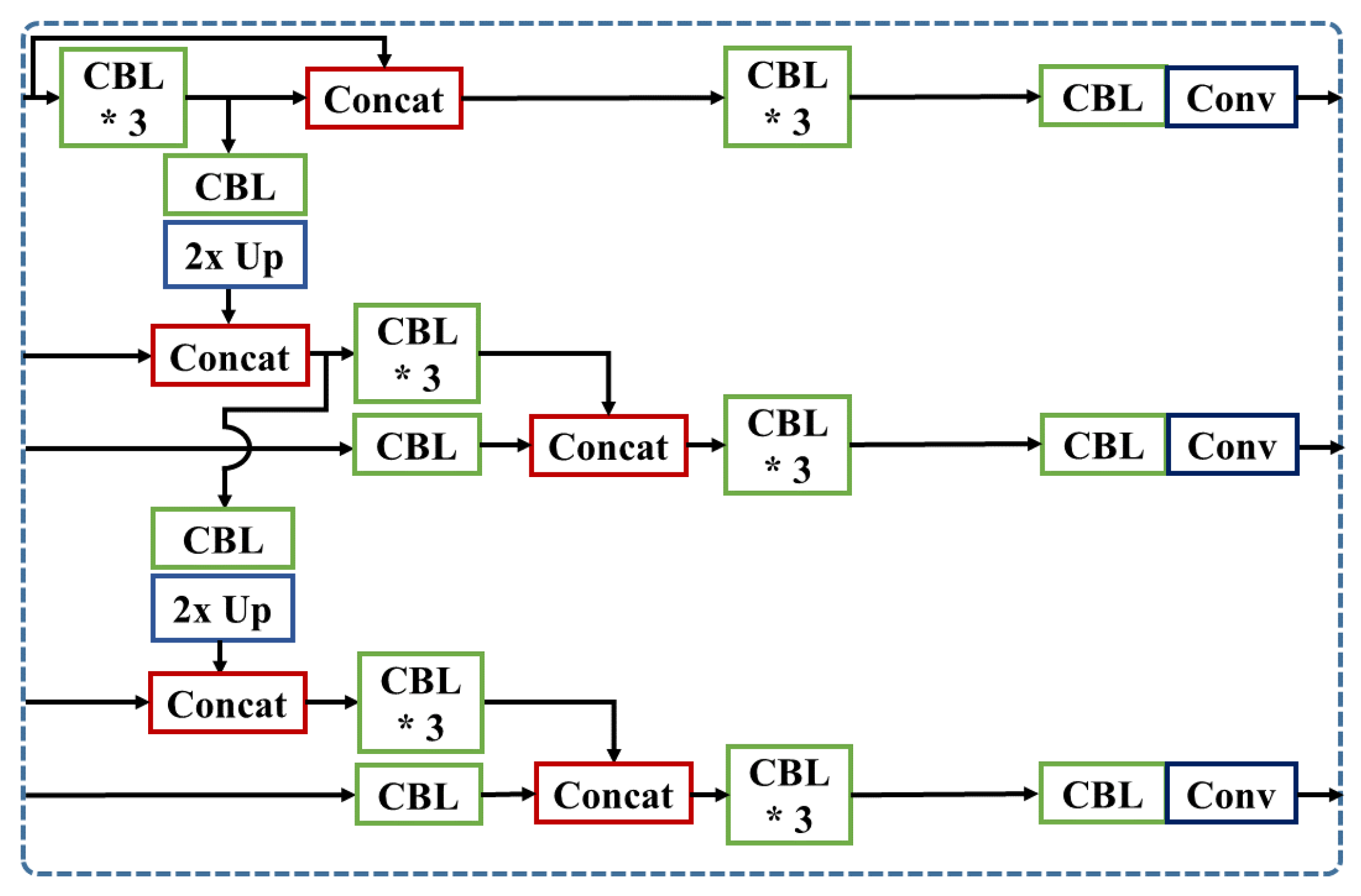
• Proposal and analysis of three feature concatenation methods to reduce small objects detection issues in real-time object detector.

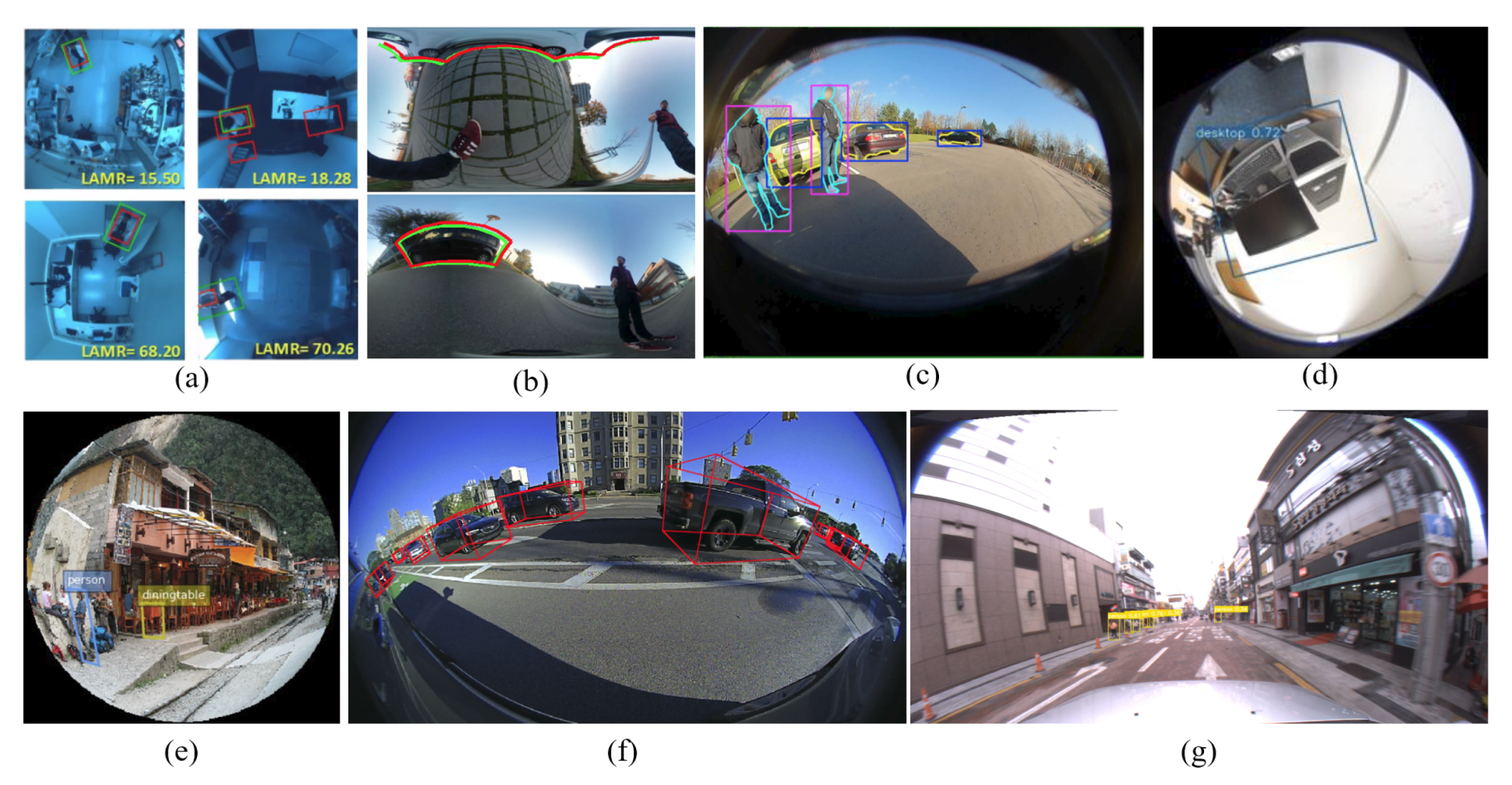
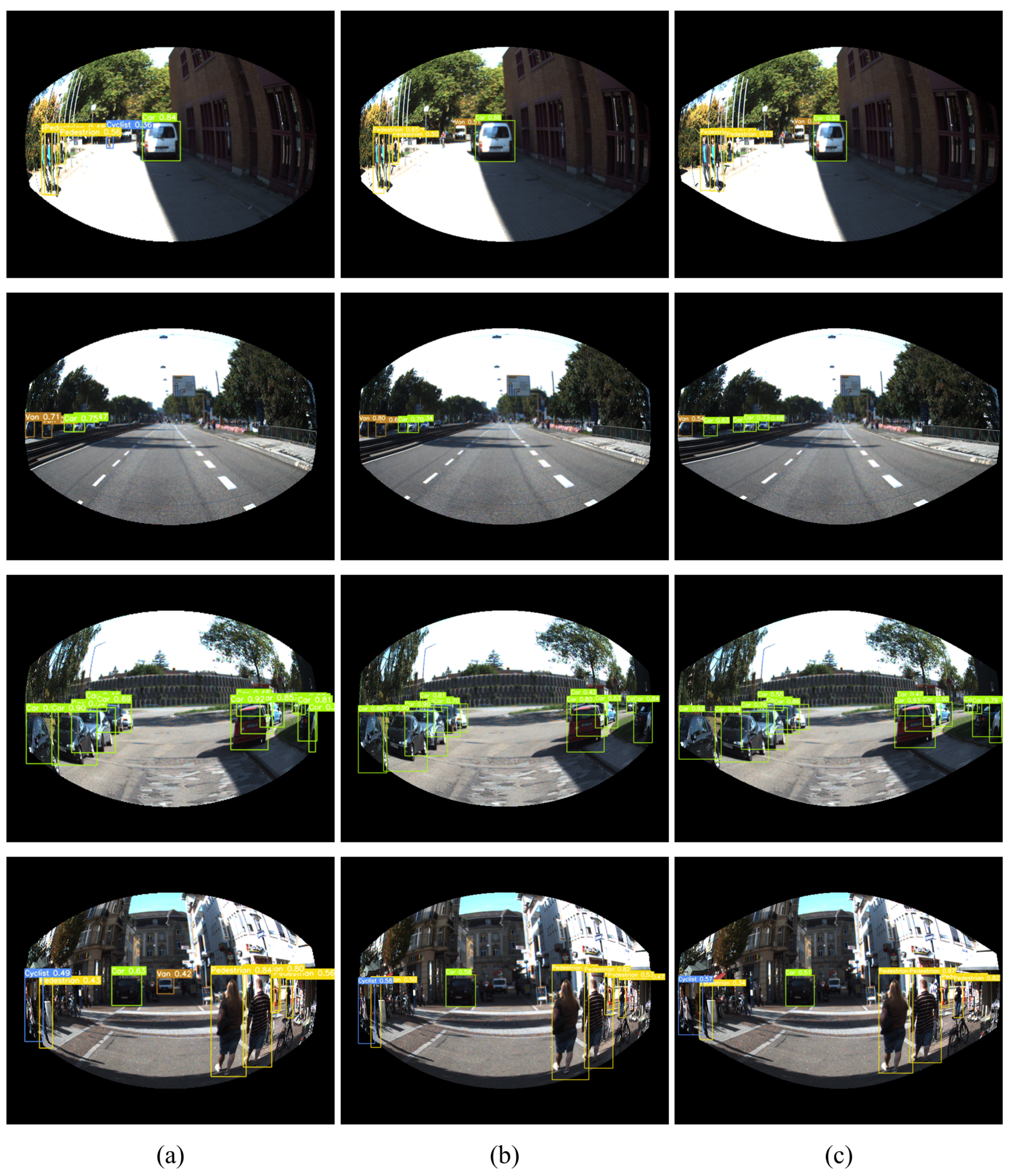
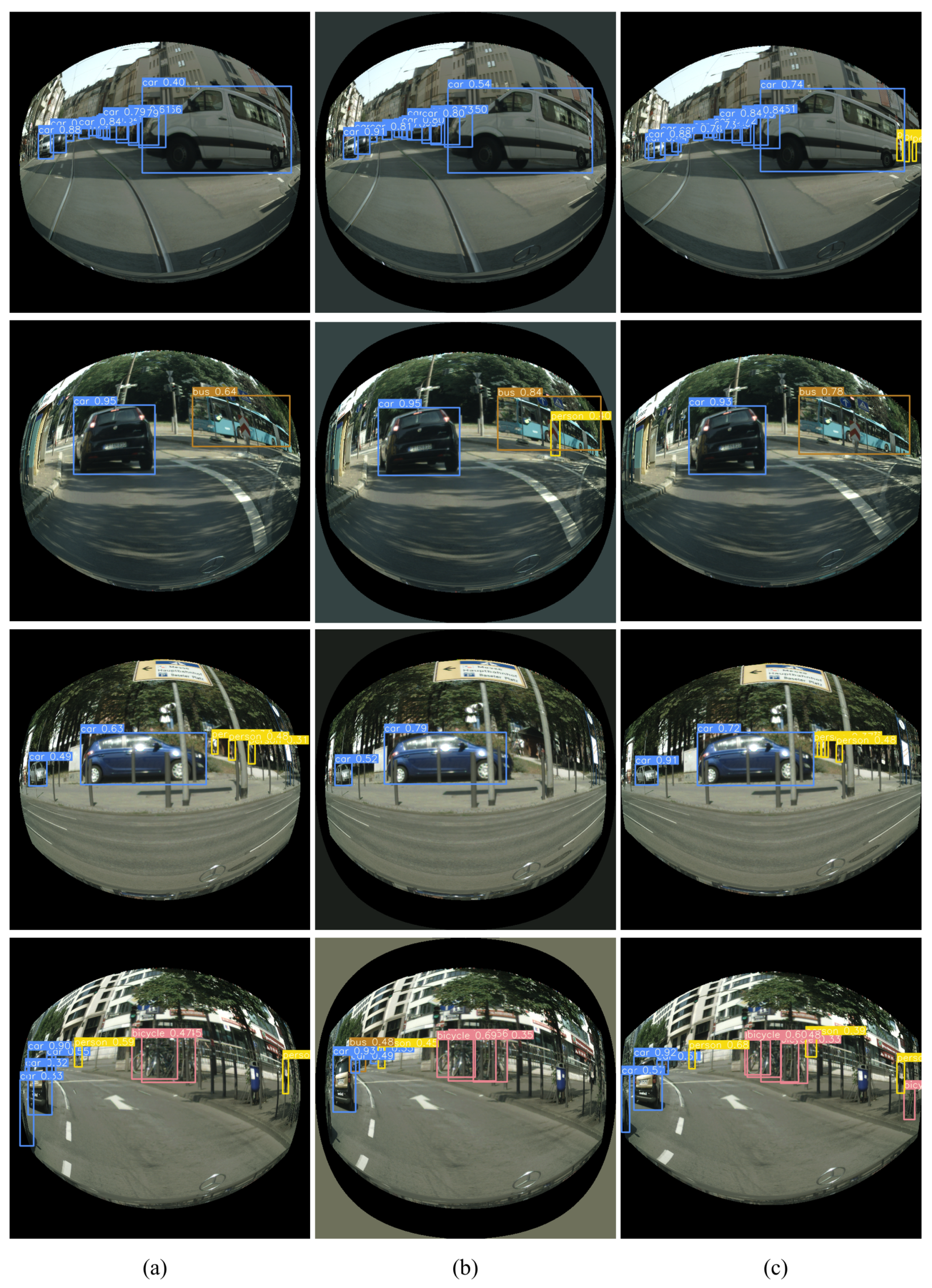
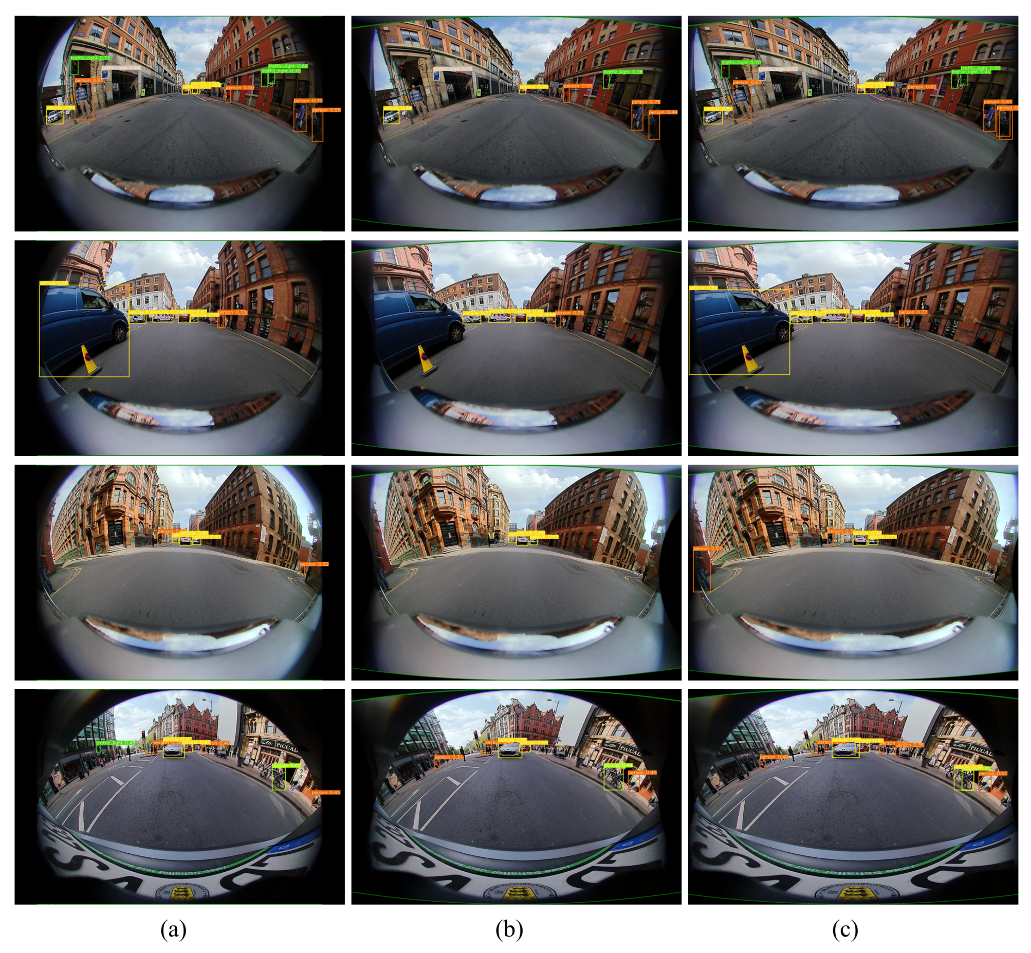
Figure 1 shows some examples of object detection bounding boxes from several types of fisheye images. The size of bounding boxes is different according to the size of the detected objects. In the previous investigations, the detected objects are generally large in the image. Thus, the detection is relatively easier than small or tiny objects. In contrast, in this paper, we propose a deep neural network to detect not only regular but also small or tiny road objects. In one of our results in Figure 1g, the bounding box size of the detected object is very tiny compared with the size of the rectified image. To achieve the best performance of tiny object detection, we propose a new spherical projection model and feature concatenation methods.

In Section 2, we describe related works on commonly used fisheye camera projection models, fisheye lens dataset, and deep-learning-based object detection models. Section 3 briefly describes the proposed projection algorithm, the details of the experimental setup, and concatenated model design. In Section 4, we present the experiments and analysis of the results. Finally, Section 5 and Section 6 discuss the quantitative improvement of the proposed method based on the results of four datasets and conclude the paper.

2. Related Works

2.1. Fisheye Camera Projection

Fisheye lens can cover large areas in a circular image with more than 100° horizontal field of view, but results in considerable distortions. Figure 2 illustrates the common types of the distortion from modern cameras. Barrel distortion, as shown in Figure 2b is the apparent effect of the fisheye image. Image magnification of this distortion reduces with the distance from the optical axis, presenting straight lines to be curved outwards which is a similar shape as the barrel. On the other hand, the pincushion distortion shown in Figure 2c shows more magnification with the distance from the optical axis, showing the lines curved towards the center of the image.

Consequently, several rendering methods have been studied to minimize these distortions. The most representative method is to reproject the fisheye image to the undistorted image by using the principle of fisheye camera models, such as spherical, cylindrical, and rectilinear projection [11,21]. The camera model describes how three-dimensional (3D) world points are projected into two-dimensional (2D) pixel coordinates. Fisheye image correction can be accomplished by the process of mapping the points in the spherical coordinates $\theta$ and $\varphi$ to the image coordinates x and y.

2.1.1. Rectilinear Projection

Rectilinear projection, also called as “perspective”, “gnomonic”, or “tangent-plane” projection, is mostly used for the calibration of general cameras. This projection maps a portion of the surface of a sphere to a flat image [22], proceeding as follows:

$$\begin{array}{cc}\hfill x=& \frac{cos\varphi sin(\theta -{\theta }_0)}{sin{\varphi }_{1}sin\varphi +cos{\varphi }_{1}cos\varphi cos(\theta -{\theta }_0)},\hfill \\ \hfill y=& \frac{cos{\varphi }_{1}sin\varphi -sin{\varphi }_{1}cos\varphi cos(\theta -{\theta }_0)}{sin{\varphi }_{1}sin\varphi +cos{\varphi }_{1}cos\varphi cos(\theta -{\theta }_0)}.\hfill \end{array}$$

(1)

The main advantage is that it renders the straight lines in 3D world to the straight lines in 2D images. However, the objects and structures are significantly stretched towards the corners and look more unnatural with a larger view. Therefore, this projection is recommended when a horizontal and vertical FOV is less than 120°.

2.1.2. Cylindrical Projection

Cylindrical projection maps the horizontal coordinate to the longitude $\theta$. For the vertical coordinate, it projects a surface of a sphere onto a cylinder using the tangent of latitude $\varphi$, which can be envisioned by surrounding the circumference of the sphere with a flat piece of paper. Using the cylindrical projection, several authors estimate the depth from wide angle cameras [21,23]. The projection is expressed as follows:

$$\begin{array}{cc}\hfill x& =\theta ,\hfill \\ \hfill y& =tan\varphi .\hfill \end{array}$$

(2)

Since it stretches the object vertically with the tangential operation, the vertical field of view has a physical limit of 180°. In addition, vertically-longer-image distorts objects narrower which can hinder the accurate detection when using square kernel type of standard convolutional neural network.

2.1.3. Spherical Projection

Spherical projection, also called as “equirectangular” or “equidistant cylindrical” projection, maps the longitude and latitude linearly to horizontal and vertical coordinates:

$$\begin{array}{cc}\hfill x& =\theta ,\hfill \\ \hfill y& =\varphi .\hfill \end{array}$$

(3)

Because of its simple relationship between the position of an image pixel and its corresponding 3D location, this projection is used in many applications for mapping a surface of a sphere to a flat image.

Some works have successfully demonstrated in 2D object detection in panoramic images with standard convolutions [24], and in omnidirectional images with non-standard convolutions [9]. The advantage of spherical projection is that it can support the vertical field of view of the fisheye lens over 180°. Additionally, it generates fewer vertically-long objects compared to cylindrical projections, since the spherical projection maps meridians and latitude to the lines with constant spacing. Therefore we use spherical-based projection to the fisheye images in this study.

2.2. Fisheye Dataset for Urban Driving

2.2.1. Synthetic Dataset

Generating a large volume of the dataset is a highly time-consuming task. To handle this issue, some works suggest leveraging open-source datasets with commonly used camera models.

In a similar way, two well-known datasets, VOC2012 [25] and Wider Face [26] are synthesized to fisheye images in [27]. For the stereo algorithm, 45k synthetic fisheye images in four orthogonal directions are presented in [28]. In our work, we use synthetic as well as real fisheye datasets. The synthetic fisheye images are generated from CityScape [29] and KITTI [30] dataset following the method in ERFNet [31]. Since the CityScape dataset is intended for a semantic segmentation task, we convert original annotations to bounding box format. The example images are shown in Figure 3.

2.2.2. Real Dataset

Several authors have considered the fisheye cameras for ego vehicles. Among them, some notable works are classification and tracking of cars and pedestrians using hybrid cameras [32], pedestrian detection using a combination of synthetic and real images from a 360° horizontal FOV camera [33]. In addition, WoodScape [34] is a multi-camera fisheye dataset, providing 360° sensing around a vehicle with four fisheye lenses.

At the beginning of our work, there was no publicly available fisheye dataset with object detection-related labels. Therefore, we collected our own fisheye images with one 185° FOV lens and labeled the bounding box for nine object classes. In addition, we employed the newly open-source dataset WoodScape which is comprised of nine tasks including 2D bounding box detection.

2.3. Object Detection Model

The latest object detection models are commonly sorted into two types: one-stage detector and two-stage detector. For applications, where faster inference is required, typically a one-stage detector which directly predicts bounding boxes (bbox) and classes is used. On the contrary, the two-stage model first extracts region proposals, before predicting the exact bboxes and the corresponding classes to those locations. Since we aim for real-time performance, a one-stage detector will be chosen.

As for the one-stage model, anchor-based and anchor-free detectors are frequently studied. The anchor box is a predefined bbox of a certain height and width. Among anchor-free detection methods, keypoint detection [5,35,36] utilizes a center, or a corner point, without using any predefined anchors. An alternative way is to detect the objects with pixel-wise prediction [37].

In anchor-based detectors, the bounding boxes are defined to capture the scale and aspect ratio of target object classes. During detection, the predefined anchor boxes are tiled across the image. The most popular anchor-based network are the various versions of YOLO [17,18,38].

YOLOv3 [17] makes the prediction at three different scales based on feature pyramid networks structure [39]. Additionally, it adopts up-sampling layers concatenated with the previous layers to preserve the detailed features. Moreover, this algorithm uses more anchor boxes, logistic regression for label prediction, multi-label classification, and deeper backbone model Darknet-53.

To develop a more efficient network, the YOLOv4 has been released by applying “Bag of freebies” and “Bag of specials”. Bag of freebies are the training strategies that only change the cost in the training procedure and Bag of specials includes plugin modules or post-processing methods that only increase the inference cost for higher improvement in the detection accuracy. Despite the advantages of YOLOv4, we employ YOLOv3 in this study because it was used to lay the groundwork that is extended here from prior work. Moreover, many functionalities of the “Bag of freebies” and “Bag of specials” of YOLOv4 can be implemented in this framework as well.

In this paper, we exploit the concatenation layer which can capture the spatial information from the shallower layer, and semantic features from the deeper layer which improves the detection performance of small objects [13,40]. Therefore, we suggest additional concatenation modules with three variants based on YOLOv3-SPP for extracting more meaningful information for small objects in fisheye images [41]. Figure 4 presents the structure of the baseline and each concatenated model.

3. Proposed Method

3.1. Training Data

3.1.1. Label Transformation

Among our datasets, the CityScape originally has fine pixel-level annotation files for dense semantic segmentation. To employ this data to our algorithm, we first selected necessary classes for object detection. Our custom categories are composed of 10 different objects: person, rider, car, truck, bus, train, motorcycle, bicycle, caravan, trailer. For the group classes consisting of multiple objects, such as person group, car group, and bicycle group, we manually separated and re-annotated by one object unit. Second, we extract four corner points of the objects $x_{min}$, $x_{max}$, $y_{min}$, $y_{max}$ from the polygon values consisting of pixel points ($x_i$, $y_i$) of object boundary which are expressed as follows:

$$\begin{array}{cc}\hfill x_{min}& =\underset{x_i}{min}(x_1,\dots ,x_n),\hfill \\ \hfill y_{min}& =\underset{y_i}{min}(y_1,\dots ,y_n),\hfill \\ \hfill x_{max}& =\underset{x_i}{max}(x_1,\dots ,x_n),\hfill \\ \hfill y_{max}& =\underset{y_i}{max}(y_1,\dots ,y_n).\hfill \end{array}$$

(4)

Since the label format of YOLO is based on the relative values, we convert the absolute corner points to a relative one center point with the size of the bounding box.

3.1.2. Dataset Collection

Circular fisheye images from the Fujinon FE185C057HA-1 lens with 1.8 mm focal length and 185° FOV were captured with a FLIR Grasshopper 3 GS3-U3-28S4C-C Camera. Since a front view is the most important vision of the autonomous driving, we installed the camera to the front window of the vehicle as illustrated in Figure 5.

The data, consisting of 21k road scenes in Daegu Dongseongro, South Korea, were gathered during cloudy and drizzling weather. Bounding boxes were manually annotated to 5k images.

3.2. Expandable Spherical Projection

The idea of spherical projection is to project the distorted fisheye image into the undistorted cylinder image, whose equal distances measured from the center correspond to equal steps in the angle of 3D scene. The mathematics of this projection can be expressed in longitude and latitude coordinate systems.

$$\begin{array}{cc}\hfill x_n& =\frac{x_{cy}-x_c}{W_{cy}},\hfill \\ \hfill y_n& =\frac{y_{cy}-y_c}{H_{cy}},\hfill \end{array}$$

(5)

where $x_n$ and $y_n$ are normalized cylinder points, presented in (5) and $x_{cy}$ and $y_{cy}$ are pixel points of cylinder image. $x_c$ and $y_c$ indicate the center point of the image and $W_{cy}$ and $H_{cy}$ means the width and height of the image, respectively. The cylinder points are directly mapped to the normalized longitude ${\theta }_n$ and latitude ${\varphi }_n$.

$$\begin{array}{c}\hfill {\theta }_n=x_n,\\ \hfill {\varphi }_n=y_n.\end{array}$$

(6)

Then, the coordinates multiplied by ${\theta }_{max}$ and ${\varphi }_{max}$ of the sphere are transformed into 3D sphere point P$(P_x,P_y,P_z)$ in (7) and ( 8).

$$\begin{array}{c}\hfill \theta ={\theta }_{max}{\theta }_n,\\ \hfill \varphi ={\varphi }_{max}{\varphi }_n,\end{array}$$

(7)

where ${\theta }_{max}$ is half of the horizontal field of view and ${\varphi }_{max}$ is half of the vertical field of view. In this paper, both horizontal and vertical FOV are set as 185${}^{°}$.

$$\begin{array}{cc}\hfill & P_x=cos\varphi cos\theta ,\hfill \\ \hfill & P_y=cos\varphi sin\theta ,\hfill \\ \hfill & P_z=sin\varphi .\hfill \end{array}$$

(8)

Using real spatial coordinate P, we calculate r and ${\theta }^{{}^{\prime }}$ for the fisheye pixel points, as shown in (9). The F is the field of view of the fisheye lens.

$$\begin{array}{cc}\hfill r=& \frac{2{tan}^{-1}(\sqrt{{P_x}^2+{P_z}^2},P_y)}{F},\hfill \\ \hfill {\theta }^{{}^{\prime }}=& {tan}^{-1}\left(P_z,P_x\right).\hfill \end{array}$$

(9)

Finally, the transformation of the pixel coordinate ($x_{fe}$, $y_{fe}$) in the fisheye image is as follows in (10). R and ($c_x$, $c_y$) are the radius and center of circular image, respectively.

$$\begin{array}{cc}\hfill & x_{fe}=Rrcos{\theta }^{{}^{\prime }}+c_x,\hfill \\ \hfill & y_{fe}=Rrsin{\theta }^{{}^{\prime }}+c_y.\hfill \end{array}$$

(10)

Expansion Weight

The relationship between pixel point x of the cylinder image and longitude $\theta$ in basic spherical projection is linearly mapped. Instead of using $\theta$ in (7), we suggest the expression of ${\theta }_{proposed}$ which is the multiplication of expansion weight w and $\theta$ in expandable spherical projection, as shown in (11). Compared to our previous study [41], we described the equation of the $\theta$ in more details of normalization and scaling to the field of view. The weight w is a non-negative parameter for increasing the marginal or central area of the image, consisting of scale factor $\alpha$ for determining the expansion, and $\beta$ for balancing the effect of the edge areas, as shown in (12).

$${\theta }_{proposed}={\theta }_{max}{\theta }_{n}w,$$

(11)

$$w=\alpha +\beta \frac{\left|\theta \right|}{{\theta }_{max}},$$

(12)

where $\theta$ is a longitude from the spherical coordinate, and ${\theta }_{max}$ is half the field of view. The absolute value of $\theta$ divided by ${\theta }_{max}$ represents whether a projected point is placed near the middle or boundary regions.

Near the center of the image, the value of $\frac{\left|\theta \right|}{{\theta }_{max}}$ is close to zero, where weight $w\cong \alpha$. When $\alpha$ is lower than one, the cylinder point is projected into a larger value, which gives expanding effect to the center area. If $\alpha$ is higher than one, the center areas are projected as narrower in the cylinder image. On the other hand, $\frac{\left|\theta \right|}{{\theta }_{max}}$ becomes one around the margin regions, where $w\cong (\alpha +\beta )$. When value of $(\alpha +\beta )$ is lower than one, the edge areas are stretched more. When $(\alpha +\beta )$ is higher than one, projected areas are narrower than original spherical image.

For synthetic fisheye images, objects near the edge areas appear smaller and narrower, and objects near the center appear larger than their actual size. Therefore we set higher expansion to margin, and lower expansion to center areas, where $\alpha$ and $\beta$ are set as $1.2$ and $-0.3$, respectively.

In the case of a real fisheye image, smaller objects are frequently around the center area. distant objects are more often located at the center and appear much smaller than their real size. On the other hand, objects appearing near the margin are located closer to the test vehicle and do not need much expansion. Therefore we extend more on the center area with $\alpha =0.7$ and $\beta =0.17$, giving higher expansion to the center than to the margin. These parameters guarantee the projected pixels within the bounds of the image.

3.3. Concatenated YOLOv3-SPP

In this section, we propose additional concatenation modules to YOLOv3-SPP model with three variants for extracting more meaningful information about small objects. YOLOv3-SPP is a baseline model and Figure 6 shows the architecture of YOLOv3 network model. In this baseline model, we modified the partial neck of the network to introduce three different feature concatenation methods. Figure 7 shows a detail of the partial neck of YOLOv3. Here, $CBL$ is a combination of convolutional, batch normalization, Leaky ReLu Activation layers and 2× Up indicates up-sampling module. $Concat$ combines the feature map from the backbone layer and the output from 2× Up layer.

3.3.1. SCat: Short-Skip Concatenation Model

SCat model, illustrated in Figure 8, uses short skip-connections on the neck. We add one concatenation module on the first scale prediction layer, and split five convolutional layers in YOLOv3-SPP into two parts at the second and third prediction layer, then use the skip-connection layer on the neck part of the model. Each concatenated skip-connection is followed by five additional convolution operations to process the features more meaningful to the detection.

3.3.2. LCat: Long-Skip Concatenation Model

LCat merges the feature maps with longer skip-connection, employing shallower layers than the baseline model. While YOLOv3-SPP brings the local feature maps from layers 61 and 36, we draw lower-level features from layers 55 and 24 with one more concatenation layer from layer 8, as illustrated in Figure 9.

3.3.3. SLCat: Short-Long-Skip Concatenation Model

SLCat model, shown in Figure 10, combines core characteristics of the previous two approaches which concatenate with short skip layer at first prediction layer and retain more spatially detailed features to second and third prediction layer with longer skip-connection. Using the extra three convolution layers after the concatenation, we prevent the unnecessary features from decreasing the performance. Unlike the LCat model, we follow the same concatenation scheme as the YOLOv3-SPP, and re-use the feature map at the second prediction as well. Then we add one concatenation module at the third prediction.

3.4. Pseudocode of the Proposed Networks

This section presents pseudocodes of the proposed networks. The proposed networks employ YOLOv3-SPP as the baseline model, thus the pseudocode of the proposed networks looks similar to that of the general convolutional neural network. Two pseudocodes are presented as ‘Algorithm 1’ and ‘Algorithm 2’. In below, ‘Algorithm 1’ shows the pseudocode of the proposed training algorithm, and ‘Algorithm 2’ for the detection algorithm.

Algorithm 1 Training Algorithm

1: Inputs:

The road view training set

2: Initialize:

N: number of epochs

3: Augment and resize the image

4: for i = 1 to N do

5:      Forward-pass in YOLO-based model

6:      Predict Bounding box ($x,y,w,h,conf$) and class probabilities

7:      Calculate Loss

8:      Do Back-propagation

9:      Update weight of the model

10:     Calculate mean Average Precision

11:     if m < mean Average Precision then

12:          Save the model

13:          m = mean Average Precision

14:     end if

15: end for

Algorithm 2 Detection Algorithm

1: Inputs:

The road view Test set

2: Initialize:

N: number of epochs

3: Resize the test image

4: Forward-pass in trained model

5: Predict Bounding box B ($x,y,w,h,conf$) and class id for each anchor

6: Do Non-Maximum-Suppression

7: return Detection Result

4. Experiments

4.1. Overview

In this section, we evaluate the effect of different projection approaches to the YOLOv3-SPP and different concatenated models from the fisheye and projected images. First, the evaluation metrics will be discussed briefly, then we will present the detection accuracy from four datasets: Synthetic Fisheye-CityScape, Syntehtic Fisheye-KITTI, WoodScape, and Fisheye-Dongseongro.

4.2. Experiments on Synthetic Fisheye-KITTI

4.2.1. Implementation Details

We set 24 as the mini-batch size, 512 as the size of the image, 300 epochs, 0.00019 initial learning rates, and apply the cosine decay learning rate scheduling strategy. The momentum and weight decay are, respectively, set as 0.937 and 0.0005. We take 7 different categories into consideration for the evaluation: pedestrian, person sitting, cyclist, car, van, truck, and tram. Finally, we use total of 7481 images and evaluate the accuracy with 1498 images.

4.2.2. Comparison of the Projection

We compare our expandable spherical projection to fisheye and basic spherical images. Even though computational time is almost the same, our result effectively increases the information of the edge regions and reduces unnecessary pixels from the original fisheye image.

Table 1. Accuracy of different projections of YOLOv3-SPP model on Fisheye-KITTI. (In the all accuracy analysis tables, the bold-typed number is the best performance in each measurement).

Image	$\mathit{AP}$	${\mathit{AP}}_{50}$	${\mathit{AP}}_{75}$	${\mathit{AP}}_{\mathit{S}}$	${\mathit{AP}}_{\mathit{M}}$	${\mathit{AP}}_{\mathit{L}}$
Fisheye	56.9	85.7	63.8	48.2	66.6	73.9
Spherical	59.1	86.5	66.2	46.5	64.6	75.2
Expandable Spher.	61.3	88.3	70.7	48.2	65.7	76.4

shows the result of the Average Precision ($AP$) from fisheye image and different spherical images. Except for the medium size of objects, our proposed projection achieves the best performance on overall detection accuracy, 4.4% higher in $AP$ than the performance using the fisheye dataset. The detection results are presented in Figure 11.

4.2.3. Comparison of the Concatenated Models

Table 2. Accuracy of different projections of SCat model on the Fisheye-KITTI.

Image	$\mathit{AP}$	${\mathit{AP}}_{50}$	${\mathit{AP}}_{75}$	${\mathit{AP}}_{\mathit{S}}$	${\mathit{AP}}_{\mathit{M}}$	${\mathit{AP}}_{\mathit{L}}$
Fisheye	57.2	86.6	64.2	49.1	66.8	74.7
Spherical	58.8	86.9	66.5	47.3	64.5	75.7
Expandable Spher.	61.5	88.8	69.6	48.2	65.0	76.3

,

Table 3. Accuracy of different projections of LCat model on the Fisheye-KITTI.

Image	$\mathit{AP}$	${\mathit{AP}}_{50}$	${\mathit{AP}}_{75}$	${\mathit{AP}}_{\mathit{S}}$	${\mathit{AP}}_{\mathit{M}}$	${\mathit{AP}}_{\mathit{L}}$
Fisheye	57.0	86.4	63.1	48.7	66.4	76.9
Spherical	58.8	86.4	65.1	44.5	65.0	76.9
Expandable Spher.	61.4	88.9	70.0	47.8	65.6	75.6

and

Table 4. Accuracy of different projections of SLCat model on the Fisheye-KITTI.

Image	$\mathit{AP}$	${\mathit{AP}}_{50}$	${\mathit{AP}}_{75}$	${\mathit{AP}}_{\mathit{S}}$	${\mathit{AP}}_{\mathit{M}}$	${\mathit{AP}}_{\mathit{L}}$
Fisheye	56.9	85.5	63.7	48.8	66.4	76.2
Spherical	59.5	86.0	67.6	46.9	65.4	75.4
Expandable Spher.	61.6	88.2	71.0	48.0	65.9	76.0

show the accuracy of three projection models when using three different feature-fused methods, SCat, LCat, and SLCat, respectively. For the feature-fused methods, SCat and SLCat show better $AP$ than the baseline model, while LCat only presents higher $A{P}_L$ on fisheye and spherical images. For the task of small object detection, SCat shows the positive effect, increasing the accuracy up to 0.9% at the fisheye image. In this KITTI dataset, $A{P}_S$ are mostly higher in the fisheye images than the spherical-projected images.

4.3. Experiments on Synthetic Fisheye-CityScape

4.3.1. Implementation Details

We set 24 as the mini-batch size, 512 as the size of the image, 350 epochs, 0.00019 initial learning rates, and apply the cosine decay scheduling strategy. The momentum and weight decay are, respectively, set as 0.843 and 0.00036. Finally, we use total of 4075 images and evaluate the detection accuracy from the validation dataset of CityScape.

4.3.2. Comparison of the Projection

Similar to Fisheye-KITTI, the expandable spherical image shows an expansion effect on the margin area and a narrowing effect on the center. From

Table 5. Accuracy of different projections of YOLOv3-SPP model on Fisheye-CityScape.

Image	$\mathit{AP}$	${\mathit{AP}}_{50}$	${\mathit{AP}}_{75}$	${\mathit{AP}}_{\mathit{S}}$	${\mathit{AP}}_{\mathit{M}}$	${\mathit{AP}}_{\mathit{L}}$
Fisheye	22.4	42.5	20.7	5.6	28.0	58.7
Spherical	21.2	40.0	18.1	6.2	28.2	56.8
Expandable Spher.	24.3	45.5	22.3	6.9	31.0	66.9

, our proposed approach achieves the highest score in overall $AP$, while basic spherical projection shows mostly fewer scores than the original fisheye image dataset. Figure 12 shows the detection result from fisheye and each spherical image.

4.3.3. Comparison of Concatenated Models

As reflected in

Table 6. Accuracy of different projections of SCat model on the Fisheye-CityScape.

Image	$\mathit{AP}$	${\mathit{AP}}_{50}$	${\mathit{AP}}_{75}$	${\mathit{AP}}_{\mathit{S}}$	${\mathit{AP}}_{\mathit{M}}$	${\mathit{AP}}_{\mathit{L}}$
Fisheye	22.4	42.3	20.3	5.9	29.0	57.6
Spherical	22.9	42.9	20.5	6.2	30.8	63.0
Expandable Spher.	25.8	47.2	23.9	7.3	34.3	58.5

,

Table 7. Accuracy of different projections of LCat model on the Fisheye-CityScape.

Image	$\mathit{AP}$	${\mathit{AP}}_{50}$	${\mathit{AP}}_{75}$	${\mathit{AP}}_{\mathit{S}}$	${\mathit{AP}}_{\mathit{M}}$	${\mathit{AP}}_{\mathit{L}}$
Fisheye	21.0	39.7	19.9	4.7	26.0	61.1
Spherical	22.4	41.7	21.0	6.2	30.0	62.3
Expandable Spher.	24.0	45.0	21.7	6.5	31.6	57.2

and

Table 8. Accuracy of different projections of SLCat model on the Fisheye-CityScape.

Image	$\mathit{AP}$	${\mathit{AP}}_{50}$	${\mathit{AP}}_{75}$	${\mathit{AP}}_{\mathit{S}}$	${\mathit{AP}}_{\mathit{M}}$	${\mathit{AP}}_{\mathit{L}}$
Fisheye	22.9	44.0	21.5	6.1	28.1	60.9
Spherical	22.8	42.5	21.3	6.9	31.0	58.4
Expandable Spher.	24.8	46.0	23.0	7.5	31.0	66.3

, SCat and SLCat mostly outperform than baseline model, while the accuracy from LCat is less in fisheye and expanded projected image. SCat at the proposed projection achieves the highest score, showing 3.4% $AP$ improvement compared to the base model at the fisheye dataset.

4.4. Experiments on WoodScape

4.4.1. Implementation Details

We set 24 as the mini-batch size, 512 as the size of the image, 350 epochs, 0.00019 initial learning rates, and apply the cosine decay learning rate scheduling strategy. The momentum and weight decay are, respectively, set as 0.843 and 0.00036. Additionally, we employ the idea of learning anchor boxes based on k-means and genetic algorithm with the distribution of the bounding boxes in real fisheye image dataset, following the method in YOLOv5 (https://github.com/ultralytics/yolov5 (accessed on 5 November 2020)). Finally, we use total of 3217 images and evaluate the accuracy with 806 images.

4.4.2. Comparison of the Projection

Figure 13 shows the detection result from fisheye and spherical images. Contrary to our expectations, the result shows that the model achieves the highest performance with the fisheye image dataset and the projected image from the spherical-based method gives no positive effect in the accuracy. Accuracy of different projections of YOLOv3-SPP model on WoodScape is shown in

Table 9. Accuracy of different projections of YOLOv3-SPP model on WoodScape.

Image	$\mathit{AP}$	${\mathit{AP}}_{50}$	${\mathit{AP}}_{75}$	${\mathit{AP}}_{\mathit{S}}$	${\mathit{AP}}_{\mathit{M}}$	${\mathit{AP}}_{\mathit{L}}$
Fisheye	23.9	45.9	21.4	8.6	25.7	37.9
Spherical	22.0	44.3	19.1	8.0	23.3	39.6
Expanded Spher.	23.1	45.4	19.6	8.0	23.1	38.1

The assumption of our algorithm is that a principal axis of the camera is parallel to the ground such that the distorted objects appear more vertically straight and conformal when comparing the same category object in other photos. However, the images from the WoodScape, as we understand, are captured with the camera looking down so that more road scene and less sky view is visible, as illustrated in Figure 14.

4.4.3. Comparison of the Concatenated Models

Table 10. Accuracy of different projections of SCat model on the WoodScape.

Image	$\mathit{AP}$	${\mathit{AP}}_{50}$	${\mathit{AP}}_{75}$	${\mathit{AP}}_{\mathit{S}}$	${\mathit{AP}}_{\mathit{M}}$	${\mathit{AP}}_{\mathit{L}}$
Fisheye	23.1	46.0	20.2	7.7	24.8	40.4
Spherical	22.3	44.6	19.6	8.7	23.7	38.1
Expanded Spher.	23.1	45.6	20.4	8.5	23.8	37.7

,

Table 11. Accuracy of different projections of LCat model on the WoodScape.

Image	$\mathit{AP}$	${\mathit{AP}}_{50}$	${\mathit{AP}}_{75}$	${\mathit{AP}}_{\mathit{S}}$	${\mathit{AP}}_{\mathit{M}}$	${\mathit{AP}}_{\mathit{L}}$
Fisheye	23.0	45.7	20.4	7.9	24.0	39.3
Spherical	22.3	44.4	19.6	8.6	23.4	39.9
Expanded Spher.	23.1	45.6	19.8	8.6	23.2	37.1

and

Table 12. Accuracy of different projections of SLCat model on the WoodScape.

Image	$\mathit{AP}$	${\mathit{AP}}_{50}$	${\mathit{AP}}_{75}$	${\mathit{AP}}_{\mathit{S}}$	${\mathit{AP}}_{\mathit{M}}$	${\mathit{AP}}_{\mathit{L}}$
Fisheye	23.0	45.7	20.4	8.7	24.1	36.9
Spherical	22.5	45.0	19.2	8.6	23.8	40.8
Expanded Spher.	23.5	45.7	20.9	8.9	23.7	38.1

shows the $AP$ of differently concatenated models on fisheye and spherical image from the WoodScape. When evaluating the models with original fisheye images, the YOLOv3-SPP obtains the best results. On the other hand, the SLCat achieves the best $AP$ on spherical and expanded spherical projection, improving up to 0.4%.

4.5. Experiments on Fisheye-Dongseongro

4.5.1. Implementation Details

We set 20 as the mini-batch size, 640 as the size of the image, 350 epochs, 0.00019 initial learning rates, and apply the cosine decay scheduling strategy. The momentum and weight decay are, respectively, set as 0.843 and 0.00036. Additionally, the method of learning the anchor boxes is employed in this dataset as well. Finally, our dataset consists of total of 4012 images, and we evaluate the proposed methods on a test dataset with 1004 images.

4.5.2. Comparison of the Projection

Since the proposed method expands in the overall region of the image, especially the center areas where most of small objects are located, the accuracy result shows 11.4% improvement in $A{P}_S$ compared to the fisheye images, shown in

Table 13. Accuracy of different projections of YOLOv3-SPP model on Fisheye-Dongseongro.

Image	$\mathit{AP}$	${\mathit{AP}}_{50}$	${\mathit{AP}}_{75}$	${\mathit{AP}}_{\mathit{S}}$	${\mathit{AP}}_{\mathit{M}}$	${\mathit{AP}}_{\mathit{L}}$
Fisheye	48.4	85.8	49.1	27.6	50.0	62.7
Spherical	48.0	86.2	45.0	38.5	56.8	63.7
Expandable Spher.	48.6	86.8	47.7	39.0	56.0	60.7

. Additionally, the expandable projection shows higher detection results in $AP$ and $A{P}_S$ from most of the models. At YOLOv3-SPP model, our method achieves 2.6% improvement in $AP$. The detection results are shown in Figure 15. Since most of the objects are much smaller than the image size, we present cropped example images of the detection result on YOLOv3-SPP from differently projected images.

Since most of the objects are much smaller than the image size, we present cropped example images of the detection result on YOLOv3-SPP from differently projected images are shown in Figure 15.

4.5.3. Comparison of Different Concatenated Models

The detection results of differently concatenated models on the fisheye, spherical, and expanded spherical images are reported in

Table 14. Accuracy of different projections of SCat model on the Fisheye-Dongseongro.

Image	$\mathit{AP}$	${\mathit{AP}}_{50}$	${\mathit{AP}}_{75}$	${\mathit{AP}}_{\mathit{S}}$	${\mathit{AP}}_{\mathit{M}}$	${\mathit{AP}}_{\mathit{L}}$
Fisheye	50.4	86.7	50.6	28.2	51.7	64.7
Spherical	48.4	86.4	45.5	39.6	56.0	64.9
Expandable Spher.	51.7	88.9	53.2	42.1	58.7	66.1

,

Table 15. Accuracy of different projections of LCat model on the Fisheye-Dongseongro.

Image	$\mathit{AP}$	${\mathit{AP}}_{50}$	${\mathit{AP}}_{75}$	${\mathit{AP}}_{\mathit{S}}$	${\mathit{AP}}_{\mathit{M}}$	${\mathit{AP}}_{\mathit{L}}$
Fisheye	49.4	86.4	47.8	28.8	50.7	63.9
Spherical	47.8	86.6	44.8	38.6	58.1	62.8
Expandable Spher.	50.5	88.0	51.5	40.4	58.2	61.8

and

Table 16. Accuracy of different projections of SLCat model on the Fisheye-Dongseongro.

Image	$\mathit{AP}$	${\mathit{AP}}_{50}$	${\mathit{AP}}_{75}$	${\mathit{AP}}_{\mathit{S}}$	${\mathit{AP}}_{\mathit{M}}$	${\mathit{AP}}_{\mathit{L}}$
Fisheye	49.9	87.0	48.7	29.8	51.0	65.4
Spherical	46.7	85.5	44.0	38.5	55.6	61.5
Expandable Spher.	51.5	88.7	52.2	41.3	59.0	63.6

, respectively. The accuracy $AP$ in expanded projected images at SCat is the highest score compared to other types of image and models. Unlike other modified models, SCat can increase overall accuracy across the IoU thresholds and scales without using lower level features than the baseline model. Moreover, when the datasets contain more complex scenes such as many overlapped objects with diverse scales in one image, SCat mostly obtains better results. On the other hand, $AP$ in LCat decreased than the baseline from our projection images, same as Fisheye-CityScape. We assume merging the features with too low-level details without a sufficient number of following convolutions can hinder the network from correctly extracting relevant features.

4.6. Computation Time

Table 17. Computation time of Expandable Spherical Projection. Rectification map is generated only one time at the start of the program.

Dataset	Image Size	Rectification Map	De-Warping
KITTI	(600, 600)	0.23	0.012
CityScape	(640, 640)	0.26	0.015
WoodScape	(1480, 966)	0.89	0.058
Dongseongro	(1205, 905)	0.67	0.054

shows the computation time of our proposed projection from each training dataset. The undistortion process is divided into two steps: generating the rectification map and updistorting the fisheye image. We create the rectification map with mapping information between the cylinder and fisheye image, which can be run only one time at the beginning of the program. Then, the program reads the mapped points from the map and renders the undistorted cylinder image.

Table 18. Inference time (s)at each image size in Titan V GPU.

Model	512	640
Baseline	0.020	0.023
SCat	0.023	0.026
LCat	0.020	0.023
SLCat	0.022	0.025

presents the inference time [s] from each image size in Titan V GPU. When the size of the spherical image is around $600\times 600$ pixels and the size of test-image is $512\times 512$, the total computation time will be 0.034 seconds, processing the 29.4 frames per second. The projected image will be the same size as the image of the inference in future work, assuming that the whole process can be accomplished by increased speed over 30 FPS.

5. Discussion

As shown in the experimental sections, the proposed expandable spherical image yields better performance than using the original fisheye image. In all cases of the feature concatenation methods, object detection performance is enhanced. In

Table 19. Percentile AP performance enhancement of the expandable projection compared with the original fisheye image.

Concatenation Method	KITTI	CityScape	WoodScape	Donseongro
SCat	4.3	3.4	0	1.3
Lcat	4.4	3	0.1	1.1
SLCat	4.7	1.9	0.5	1.6

, the AP performance enhancement of the proposed method is summarized. The numbers in the table are the percentile (%) AP enhancement of the proposed expandable spherical projection model in each concatenation method. All percentile performance is positive, which means that the proposed method is always better than using the original fisheye image.

The highest enhancement, 4.7%, is achieved when using the KITTI dataset. Overall performance of the proposed method is better when using the two synthetic datasets. However, when using the real image datasets, the amount of enhancement is low. This is due to the fact that the proposed expandable projection model uses the ideal fisheye lens parameters. The lens parameters for generating the synthetic fisheye datasets follows the ideal fisheye lens model. Thus, the transformation of the fisheye image to the expandable spherical image can be also considered as an ideal, without any inherent optical distortion. As the future study, more sophisticated calibration of the real fisheye image can generate more ideal spherical projection image.

6. Conclusions

This paper proposes a deep neural network for detecting small and tiny objects in fisheye images. Nowadays, the use of the fisheye image is increasing because of the unique advantage of obtaining ultra-wide field of views. However, object detection in the fisheye image suffer from too small object size, curving and tilting in the image boundary. In this paper, we propose to transform the original fisheye image to an effective spherical projection image using the expansion weight. Using two scale parameters, central or marginal areas of spherical images are expandable for reducing the effect of radial and overall size distortions to the objects.

Additionally, we propose three multi-level feature concatenation methods and analyze the effect of small object detection: SCat, LCat, SLCat. With short-skip concatenated layers and additional convolutions, the SCat achieves higher accuracy on complex urban scene datasets. From the LCat model, we have shown that the feature concatenation with a too shallow layer without sufficient convolution layers increases the difficulties to extract important features for the prediction layers. The SLCat network, combining short and long skip-layers, mostly presents better performance compared to the baseline model. Finally, we provide a fisheye dataset from one front view camera for autonomous driving with 2D bounding box annotation files, hoping the release of this dataset can help the development of fisheye lens related research.

References

1. Liu, W.; Anguelov, D.; Erhan, D.; Szegedy, C.; Reed, S.; Fu, C.Y.; Berg, A.C. Ssd: Single shot multibox detector. In Proceedings of the European Conference on Computer Vision, Amsterdam, The Netherlands, 11–14 October 2016; pp. 21–37. [Google Scholar] [CrossRef] [Green Version]
2. Redmon, J.; Divvala, S.; Girshick, R.; Farhadi, A. You only look once: Unified, real-time object detection. In Proceedings of the IEEE Conference on Computer Vision and Pattern Recognition, Las Vegas, NV, USA, 27–30 June 2016; pp. 779–788. [Google Scholar]
3. Tan, M.; Pang, R.; Le, Q.V. Efficientdet: Scalable and efficient object detection. In Proceedings of the IEEE/CVF Conference on Computer Vision and Pattern Recognition, Seattle, WA, USA, 14–19 June 2020; pp. 10781–10790. [Google Scholar]
4. Duan, K.; Bai, S.; Xie, L.; Qi, H.; Huang, Q.; Tian, Q. Centernet: Keypoint triplets for object detection. In Proceedings of the IEEE/CVF International Conference on Computer Vision, Seoul, Korea, 27 October–2 November 2019; pp. 6569–6578. [Google Scholar]
5. Law, H.; Deng, J. Cornernet: Detecting objects as paired keypoints. In Proceedings of the European Conference on Computer Vision (ECCV), Munich, Germany, 8–14 September 2018; pp. 734–750. [Google Scholar]
6. Billings, G.; Johnson-Roberson, M. SilhoNet-Fisheye: Adaptation of A ROI Based Object Pose Estimation Network to Monocular Fisheye Images. IEEE Robot. Autom. Lett. 2020, 5, 4241–4248. [Google Scholar] [CrossRef]
7. Wu, Z.; Zhang, W.; Wang, J.; Wang, M.; Gan, Y.Z.; Gou, X.; Fang, M.; Song, J.Y. Disentangling and Vectorization: A 3D Visual Perception Approach for Autonomous Driving Based on Surround-View Fisheye Cameras. In Proceedings of the 2021 IEEE/RSJ International Conference on Intelligent Robots and Systems (IROS), Prague, Czech Republic, 27 September 27–1 October 2021; pp. 5576–5582. [Google Scholar]
8. Demirkus, M.; Wang, L.; Eschey, M.; Kaestle, H.; Galasso, F. People Detection in Fish-eye Top-views. In Proceedings of the VISIGRAPP, Porto, Portugal, 27 February 27–1 March 2017. [Google Scholar]
9. Coors, B.; Condurache, A.P.; Geiger, A. Spherenet: Learning spherical representations for detection and classification in omnidirectional images. In Proceedings of the European Conference on Computer Vision (ECCV), Munich, Germany, 8–14 September 2018; pp. 518–533. [Google Scholar]
10. Arsenali, B.; Viswanath, P.; Novosel, J. RotInvMTL: Rotation invariant MultiNet on fisheye images for autonomous driving applications. In Proceedings of the IEEE/CVF International Conference on Computer Vision Workshops, Seoul, Korea, 27–28 October 2019. [Google Scholar] [CrossRef]
11. Chen, Z.; Georgiadis, A. Learning Rotation Sensitive Neural Network for Deformed Objects’ Detection in Fisheye Images. In Proceedings of the 2019 4th International Conference on Robotics and Automation Engineering (ICRAE), Singapore, 22–24 November 2019; pp. 125–129. [Google Scholar] [CrossRef]
12. Li, T.; Tong, G.; Tang, H.; Li, B.; Chen, B. FisheyeDet: A Self-Study and Contour-Based Object Detector in Fisheye Images. IEEE Access 2020, 8, 71739–71751. [Google Scholar] [CrossRef]
13. Chen, P.Y.; Hsieh, J.W.; Gochoo, M.; Wang, C.Y.; Liao, H.Y.M. Smaller object detection for real-time embedded traffic flow estimation using fish-eye cameras. In Proceedings of the 2019 IEEE International Conference on Image Processing (ICIP), Taipei, Taiwan, 22–25 September 2019; pp. 2956–2960. [Google Scholar] [CrossRef]
14. Chao, C.H.; Hsu, P.L.; Lee, H.Y.; Wang, Y.C.F. Self-supervised deep learning for fisheye image rectification. In Proceedings of the ICASSP 2020–2020 IEEE International Conference on Acoustics, Speech and Signal Processing (ICASSP), Barcelona, Spain, 4–8 May 2020; pp. 2248–2252. [Google Scholar] [CrossRef]
15. Yin, X.; Wang, X.; Yu, J.; Zhang, M.; Fua, P.; Tao, D. Fisheyerecnet: A multi-context collaborative deep network for fisheye image rectification. In Proceedings of the European Conference on Computer Vision (ECCV), Munich, Germany, 8–14 September 2018; pp. 469–484. [Google Scholar]
16. Plaut, E.; Ben-Yaacov, E.; Shlomo, B.E. 3D Object Detection from a Single Fisheye Image Without a Single Fisheye Training Image. In Proceedings of the 2021 IEEE/CVF Conference on Computer Vision and Pattern Recognition Workshops (CVPRW), Nashville, TN, USA, 19–25 June 2021; pp. 3654–3662. [Google Scholar]
17. Redmon, J.; Farhadi, A. YOLOv3: An Incremental Improvement. arXiv 2018, arXiv:1804.02767. [Google Scholar]
18. Bochkovskiy, A.; Wang, C.Y.; Liao, H.Y.M. YOLOv4: Optimal Speed and Accuracy of Object Detection. arXiv 2020, arXiv:2004.10934. [Google Scholar]
19. Liao, X.; Lv, S.; Li, D.; Luo, Y.; Zhu, Z.; Jiang, C. YOLOv4-MN3 for PCB Surface Defect Detection. Appl. Sci. 2021, 11, 11701. [Google Scholar] [CrossRef]
20. Al-qaness, M.; Abbasi, A.; Fan, H.; Ibrahim, R.; Alsamhi, S.; Hawbani, A. An improved YOLO-based road traffic monitoring system. Computing 2021, 103, 211–230. [Google Scholar] [CrossRef]
21. Plaut, E.; Ben Yaacov, E.; El Shlomo, B. Monocular 3D Object Detection in Cylindrical Images from Fisheye Cameras. arXiv 2020, arXiv:2003.03759. [Google Scholar]
22. Houshiar, H.; Elseberg, J.; Borrmann, D.; Nüchter, A. A study of projections for key point based registration of panoramic terrestrial 3D laser scan. Geo-Spat. Inf. Sci. 2015, 18, 11–31. [Google Scholar] [CrossRef]
23. Sharma, A.; Ventura, J. Unsupervised learning of depth and ego-motion from cylindrical panoramic video. In Proceedings of the 2019 IEEE International Conference on Artificial Intelligence and Virtual Reality (AIVR), San Diego, CA, USA, 9–11 December 2019; pp. 58–587. [Google Scholar] [CrossRef] [Green Version]
24. Deng, F.; Zhu, X.; Ren, J. Object detection on panoramic images based on deep learning. In Proceedings of the 2017 3rd International Conference on Control, Automation and Robotics (ICCAR), Nagoya, Japan, 24–26 April 2017; pp. 375–380. [Google Scholar] [CrossRef]
25. Everingham, M.; Winn, J. The pascal visual object classes challenge 2012 (voc2012) development kit. Pattern Anal. Stat. Model. Comput. Learn. Tech. Rep. 2011, 8, 5. [Google Scholar]
26. Yang, S.; Luo, P.; Loy, C.C.; Tang, X. Wider face: A face detection benchmark. In Proceedings of the IEEE Conference on Computer Vision and Pattern Recognition, Las Vegas, NV, USA, 27–30 June 2016; pp. 5525–5533. [Google Scholar]
27. Fu, J.; Bajić, I.V.; Vaughan, R.G. Datasets for face and object detection in fisheye images. Data Brief 2019, 27, 104752. [Google Scholar] [CrossRef] [PubMed]
28. Won, C.; Ryu, J.; Lim, J. End-to-end learning for omnidirectional stereo matching with uncertainty prior. IEEE Trans. Pattern Anal. Mach. Intell. 2020, 43, 3850–3862. [Google Scholar] [CrossRef] [PubMed]
29. Cordts, M.; Omran, M.; Ramos, S.; Rehfeld, T.; Enzweiler, M.; Benenson, R.; Franke, U.; Roth, S.; Schiele, B. The cityscapes dataset for semantic urban scene understanding. In Proceedings of the IEEE Conference on Computer Vision and Pattern Recognition, Las Vegas, NV, USA, 27–30 June 2016; pp. 3213–3223. [Google Scholar]
30. Geiger, A.; Lenz, P.; Urtasun, R. Are we ready for Autonomous Driving? The KITTI Vision Benchmark Suite. In Proceedings of the 2012 IEEE Conference on Computer Vision and Pattern Recognition, Providence, RI, USA, 16–21 June 2012. [Google Scholar] [CrossRef]
31. Sáez, Á.; Bergasa, L.M.; López-Guillén, E.; Romera, E.; Tradacete, M.; Gómez-Huélamo, C.; Del Egido, J. Real-time semantic segmentation for fisheye urban driving images based on ERFNet. Sensors 2019, 19, 503. [Google Scholar] [CrossRef] [PubMed] [Green Version]
32. Baris, I.; Bastanlar, Y. Classification and tracking of traffic scene objects with hybrid camera systems. In Proceedings of the 2017 IEEE 20th International Conference on Intelligent Transportation Systems (ITSC), Yokohama, Japan, 16–19 October 2017; pp. 1–6. [Google Scholar] [CrossRef]
33. Cinaroglu, I.; Bastanlar, Y. A direct approach for human detection with catadioptric omnidirectional cameras. In Proceedings of the 22nd Signal Processing and Communications Applications Conference (SIU), Trabzon, Turkey, 23–25 April 2014; pp. 2275–2279. [Google Scholar] [CrossRef] [Green Version]
34. Yogamani, S.; Hughes, C.; Horgan, J.; Sistu, G.; Varley, P.; O’Dea, D.; Uricár, M.; Milz, S.; Simon, M.; Amende, K.; et al. Woodscape: A multi-task, multi-camera fisheye dataset for autonomous driving. In Proceedings of the IEEE/CVF International Conference on Computer Vision, Seoul, Korea, 27 October–2 November 2019; pp. 9308–9318. [Google Scholar]
35. Zhou, X.; Wang, D.; Krähenbühl, P. Objects as points. arXiv 2019, arXiv:1904.07850. [Google Scholar]
36. Zhou, X.; Zhuo, J.; Krahenbuhl, P. Bottom-up object detection by grouping extreme and center points. In Proceedings of the IEEE/CVF Conference on Computer Vision and Pattern Recognition, Long Beach, CA, USA, 15–20 June 2019; pp. 850–859. [Google Scholar]
37. Tian, Z.; Shen, C.; Chen, H.; He, T. Fcos: Fully convolutional one-stage object detection. In Proceedings of the IEEE/CVF International Conference on Computer Vision, Seoul, Korea, 27–28 October 2019; pp. 9627–9636. [Google Scholar]
38. Redmon, J.; Farhadi, A. YOLO9000: Better, faster, stronger. In Proceedings of the IEEE Conference on Computer Vision and Pattern Recognition (CVPR), Honolulu, HI, USA, 21–26 July 2017; pp. 7263–7271. [Google Scholar]
39. Lin, T.Y.; Dollár, P.; Girshick, R.; He, K.; Hariharan, B.; Belongie, S. Feature pyramid networks for object detection. In Proceedings of the IEEE Conference on Computer Vision and Pattern Recognition, Honolulu, HI, USA, 21–26 July 2017; pp. 2117–2125. [Google Scholar]
40. Cao, G.; Xie, X.; Yang, W.; Liao, Q.; Shi, G.; Wu, J. Feature-fused SSD: Fast detection for small objects. In Proceedings of the Ninth International Conference on Graphic and Image Processing (ICGIP 2017), Qingdao, China, 14–16 October 2017. [Google Scholar] [CrossRef] [Green Version]
41. Kim, S.; Park, S.Y. Expandable Spherical Projection and Feature Fusion Methods for Object Detection from Fisheye Images. In Proceedings of the 2021 17th International Conference on Machine Vision and Applications (MVA), Aichi, Japan, 25–27 July 2021; pp. 1–5. [Google Scholar] [CrossRef]
Figure 1. Comparison of the size of bounding boxes: (a) Demirkus et al. [8]; (b) Coors et al. [9]; (c) Arsenali et al. [10]; (d) Chen et al. [11]; (e) Tangwei et al. [12]; (f) Elad et al. [16]; and (g) proposed Fisheye-Dongseongro image.
Applsci 12 02403 g001
Figure 2. (a) Image without distortion and with two common types of radial distortion: (b) barrel distortion and (c) pincushion distortion.
Applsci 12 02403 g002
Figure 3. (a) Original image. (b) Synthetic fisheye images from KITTI (top) and CityScape (bottom).
Applsci 12 02403 g003
Figure 4. Different feature concatenation strategies. (a) YOLOv3 with Spatial Pyramid Pooling module. (b) Short-skip Concatenation. (c) Long-skip Concatenation. (d) Short-Long-skip Concatenation.
Applsci 12 02403 g004
Figure 5. Fisheye camera installed on the front window of a test car.
Applsci 12 02403 g005
Figure 6. The network architecture of YOLOv3.
Applsci 12 02403 g006
Figure 7. Detailed architecture of YOLOv3-SPP. (’*’ means the repetition of CBL).
Applsci 12 02403 g007
Figure 8. Detailed architecture of SCat. (’*’ means the repetition of CBL).
Applsci 12 02403 g008
Figure 9. Detailed architecture of LCat. (’*’ means the repetition of CBL).
Applsci 12 02403 g009
Figure 10. Detailed architecture of SLCat. (’*’ means the repetition of CBL).
Applsci 12 02403 g010
Figure 11. Detection result from (a) Synthetic fisheye image, (b) Spherical-Projected image, and (c) Expandable-Spherical-Projected image.
Applsci 12 02403 g011
Figure 12. Detection results: (a) Synthetic fisheye image; (b) Spherical-projected image; (c) Expandable Spherical-projected image from Fisheye-CityScape.
Applsci 12 02403 g012
Figure 13. Detection results: (a) Synthetic fisheye image; (b) Spherical-projected image; (c) Expanded-Spherical-Projected image.
Applsci 12 02403 g013
Figure 14. (a) Camera with a principal axis parallel to the ground from Fisheye-Dongseongro. (b) Camera looking downward from WoodScape. (i) and (iii) are the fisheye images and (ii) and (iv) are the spherically projected images.
Applsci 12 02403 g014
Figure 15. Cropped image of the detection result from different projection methods on YOLOv3-SPP. (a) Fisheye image; (b) Spherical image; (c) Expandable Spherical image.
Applsci 12 02403 g015