
Framework of 2D KDE and LSTM-Based Forecasting for Cost-Effective Inventory Management in Smart Manufacturing


Abstract
:1. Introduction
- Mix of point and interval presentations based on LSTM and 2D kernel density function’s algorithmic utility test and application through cost-effective functions;
- The composition of a demand forecasting framework and utility test that can cope with various rapidly changing situations using actual SMEs in Korea, forwarding data for five years.
2. Related Work
2.1. Machine-Learning Based Demand Forecasting
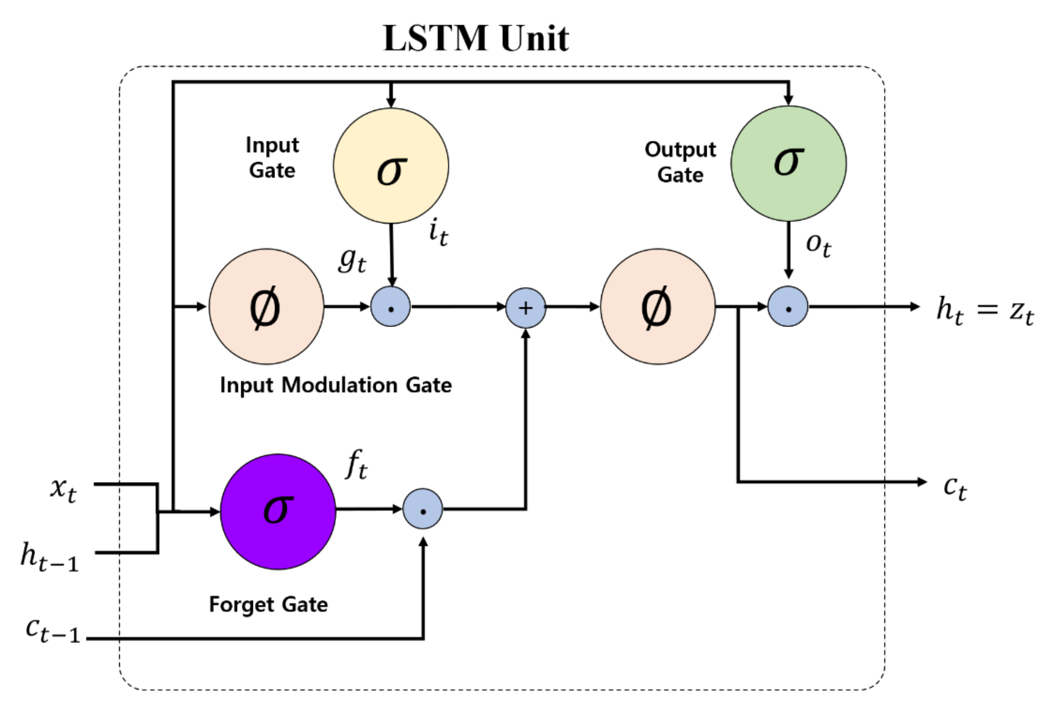
2.2. LSTM
2.3. Kernel Density Estimation
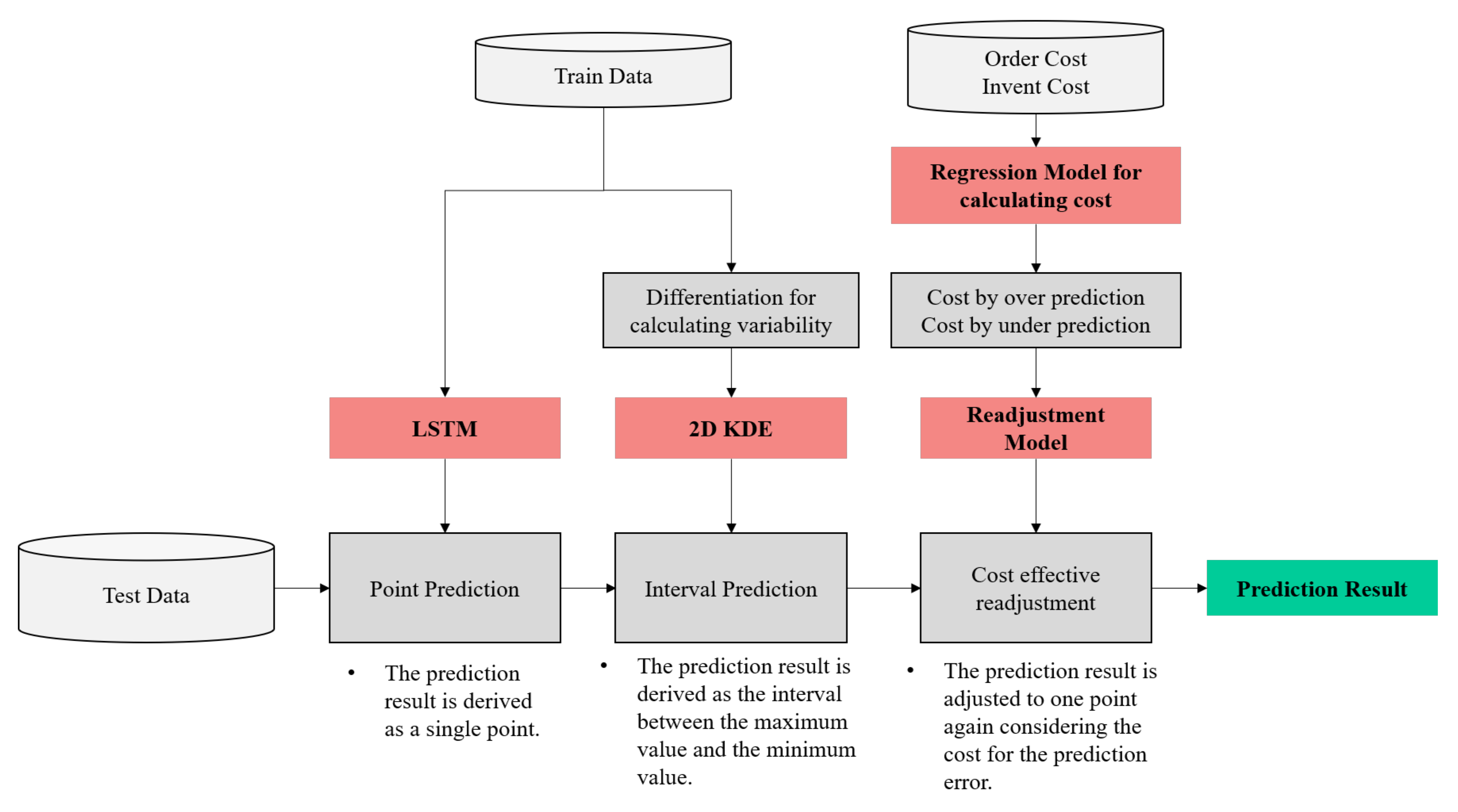
3. 2D KDE and LSTM-Based Forecasting Framework for Cost-Effective Inventory Forecasting
3.1. 2D KDE and LSTM-Based Prediction Algorithms for Inventory Forecasting
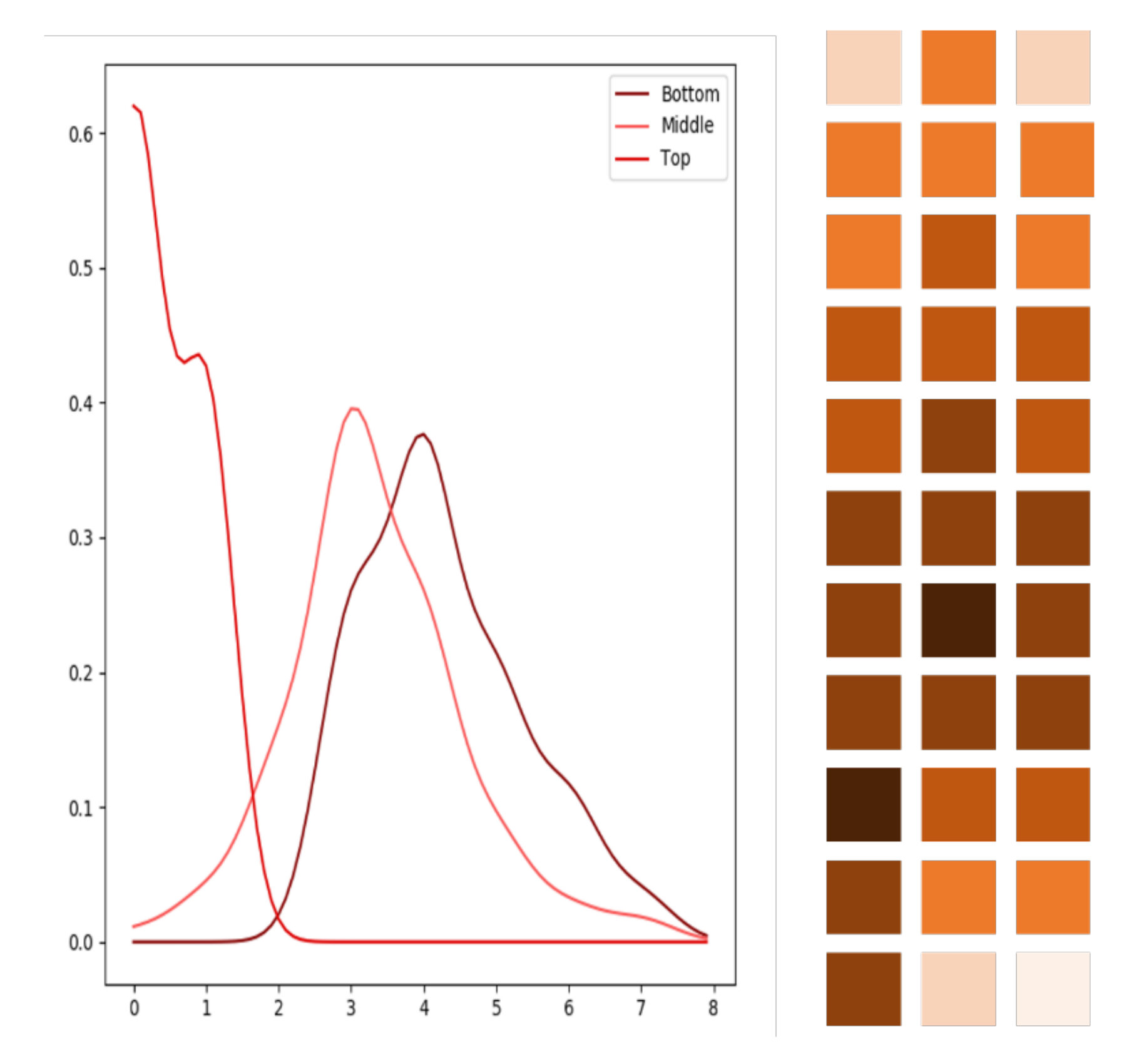
3.2. Interval Prediction by Means of 2D Kernel Density Estimation
| Algorithm 1 Creating 2D KDE map |
Input: rawData, smoothing rate, quanti Output: KDEmap, rawScale, diffScale
|
| Algorithm 2 CalcConfidenceInterval. |
Input: Predicted, KDEmap, confidencial rate, rawScale Output: Distance data, trainDistance, testDistance
|
3.3. Calculation of Adjusted Estimates Reflecting the Cost of Prediction Error
4. Performance Analysis
4.1. Experiment Design
4.2. Performance Accuracy Analysis
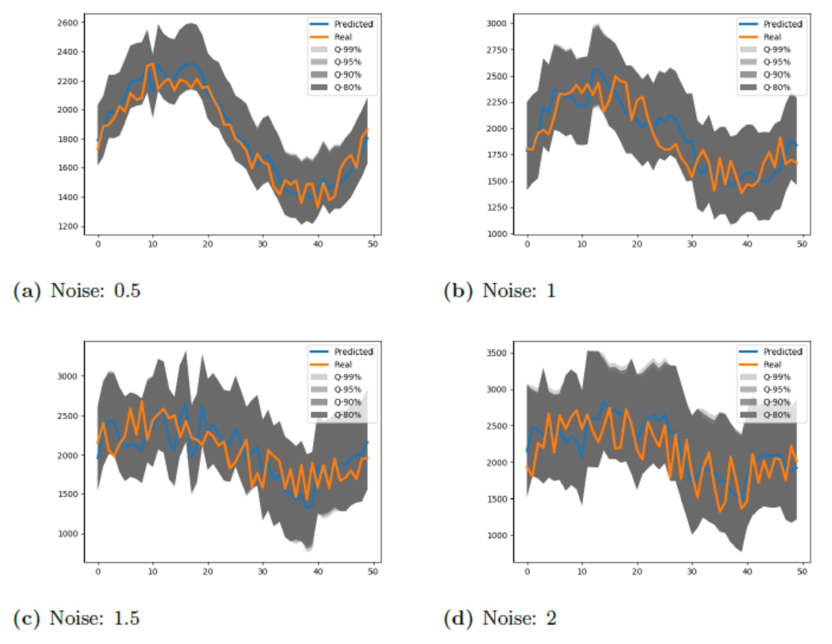
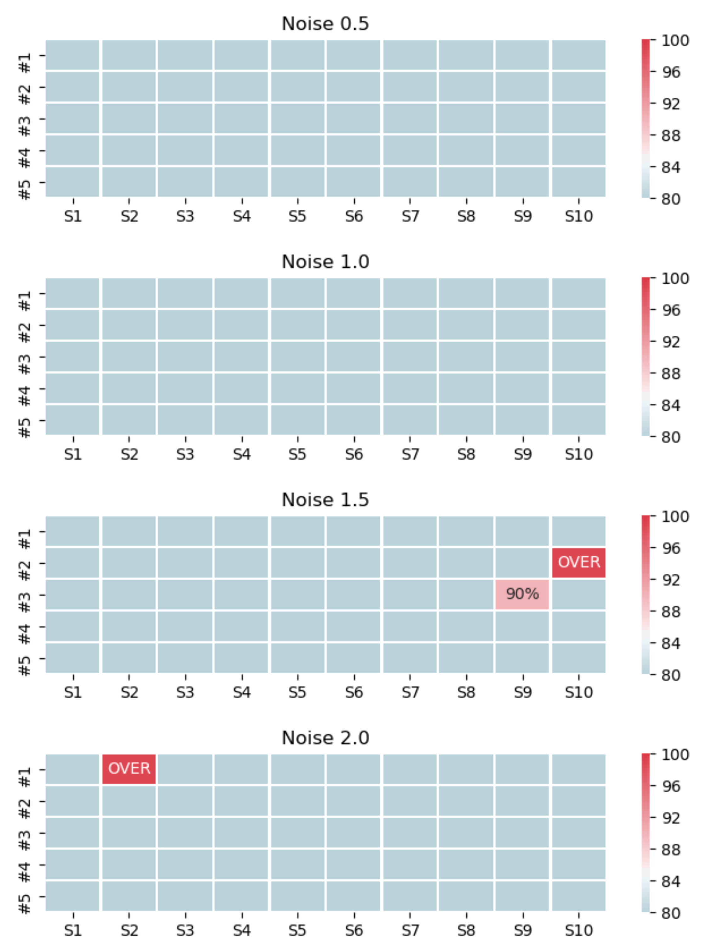
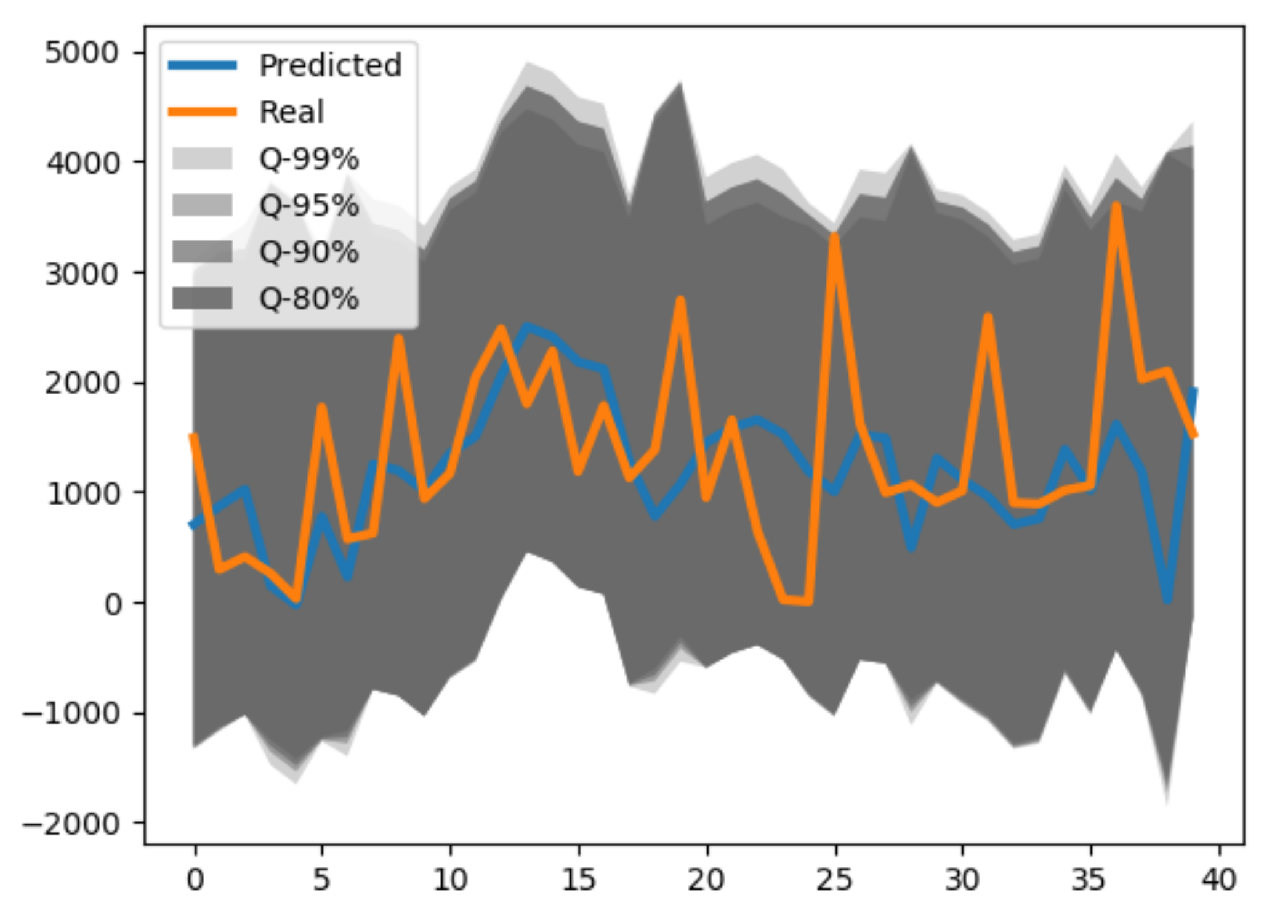
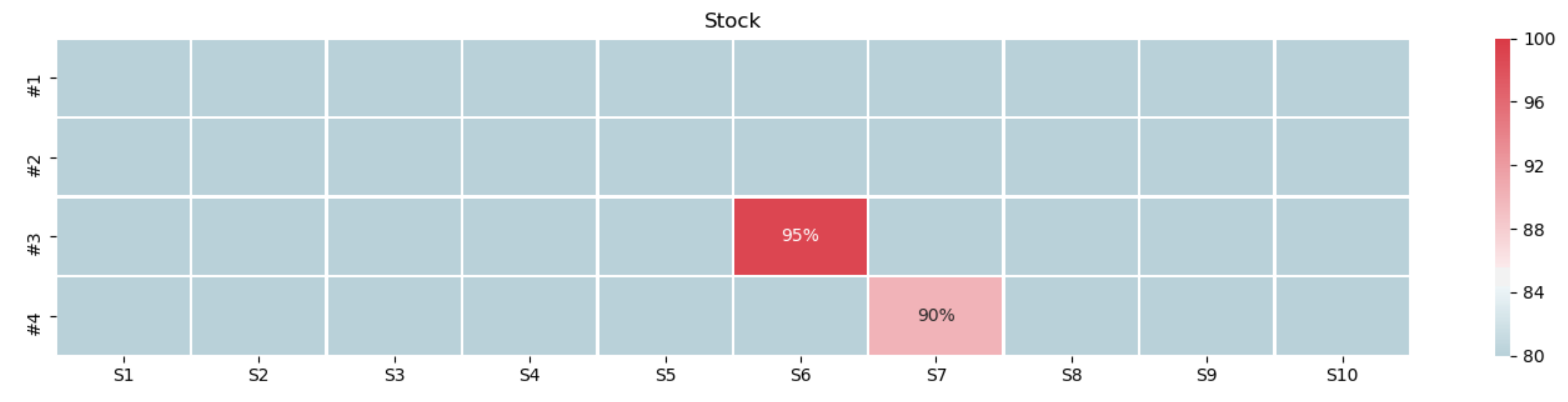
4.3. The Effect of Interval Prediction by 2D Kernel Density Estimation
4.4. Calculation of Cost Savings by Incorporating Forecasting Error Cost
5. Conclusions
Author Contributions
Funding
Institutional Review Board Statement
Informed Consent Statement
Data Availability Statement
Acknowledgments
Conflicts of Interest
References
- Fang, L.; Ma, K.; Li, R.; Wang, Z.; Shi, H. A statistical approach to estimate imbalance-induced energy losses for data-scarce low voltage networks. IEEE Trans. Power Syst. 2019, 34, 2825–2835. [Google Scholar] [CrossRef]
- Zhu, L.; Lu, C.; Dong, Z.Y.; Hong, C. Imbalance learning machine-based power system short-term voltage stability assessment. IEEE Trans. Ind. Inform. 2017, 13, 2533–2543. [Google Scholar] [CrossRef]
- Tang, C.; Wang, S.; Zhou, C.; Zheng, X.; Li, H.; Shi, X. An energy-image based multi-unit power load forecasting system. In Proceedings of the 2018 IEEE International Conference on Industrial Internet (ICII), Seattle, WA, USA, 21–23 October 2018; pp. 69–78. [Google Scholar]
- Bhattacharya, B.; Sinha, A. Intelligent fault analysis in electrical power grids. In Proceedings of the 2017 IEEE 29th International Conference on Tools with Artificial Intelligence (ICTAI), Boston, MA, USA, 6–8 November 2017; pp. 985–990. [Google Scholar]
- Wang, X.; Zhao, T.; Liu, H.; He, R. Power consumption predicting and anomaly detection based on long short-term memory neural network. In Proceedings of the 2019 IEEE 4th International Conference on Cloud Computing and Big Data Analysis (ICCCBDA), Chengdu, China, 12–15 April 2019; pp. 487–491. [Google Scholar]
- Helwig, N.; Pignanelli, E.; Schütze, A. Condition monitoring of a complex hydraulic system using multivariate statistics. In Proceedings of the 2015 IEEE International Instrumentation and Measurement Technology Conference (I2MTC), Pisa, Italy, 11–14 May 2015; pp. 210–215. [Google Scholar]
- Jiang, J.R.; Kuo, C.K. Enhancing Convolutional Neural Network Deep Learning for Remaining Useful Life Estimation in Smart Factory Applications. In Proceedings of the 2017 International Conference on Information, Communication and Engineering (ICICE), Xiamen, China, 17–20 November 2017; pp. 120–123. [Google Scholar]
- Chen, Z.; Liu, Y.; Liu, S. Mechanical state prediction based on LSTM neural netwok. In Proceedings of the 2017 36th Chinese Control Conference (CCC), Dalian, China, 26–28 July 2017; pp. 3876–3881. [Google Scholar]
- Zhang, W.; Guo, W.; Liu, X.; Liu, Y.; Zhou, J.; Li, B.; Yang, S. LSTM-based analysis of industrial IoT equipment. IEEE Access 2018, 6, 23551–23560. [Google Scholar] [CrossRef]
- Han, Q.; Liu, P.; Zhang, H.; Cai, Z. A wireless sensor network for monitoring environmental quality in the manufacturing industry. IEEE Access 2019, 7, 78108–78119. [Google Scholar] [CrossRef]
- Han, J.H.; Chi, S.Y. Consideration of manufacturing data to apply machine learning methods for predictive manufacturing. In Proceedings of the 2016 Eighth International Conference on Ubiquitous and Future Networks (ICUFN), Vienna, Austria, 5–8 July 2016; pp. 109–113. [Google Scholar]
- Lee, T.; Lee, K.B.; Kim, C.O. Performance of machine learning algorithms for class-imbalanced process fault detection problems. IEEE Trans. Semicond. Manuf. 2016, 29, 436–445. [Google Scholar] [CrossRef]
- Haddad, B.M.; Yang, S.; Karam, L.J.; Ye, J.; Patel, N.S.; Braun, M.W. Multifeature, sparse-based approach for defects detection and classification in semiconductor units. IEEE Trans. Autom. Sci. Eng. 2016, 15, 145–159. [Google Scholar] [CrossRef]
- Luo, Y.; Qiu, J.; Shi, C. Fault detection of permanent magnet synchronous motor based on deep learning method. In Proceedings of the 2018 21st International Conference on Electrical Machines and Systems (ICEMS), Jeju, Korea, 7–10 October 2018; pp. 699–703. [Google Scholar]
- Shi, H.; Bottieau, J.; Xu, M.; Li, R. Deep learning for household load forecasting-A novel pooling deep RNN. IEEE Trans. Smart Grid 2018, 9, 5271–5280. [Google Scholar] [CrossRef]
- Gan, D.; Wang, Y.; Zhang, N.; Zhu, W. Enhancing short-term probabilistic residential load forecasting with quantile long–short-term memory. J. Eng. 2017, 14, 2622–2627. [Google Scholar] [CrossRef]
- Toubeau, J.F.; Bottieau, J.; Vallée, F.; Grève, Z.D. Deep Learning-based Multivariate Probabilistic Forecasting for Short-Term Scheduling in Power Markets. IEEE Trans. Power Syst. 2018, 34, 1203–1215. [Google Scholar] [CrossRef]
- Tang, N.; Mao, S.; Wang, Y.; Nelms, R.M. Solar power generation forecasting with a LASSO-based approach. IEEE Internet Things J. 2018, 5, 1090–1099. [Google Scholar] [CrossRef]
- Wu, J.; Chan, C.K. The prediction of monthly average solar radiation with TDNN and ARIMA. In Proceedings of the 2012 11th International Conference on Machine Learning and Applications, Boca Raton, FL, USA, 12–15 December 2012; Volume 2, pp. 469–474. [Google Scholar]
- Hejase, H.A.; Assi, A.H. Time-series regression model for prediction of mean daily global solar radiation in Al-Ain, UAE. ISRN Renew. Energy 2012, 2012, 412471. [Google Scholar] [CrossRef] [Green Version]
- Muthusinghe, M.R.S.; Palliyaguru, S.T.; Weerakkody, W.A.N.D.; Saranga, A.M.H. Towards Smart Farming: Accurate Prediction of Paddy Harvest and Rice Demand. In Proceedings of the 2018 IEEE 6th Region 10 Humanitarian Technology Conference, Colombo, Sri Lanka, 6–8 December 2018; pp. 1–16. [Google Scholar]
- Chen, X. Prediction of urban water demand based on GA-SVM. In Proceedings of the 2009 ETP International Conference on Future Computer and Communication, Wuhan, China, 6–7 June 2009; Volume 14, pp. 285–288. [Google Scholar]
- Ai, S.; Chakravorty, A.; Rong, C. Household EV Charging Demand Prediction Using Machine and Ensemble Learning. In Proceedings of the IEEE International Conference on Energy Internet (ICEI), Southampton, UK, 27–29 September 2021; pp. 163–168. [Google Scholar]
- Zhu, M.; Zhang, J. Research of product oil demand forecast based on the combination forecast method. In Proceedings of the 2010 International Conference on E-Business and E-Government, Washington, DC, USA, 7–9 May 2010; pp. 796–798. [Google Scholar]
- Wang, Y.; Shen, Y.; Mao, S.; Chen, X.; Zou, H. LASSO and LSTM integrated temporal model for short-term solar intensity forecasting. IEEE Internet Things J. 2018, 6, 2933–2944. [Google Scholar] [CrossRef]
- LeCun, Y.; Bengio, Y.; Hinton, G. Deep learning. Nature 2015, 521, 436–444. [Google Scholar] [CrossRef] [PubMed]
- Wen, R.; Torkkola, K.; Narayanaswamy, B.; Madeka, D. A multi-horizon quantile recurrent forecaster. arXiv 2017, arXiv:1711.11053. [Google Scholar]
- Hochreiter, S.; Schmidhuber, J. Long short-term memory. Neural Comput. 1997, 9, 1735–1780. [Google Scholar] [CrossRef] [PubMed]
- Kharfan, M.; Chan, V.W.K.; Firdolas Efendigil, T. A data-driven forecasting approach for newly launched seasonal products by leveraging machine-learning approaches. Data Min. Decis. Anal. 2021, 303, 159–174. [Google Scholar]
- Gers, F. Learning to forget: Continual prediction with LSTM. In Proceedings of the 9th International Conference on Artificial Neural Networks: ICANN ’99, Edinburgh, UK, 7–10 September 1999; Volume 1999, pp. 850–855. [Google Scholar]
- Gers, F.A.; Schmidhuber, J.; Cummins, F. Learning to Forget: Continual Prediction with LSTM. Neural Comput. 2000, 12, 2451–2471. [Google Scholar] [CrossRef] [PubMed]
- Silverman, B.W. Density Estimation for Statistics and Data Analysis; Routledge: London, UK, 2018. [Google Scholar]
- Salinas, D.; Flunkert, V.; Gasthaus, J.; Januschowski, T. DeepAR: Probabilistic forecasting with autoregressive recurrent networks. Int. J. Forecast. 2020, 36, 1181–1191. [Google Scholar] [CrossRef]


| LSTM | units | 100 |
| return_sequence | True | |
| compile | loss function | root_mean_squared_error |
| Mean_absolute _percentage _error | ||
| optimizer | adam | |
| fit | nb_epoch | 1000 |
| batch_size | 4 | |
| verbose | 2 |
| Noise | 0.5 | |||||
| #1 | #2 | #3 | #4 | #5 | Average | |
| RMSE | 81.26246 | 117.6317 | 51.70315 | 82.43249 | 88.79546 | 84.36505 |
| MAPE | 3.498915 | 4.735661 | 2.440641 | 5.03232 | 5.401816 | 4.22187 |
| Noise | 1.0 | |||||
| #1 | #2 | #3 | #4 | #5 | Average | |
| RMSE | 139.8895 | 199.44 | 231.1574 | 173.0788 | 173.7208 | 183.4573 |
| MAPE | 5.077092 | 7.807049 | 11.14622 | 9.198444 | 8.848312 | 8.415424 |
| Noise | 1.5 | |||||
| #1 | #2 | #3 | #4 | #5 | Average | |
| RMSE | 320.0853 | 269.0784 | 262.721 | 269.6649 | 193.4566 | 263.0013 |
| MAPE | 11.6281 | 9.711254 | 11.57804 | 12.08087 | 10.46633 | 11.09292 |
| Noise | 2.0 | |||||
| #1 | #2 | #3 | #4 | #5 | Average | |
| RMSE | 317.9036 | 300.7283 | 335.1237 | 272.3147 | 228.4517 | 290.9044 |
| MAPE | 12.67522 | 10.22078 | 13.586 | 14.58546 | 10.63073 | 12.33964 |
| Warehousing Out | |||||
|---|---|---|---|---|---|
| #1 | #2 | #3 | #4 | Average | |
| RMSE | 653.9884 | 727.7047 | 1051.383 | 1094.891 | 881.992 |
| MAPE | 90.57324 | 32.43212 | 37.1611 | 37.0847 | 49.285 |
| RMSE | MAPE | |
|---|---|---|
| Linear | 1257.48 | 7.53 |
| Log | 1091.34 | 6.73 |
| Inverse | 1139.46 | 7.08 |
| Constant | 2000 | 3000 | 4000 | 6000 | 8000 | Average |
|---|---|---|---|---|---|---|
| #1 | ||||||
| 99% | 1,859,188 | 943,453 | 2,107,159 | 3,682,191 | 4,787,882 | 2,675,975 |
| 95% | 1,306,212 | 1,010,844 | 2,157,144 | 3,718,619 | 4,818,596 | 2,602,283 |
| 90% | 1,088,777 | 1,046,362 | 2,183,678 | 3,738,059 | 4,835,016 | 2,578,378 |
| 80% | 88,505 | 1,087,452 | 2,214,534 | 3,760,780 | 4,854,282 | 2,559,511 |
| #2 | ||||||
| 99% | −232,066 | 1,113,496 | 2,697,204 | 3,045,578 | 3,376,220 | 2,000,086 |
| 95% | 167,343 | 1,238,132 | 2,726,510 | 3,032,720 | 3,369,273 | 2,106,796 |
| 90% | 411,675 | 1,311,673 | 2,744,334 | 3,025,380 | 3,365,288 | 2,171,670 |
| 80% | 704,250 | 1,404,160 | 2,767,349 | 3,016,418 | 3,360,421 | 2,250,520 |
| #3 | ||||||
| 99% | −2,171,166 | 708,077 | 1,074,873 | 1,816,772 | 2,248,345 | 735,380 |
| 95% | −992,408 | 695,522 | 1,096,472 | 1,825,633 | 2,223,315 | 969,713 |
| 90% | −389,000 | 689,064 | 1,110,058 | 1,831,240 | 2,208,289 | 1,089,930 |
| 80% | 266,405 | 682,180 | 1,127,245 | 1,838,353 | 2,190,066 | 1,220,850 |
| #4 | ||||||
| 99% | 4,812,424 | 878,052 | 3,558,210 | 7,319,740 | 9,582,977 | 5,230,281 |
| 95% | 6,715,737 | 1,014,776 | 3,679,376 | 7,381,905 | 9,640,613 | 5,686,481 |
| 90% | 7,156,724 | 1,093,754 | 3,749,402 | 7,417,947 | 9,674,145 | 5,818,394 |
| 80% | 6,109,901 | 1,189,924 | 3,834,778 | 7,461,947 | 9,715,207 | 5,662,351 |
| Average | 1,730,906 | 1,006,684 | 2,426,770 | 3,994,580 | 5,015,621 | |
| #2, const | 2000 | 2010 |
|---|---|---|
| 99% | −232,066 | 34,466 |
| 95% | 167,343 | 455,022 |
| 90% | 411,675 | 691,177 |
| 80% | 704,250 | 970,307 |
| Minimum order quantity | 70 | |
| #3, const | 2060 | 2065 |
| 99% | −690,314 | 44,527 |
| 95% | 227,802 | 605,691 |
| 90% | 685,110 | 512,652 |
| 80% | 513,394 | 514,342 |
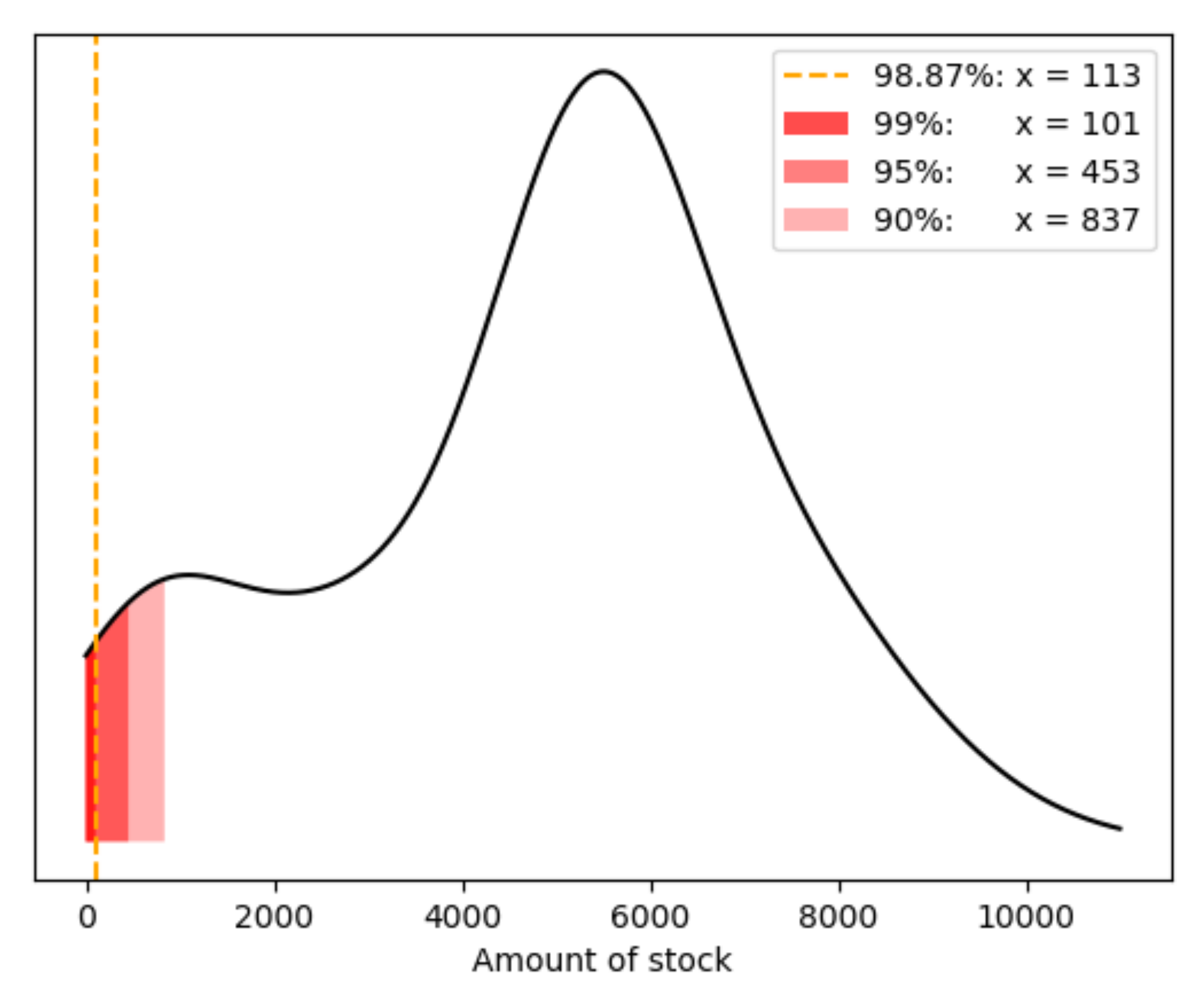
| Minimum order quantity | 113 | |
| Confidence interval 99% | 95% | 90% |
| Order amount 101 | 453 | 837 |
Publisher’s Note: MDPI stays neutral with regard to jurisdictional claims in published maps and institutional affiliations. |
© 2022 by the authors. Licensee MDPI, Basel, Switzerland. This article is an open access article distributed under the terms and conditions of the Creative Commons Attribution (CC BY) license (https://creativecommons.org/licenses/by/4.0/).
Share and Cite
Kim, M.; Lee, J.; Lee, C.; Jeong, J. Framework of 2D KDE and LSTM-Based Forecasting for Cost-Effective Inventory Management in Smart Manufacturing. Appl. Sci. 2022, 12, 2380. https://doi.org/10.3390/app12052380
Kim M, Lee J, Lee C, Jeong J. Framework of 2D KDE and LSTM-Based Forecasting for Cost-Effective Inventory Management in Smart Manufacturing. Applied Sciences. 2022; 12(5):2380. https://doi.org/10.3390/app12052380
Chicago/Turabian StyleKim, Myungsoo, Jaehyeong Lee, Chaegyu Lee, and Jongpil Jeong. 2022. "Framework of 2D KDE and LSTM-Based Forecasting for Cost-Effective Inventory Management in Smart Manufacturing" Applied Sciences 12, no. 5: 2380. https://doi.org/10.3390/app12052380
APA StyleKim, M., Lee, J., Lee, C., & Jeong, J. (2022). Framework of 2D KDE and LSTM-Based Forecasting for Cost-Effective Inventory Management in Smart Manufacturing. Applied Sciences, 12(5), 2380. https://doi.org/10.3390/app12052380