Article

Probabilistic Models for Competence Assessment in Education

by
Alejandra López de Aberasturi Gómez
*,
Jordi Sabater-Mir
and
Carles Sierra
*
Artificial Intelligence Research Institute (IIIA-CSIC), 08193 Barcelona, Spain
*
Authors to whom correspondence should be addressed.
Appl. Sci. 2022, 12(5), 2368; https://doi.org/10.3390/app12052368
Submission received: 15 December 2021 / Revised: 17 February 2022 / Accepted: 19 February 2022 / Published: 24 February 2022
(This article belongs to the Special Issue Women in Artificial intelligence (AI))

Abstract

:
Probabilistic models of competence assessment join the benefits of automation with human judgment. We start this paper by replicating two preexisting probabilistic models of peer assessment ( P G 1 -bias and PAAS). Despite the use that both make of probability theory, the approach of these models is radically different. While P G 1 -bias is purely Bayesian, PAAS models the evaluation process in a classroom as a multiagent system, where each actor relies on the judgment of others as long as their opinions coincide. To reconcile the benefits of Bayesian inference with the concept of trust posed in PAAS, we propose a third peer evaluation model that considers the correlations between any pair of peers who have evaluated someone in common: P G -bivariate. The rest of the paper is devoted to a comparison with synthetic data from these three models. We show that P G 1 -bias produces predictions with lower root mean squared error (RMSE) than P G -bivariate. However, both models display similar behaviors when assessing how to choose the next assignment to be graded by a peer, with an “ R M S E decreasing policy” reporting better results than a random policy. Fair comparisons among the three models show that P G 1 -bias makes the lowest error in situations of scarce ground truths. Nevertheless, once nearly 20 % of the teacher’s assessments are introduced, PAAS sometimes exceeds the quality of P G 1 -bias’ predictions by following an entropy minimization heuristic. P G -bivariate, our new proposal to reconcile PAAS’ trust-based approach with P G 1 -bias’ theoretical background, obtains a similar percentage of error values to those of the original models. Future work includes applying the models to real experimental data and exploring new heuristics to determine which teacher’s grade should be obtained next to minimize the overall error.

1. Introduction

Automated assessment and feedback of open-response assignments remain a challenge in computer science despite recent milestones in natural language processing. Competence assessment is a sensitive topic (current “AI Act” under discussion at the European Parliament pinpoints student assessment based on AI as high risk) with a clear impact on the certification of students as competent professionals and on their educational career progress.
Despite the efforts on opening the black box of neural networks, current neural models are rarely equipped with logical narratives of the decision chains that lead them to a final prediction or classification. Nevertheless, transparency and explainability are desirable requisites for automated assessment systems.
As a result, many researchers propose hybrid solutions combining the benefits of automation with human judgment. Specifically, they propose using peer assessments to help the teacher in the evaluation of students in large classrooms. Furthermore, numerous studies from the field of psychology point out that peer evaluation methods positively impact students’ formative process, leading toself-reflection [1,2,3].
Among the hybrid solutions in the bibliography, there are many that make use of Bayesian models to infer the grade of an assignment given a list of peer assessments ([4,5,6,7]). On the other hand, Gutierrez et al. [8] successfully built a network of trust among peers and the teacher that determines the relative importance that each peer’s opinion has in the computation of the assignment’s grade. This second approach, called PAAS, is very attractive as it exploits the naturalness with which a class of students evaluating each other can be modeled through multiagent theory.
The main objective of this article was to conceive a model that benefits from the Bayesian tradition in peer-assessment models while taking advantage of the concept of trust proposed by Gutierrez et al. [8]. As a result, we present P G -bivariate, a Bayesian model that translates the notion of trust among reviewers to a Bayesian approach thanks to its use of correlations among graders as the main feature to be learned by the model. Once P G -bivariate was implemented, we set out to compare it with one of the aforementioned Bayesian models and with PAAS in different experimental contexts. Given its theoretical robustness and the fact that it had been tested on an overwhelming number of more than 63,000 peers, the Bayesian model we chose to reimplement was P G 1 -bias [4].
The three models ( P G -bivariate, P G 1 -bias and PAAS) were then compared in the context of competency assessment. All of them use a probabilistic approach to estimate a probability distribution for each automatic grade. Their inputs are always peer assessments and a given percentage of the teacher’s grades (ground truths). Despite their commonalities, the relying idea varies for each model: whilst P G 1 -bias [4] and P G -bivariate are Bayesian network models, PAAS [8] applies multiagent system theory. More specifically, it is a competency assessment model: Given a community of agents and a human leader whose assessing criterion is to be mimicked, PAAS builds a matrix representing each agent’s trust in the rest.
The contributions of this work include (1) a Python reimplementation of PAAS, (2) a Python reimplementation of P G 1 -bias, (3) a new model that integrates PAAS’ use of trust measures with the Bayesian approach of P G -bivariate, and (4) a comparative analysis among the three models using simulated data and homogeneous units of measurement of the performance of the models.
This paper is structured as follows: In Section 1.2, we briefly review the concept of Bayesian network. After describing the materials and methods in Section 2, we present our models in Section 3. We experimentally evaluate the three models and compare them in Section 4. The discussion is presented in Section 4. Finally, we conclude in Section 5.

1.1. Related Work

The statistical models we present in this paper are part of a tradition of algorithms focused on score prediction. For instance, Bachrach et al. [6] makes use of a Bayesian model to grade tests. This model has two parts: a part that estimates the probability that a participant p will know the correct answer to a question q, represented by a variable c p q ; and a second part that models the probability of each potential answer r p q of participant p to question q as a variable that depends on the correct answer to question q, y q , and also on c p q .
On the other hand, Sterbini and Temperini [5] exploited peer-evaluation among students to support the teacher when grading open-answers. To do so, they represented each student as a triplet of discrete variables: knowledge, judgment, and correctness, which are interrelated. Each student is asked to choose the best of three peer answers, and her choice is influenced by the triplet representing the student. The correctness of the three peer answers presented to her also makes an impact on that choice.
De Alfaro and Shavlovsky [9] created a web-based tool for collaborative grading and evaluation of homework assignments. Similarly to our setup, students played in this platform both the role of graders and gradees. In addition, to encourage quality peer reviews, they made the final grade received by the students dependent on (i) the consensus grade computed for the student’s submission, (ii) an accuracy grade that measures the precision of the student in grading submissions, and (iii) a helpfulness grade that measures how helpful the reviews written by the student were. Such precision was computed by comparing the grades assigned by the student with the grades given to the same submissions by other students.
Perhaps more related to Piech et al. [4]’s work, Ashley and Goldin [10] devised a hierarchical Bayesian model to mine peer assessment data. However, although they do account for graders’ biases similarly to the models in this work, they mainly use the resulting posterior distribution over the conjoint parameter space to answer queries regarding the suitability of the employed rubric criteria.

1.2. Bayesian Networks

Conditional probability distributions allow decoupling of joint probability distributions into sequences of conditional probability distributions over lower-dimensional spaces and marginal probability distributions. This decomposition eases the reasoning about the model and allows to better incorporate domain expertise. The methodology that constructs joint probability distributions by applying the chain rule to conditional and marginal probability distributions is known as generative modeling (Figure 1).
Likewise, it is also possible to start with a coarse model represented by a joint probability distribution and then increase the complexity of the model by adding new variables as parents of that layer (Figure 2).
A joint distribution that factorizes into marginal and conditional distributions can be represented by a probabilistic graphical model (PGM). In particular, this section will introduce the fundamentals of Bayesian networks, a kind of PGM that will be used during the description of two from three of the probabilistic models implemented for this research.

1.3. Representation

A Bayesian network (BN) is a directed acyclic graph G = ( V , E ) and a set of parameters Θ = { θ 1 , θ 2 , , θ n } labeling the probability distributions associated with the nodes in the graph. This graph represents a decoupled joint probability distribution, such that
  • The vertices represent the random variables that we model.
  • For each vertex X i , there is a conditional probability distribution π ( X i | pa i ) .
The chain rule for Bayesian networks states that a Bayesian network M = ( G , Θ ) can be expressed as the product of marginal and conditional probability distributions associated to its nodes:
π M ( X ) = i = 1 n π ( X i | pa i ; Θ i )
where X = { X 1 , X 2 , , X n } and pa i stands for parent nodes and denotes the set of variables with a direct edge towards X i . The symbol Θ i represents the parameters of the probability distribution associated with that same vertex. If a node has no parents, then the probability distribution associated with it is marginal. As a side note, when depicting a Bayesian network, observed nodes will be shaded.
In addition, some representations will introduce the plate notation, a method of representing variables that repeat in a graphical model. Instead of drawing each repeated variable individually, a plate (rectangle) is used to group variables into a subgraph that repeat together, and a quantity is drawn on the plate to represent the number of times the subgraph repeats in the plate. It is assumed that the subgraph is duplicated that many times, the variables in the subgraph are indexed by the repetition number, and any links that cross a plate boundary are replicated once for each subgraph repetition.
Before deepening into the dependencies between variables in a Bayesian network, let us introduce some important concepts that will be used in the presentation of the models implemented in this research, namely parents, children, ancestors, ancestral ordering, and Markov blanket.
  • Given a node X in a Bayesian network, its parent nodes are the set of nodes with a direct edge towards X.
  • Given a node X in a Bayesian network, its children nodes are the set of nodes with an incoming edge from X.
  • Given a node X in a Bayesian network, its ancestors are given by the set of all variables from which we can reach X through a directed, arbitrarily long path.
  • Given the set of all the variables modeled in a Bayesian network, X = { X 1 , X 2 , , X N } , an ancestral ordering of the variables is followed when traversing the network; if every time we reach a variable X, we have already visited its ancestors.
  • Given a node X in a Bayesian network, its Markov blanket is given by its parents, its children, and the parents of its children.

1.4. Flow of Probabilistic Influence

The structure of a Bayesian network contains information regarding how variables in the model interact with each other. In other words, it is possible to determine whether the injection of information about a variable X updates our knowledge about another variable Y in the graph.
Considering the case of only two variables X and Y, if X is a parent of Y, then any update in the probability distribution associated with X will be reflected in changes in the probability distribution associated with Y. Likewise, knowing Y will update our information about X.
If we now think about three variables X , Y , W , three main situations can be distinguished:
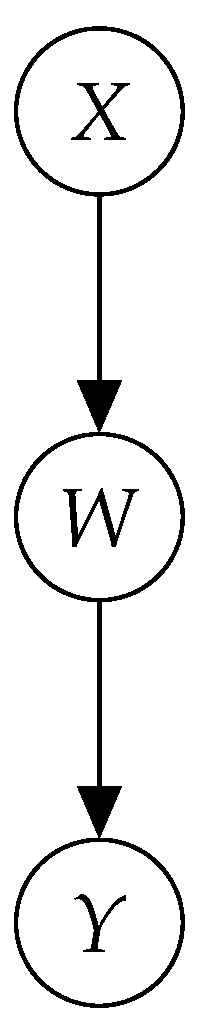
  • If W is an intermediate node and all the edges go in the same direction (Figure 3), then an update in X will be reflected in Y if and only if W is not an observed variable, and vice versa: an update in Y will be reflected in X if and only if W is not an observed variable.
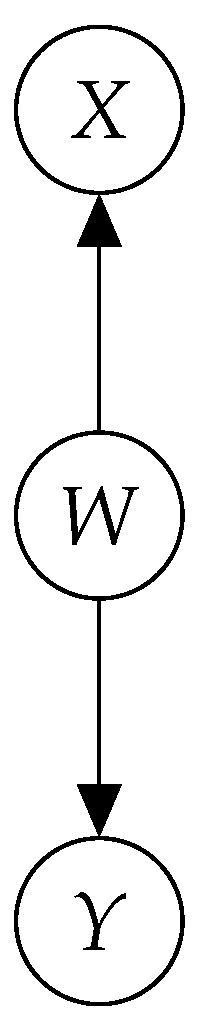
  • The same applies if W is a parent of two children X and Y (Figure 4). Again, there will be a flow of probabilistic influence from X to Y if and only if W is not observed.
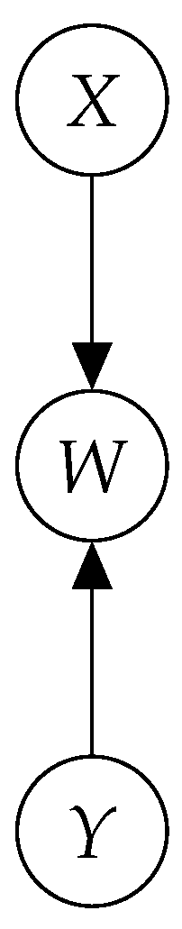
  • Finally, if X and Y are parents of W (v-structure, Figure 5), then the situation reverses, and there is a flow of probabilistic influence from X to Y if and only if W is observed.
In short, it can be stated that in Bayesian networks, influence flow is stopped by observed nodes and nonobserved v-structures. A v-structure is observed if W or any of its descendants is observed.
Formally, we say that there is a flow of probabilistic influence from X to Y if there is an active trail from X to Y, where an active trail is defined as follows:
  • Let G be a DAG.
  • Let X 1 X 2 be a trail in G .
  • A trail is active given a set of observed variables W if
    • Whenever there is a v-structure X i 1 X i X i + 1 , X i or one of its descendants is in W.
    • no other node along the trail is in W.
Let X, Y, and W be three disjoint sets of variables in G . W d-separates X from Y in G if X Y | W holds in G . X Y | W holds in G if there is no active trail between any variable in X and any variable in Y given W.
Given a variable X j and its Markov blanket, Mb j , for any set of variables X c ( V \ Mb j ) :
X c X j | Mb j
Hence, the Markov blanket of a variable in a BN d-separates that variable from the rest of the network.

2. Materials and Methods

All the analyses in this comparative study have been carried out with synthetic data. More specifically, for the generation of the data points injected into the Bayesian network models, ancestral sampling was used. According to this method, once a prior distribution π S ( θ ) and an observational model π S ( y ˜ | θ ) are specified, then we can iteratively generate an ensemble of reasonable model configurations and observations by sampling first from the prior
θ ˜ π S ( θ )
and then observations from the corresponding data generating process,
y ˜ π S ( y ˜ | θ ˜ )
Each simulated data point y ˜ adds an independent sample to the synthetic database. This database is then used as input for the model to fit. Please refer to Section 3 for further information about the parameters of the Bayesian network models presented in this paper. With regards to the non-Bayesian model (PAAS), its equivalence with the original Java implementation in Gutierrez et al. [8] was tested in Section 3.2.2. As for the data fed to it, we replicated the synthetic experiment presented in Gutierrez et al. [8] for a class of 50 students.

3. Results

3.1. Probabilistic Models of Peer Assessment

In the last decade, the boom of massive online courses (MOOCs) has propitiated that some platforms that provide online educational resources direct efforts towards implementing technologies that somehow automate the assessment process. The goal is to help teachers evaluate usually large numbers of assignments in this teaching modality.
The variability of answers to open questions and their challenges to natural language processing (NLP) techniques make automatic assessment a limited tool to deal with this task. The more unique or creative an assignment is, the less appropriate it is to rely on purely computer-based assessment methodologies [11]. Many authors have proposed peer assessment techniques as a promising alternative to speed up evaluation in online courses. Moreover, according to these voices, this methodology may provide other potential benefits such as helping students see the task from an assessor’s perspective and boosting self-reflection, as well as providing valuable feedback [3,12].
The three models of peer assessment that were studied in this paper are presented in this section. All of them are probabilistic and focus on an educational context and they all address a common question: How can we generate an automatic quality assessment of a submission not yet evaluated by the teacher in charge?

3.1.1. Personalized Automated Assessments

Provided a community (a class) and a leader or special member from that community (the teacher), the aim of Gutierrez et al. [8] is to predict as accurately as possible the personalized assessments that a teacher in a class would make. The key idea behind this model is to unequally weigh the opinion of the members in the community (the students) so that the closer a student’s marking style is to the teacher’s style, the more relevant that student’s opinion will be to predict the teacher’s opinion.
The closeness in marking styles will be represented as a trust value. That is, the teacher’s trust in a student depends on the similarity between the teacher’s (past) assessments and the student’s (past) assessments of the same assignments. In what follows, a one-to-one mapping between assessed students (a.k.a. gradees) and assignments is presumed. In other words, for all the experiments in this work, every student completed one and only one assignment (a.k.a. exam).
In the case there were no commonly assessed exams by the teacher and a given student, the authors propose a key concept: indirect trust. In short, an indirect trust measure is computed as the reputation of the student within the community, where this reputation is biased towards the teacher’s perspective.

Model

Let ε represent a person who needs to assess a set I of objects and let P be a set of peers able to assess objects in I . In the context of our analysis, this would be a teacher that wants to assess a number of assignments ( I ) completed by students that are evaluated by other students ( P ). Assessments made by peers v { ε } P on an object u I , noted z u v , are elements from an ordered evaluation space E .
An automated assessment of ε ’s opinion on an object u, noted e u ε , is a probability distribution P = { x 1 α 1 , x 2 α 2 , , x n α n } , where x i E and α i [ 0 , 1 ] , with i α i = 1 . A value α i represents the probability that ε ’s true assessment of u is x i . Hence, the more peaked the grading distribution on an object is, the more confident we will be that the automated assessment closely approaches ε ’s. Inversely, the flat, equiprobable distribution will be the one denoting ignorance of ε ’s true assessment.
Given a history of past peer assessments over u, O u , the ultimate goal of PAAS is to compute
P ( X u ε = x | O u )
That is, we aim to compute the probability distribution representing ε ’s evaluation on every object given the assessments of peers on that object.
To that end, every individual evaluation z u v from O u is taken into account, and the probability P ( X u ε = x | z u v ) is computed as a function of the trust (expected similarity between previous assessments) that ε has on v.
In our context, this trust is computed using the assignments graded in common by the teacher, i, and a student, j. In the case that there are no assignments in common, an indirect trust measure is obtained based on the notion of transitive trust: the trust that i has on student j can be computed from the trust i has on student k and the trust that student k has on student j. As there are many possible paths connecting i to j, appropriate aggregation functions have to be provided.

Direct Trust

When two agents i and j have commonly assessed one or more objects, a direct trust relationship between them T i , j can be computed. This direct trust is modeled as a probability distribution on the difference between the evaluations performed by i and j. This way, we keep information about whether j, for instance, underevaluates with respect to i, or overevaluates, or shows any other possible pattern. Information about their evaluation dissimilarities is summarized in that probability distribution.
The evaluation difference between two assessments performed by i and j is defined as
diff ( i , j ) = z u i z u j
If diff ( i , j ) > 0 , it follows from the above definition that agent i over rates u with respect to j. The opposite occurs if diff ( i , j ) < 0 .
From the previous definitions, it is clear that a situation of complete agreement between two agents is represented by
T i , j = { 0 1 }
In what follows, we will denote that situation as O .

Indirect Trust

If the leader has no objects assessed in common with a student j, a relation of indirect trust is computed. Since the model deals with probability distributions, it becomes necessary to define aggregation operators for probability distributions. These operators compute an indirect trust distribution from two trust distributions by combining differences in an additive way. The basic idea is that if the difference of opinions between k and j is x, and the difference of opinions between k and the teacher is y, then the difference of opinions between j and the teacher is x + y . Translating the above to probabilities and assuming independence of opinions, a combined distance distribution operator ⨂ can be defined as follows.
Definition 1. 
Given trust distributions  P  and  Q  over the numeric interval  [ b , b ]  we define their combined distance distribution, noted  R = P Q , as:
r ( X = x ) = x 1 + x 2 = x p ( X = x 1 ) q ( X = x 2 ) if x ( b , b ) x 1 + x 2 b p ( X = x 1 ) q ( X = x 2 ) if x b x 1 + x 2 b p ( X = x 1 ) q ( X = x 2 ) if x b
This aggregation combines the distributions along a path between two peers.
From that definition, it follows that ⨂ is commutative, and its neutral element is the probability distribution representing the complete agreement between two peers ( O ). In case there are several possible paths from the teacher to a student j, an aggregation operator ⨁ is defined to combine the aggregations computed along the different paths:
Definition 2. 
Given probability distributions P and Q over the numeric interval [ a , b ] , we define P Q , as
P Q = arg min T { P , Q } ( EMD ( T , O ) )
with EMD standing for Earth mover’s distance (a.k.a Wasserstein distance). (Informally, if the distributions are interpreted as two different ways of piling up a certain amount of dirt over the region D, the EMD is the minimum cost of turning one pile into the other, where the cost is assumed to be the amount of dirt moved times the distance by which it is moved [13]).
This aggregation is optimistically performed; it assumes that the combined distance that is closer to O (i.e., the one that brings the student’s and teacher’s opinions closer) is the true one. This operator is both commutative and associative. Thus, the order in which distributions (i.e., paths) are combined is irrelevant.

Incremental Updates

Every time an object is assessed by a peer, PAAS launches an overall update of the trust values and hence of the student marks. This update can be simplified as follows:
  • Initially, the default direct trust distribution T i , j between any two peers i and j is the one describing ignorance (i.e., the flat equiprobable distribution F ). When j evaluates an object α that was already assessed by i, T i , j is updated as follows:
  • Let P ( X u = x ) for x = diff ( i , j ) be the probability distribution of the assessment difference between i and j. The new assessment must be reflected in a change in the probability distribution. In particular, P ( X u = x ) is increased a fraction of the probability of X not being equal to x:
    P ( X u = x ) = P ( X u = x ) + γ · ( 1 P ( X u = x ) )
    For instance, if the probability of x is 0.6 and γ is 0.1, then the new probability of x becomes 0.6 + 0.1 × ( 1 0.6 ) = 0.64 . As in the example, the value of γ must be closer to 0 than to 1, for considerable changes can only be the result of information learned from the accumulation of many assessments.
  • The resulting T i , j is then normalized by computing the distribution that respects the new computed value and has a minimal relative entropy with the previous probability distributions:
    T i , j ( X ) = argmin P P ( X ) x p ( X α x ) log p ( X α x ) p ( X α x ) such that { p ( X α x ) = p ( X α x ) }
    where p ( X α x ) is a probability value in the original distribution, p ( X α x ) is a probability value in the potential new distribution P , and { p ( X α x ) = p ( X α x ) } specifies the constraint that needs to be satisfied by the resulting distribution.
    These direct trust distributions between peers are stored in a matrix C .
  • To encode the decrease in the integrity of information with time (information decays with time, I may be sure today about your high competence playing chess, but maybe in five years time I will be no longer sure if our interactions stop. You might have lost your abilities during that period), the direct trust distributions in C are decayed towards a decay limit distribution after a certain grace period. In our case, the limit distribution is the flat equiprobable F . When a new evaluation updates a direct trust distribution T i , j , T i , j is first decayed before it is modified.
  • The indirect trust distributions between ϵ and each peer are stored in a distributions vector t ε .
    Initially, t ε contains the probability distributions describing ignorance F . When matrix C is updated, t ε is also updated as a product of its former version times matrix C :
    t ϵ , j k + 1 = 0 < i n T i , j T ϵ , i k
  • If a direct trust distribution T ε , j exists between ε and j, the indirect trust distribution t ε , j is overwritten with T ε , j after the update of the indirect trust distributions.
Please notice that the decay in the direct distributions T i , j affects the indirect distributions t ε , j as well. This is because the indirect trust distributions are computed as aggregations of combinations of direct trusts.

3.1.2. Tuned Models of Peer Assessment in MOOCs

Looking for an answer to the same question posed by PAAS, the authors from Tuned Models of Peer Assessment in MOOCs [4] propose a Bayesian network model to represent the variables affecting the grade that a peer gives to another. Bayesian inference differentiates itself from other forms of inference by extending probability theory to the parameter space.
In this case, the space over which the probability is allocated is Z × Θ , where Z is the observational space and Θ is the parameter space. Observations are denoted as z u v Z , where u refers to the gradee and v to the grader. On the other hand, Θ is the space parameter.
More specifically, P G 1 -bias considers that z u v is influenced by the following:
  • The assignment’s true score, s u R . In the case of the implementation presented here, this is the teacher’s grade.
  • The grader’s bias, b v R . This bias reflects a grader’s tendency to either inflate or deflate their assessment by a certain number of percentage points. The lower these biases, the more accurate the grades will be.
  • The grader’s reliability, τ R , reflecting how close on average a grader’s peer assessments tend to land near the corresponding assignment’s true score after having corrected for bias. In this context, reliability is a synonym for precision or inverse variance of a normal distribution. Notice that the reliability of every grader is fixed to be the same value.
The posterior probability distribution is computed as the product of the prior over the parameters times the likelihood function evaluated on the observations (times a constant depending only on the observations):
π S ( s u , b v , τ | z u v ) Θ π S ( s u , b v , τ ) π S ( z u v | s u , b v , τ ) d θ
The authors propose that the prior distribution π S ( s u , b v , τ v ) can be decoupled into three marginal probability distributions:
π S ( s u , b v , τ ) = π S ( s u ) π S ( b v ) π S ( τ )
That is, the parameters are mutually independent. These priors have the form, according to Piech et al. [4], of
π S ( b v ) = N ( 0 , 1 η 0 )
π S ( s u ) = N ( μ 0 , 1 γ 0 )
π S ( τ ) = G 1 ( α 0 , β 0 )
Whereas the likelihood function is given by
π S ( z u v | s u , b v , τ ) = N ( s u + b v , 1 τ )
The resulting PGM is shown in Figure 6.

Partially Known Parameters

As Figure 6 shows, once the evidence z u v is injected, there is an active trail towards s v , which implies that we do not need an example of a teacher’s grade to make inference about how they would grade any student in the class. This active trail does not mean, however, that we are not allowed to introduce some ground truths grades s v in the Bayesian network. In that case, s v is said to be a partially known parameter, and its injection should result in a reduction of the variance of the posterior distribution. Half-shaded nodes represent partially known parameters in BNs.

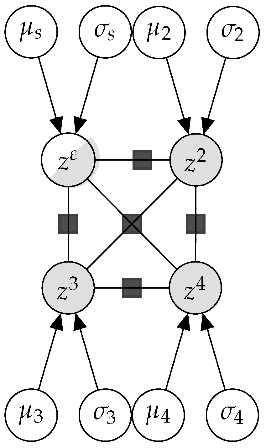
3.1.3. PG-Bivariate: A Bayesian Model of Grading Similarity

We contribute in this section with a novel Bayesian model of peer assessment, P G -bivariate. The approach adopted here tries to reconcile the benefits of Bayesian inference with the concept of trust posed in PAAS [8]. The key idea is to use a probability distribution to model the similarities as graders between any pair of peers in the system (teacher included). The chosen form for the probability density function modeling the similarities is a bivariate normal distribution. Figure 7 shows the graph representing the joint probability distribution of our model in a toy example with three students and a teacher, ϵ . The small, dark squares represent the relationship variables R between graders.
More specifically, consider a class with S students and a teacher ε . Each student v i assesses a number m i of peer students. The allocation of assignments to graders is such that every student is assessed by the same number n of peers. Denoting the assessments by peer v as z v , we wish to compute the grades that the teacher would give to each student, z ϵ . The model proposes that z v is sampled from a normal probability density function with parameters μ v and σ v . We could add complexity to the model and encode causal reasoning over these parameters by populating the layers above μ v and σ v . We limit, however, to this basic level of characterization, without adding any more variables influencing location or scale. Please notice that in this case, z are vector variables containing the assessments of each peer to her assigned reviewees. In the case of z ϵ , it is a partially known vector: making it a completely observed variable would imply that the teacher has assessed all the students in the class, which is not the case.
In line with the concept of direct trust coined by PAAS’ authors, we define a bivariate vector formed by the set of common assessments { ( z i v 1 , z i v 2 ) , ( z j v 1 , z j v 2 ) , , ( z k v 1 , z k v 2 ) } between two peers v 1 and v 2 , hereafter denoted as R v 1 , v 2 . This sequence is sampled from a bivariate normal distribution such that
  • The location vector, μ v 1 v 2 = ( μ v 1 , μ v 2 ) is composed of each of the peers’ location parameters separately.
  • The covariance matrix Σ v 1 v 2 contains the individual variances in its diagonal. The off-diagonal components codify the correlations between v 1 and v 2 when grading.
Putting it all together, the equations for P G -bivariate model are
z v i N ( μ v i , σ v i ) v i
R v i , v j N ( μ v i v j , Σ v i v j ) v i , v j
where μ v i v j = ( μ v i , μ v j ), Σ v i v j = σ v i 2 σ v i v j σ v i v j σ v j 2 , and ( v i , v j ) refers to a pair of graders having a set of evaluations in common.
We propose the following prior distributions for the hyperparameters:
σ v i Cauchy ( x 0 , γ )
μ v i N ( μ ¯ , σ ¯ )
As for the modeling of the covariance matrix Σ , denoting by D a diagonal matrix whose elements are the square root of the elements in the diagonal of Σ , D = D i a g ( Σ ) , then the correlation matrix Ω is related to the covariance matrix Σ by
Ω = D 1 Σ D 1
Stan offers correlation matrix distributions, which have support on the Cholesky factors of correlation matrices. Cholesky’s decomposition is unique: Given a correlation matrix Ω of dimension K, there is one, and only one, lower triangular matrix L such that L L T = Ω . We call such a matrix its Cholesky factor, and, according to Stan, even though models are usually conceptualized in terms of correlation matrices, it is better to operationalize them in terms of their Cholesky factors.
Hence, we used the prior
L LkjCorr ( η )
The observations in this system are vectors of peer grades z v , whereas the inference target is the vector of teacher grades, z ε = s . Please notice that in this case, no explicit mention is being made to the indirect trust. We limit our explicit modeling to the relationship between graders having a set of peers to assess in common. Nevertheless, from the graphical model, it can be seen that there exists a flow of probabilistic influence from any variable of type R to the rest of them. That is:, a change in the available information about the relationship between any pair of peers is reflected in an update of all the other variables R v i v j for all pairs { v i v j } , including those containing the professor. In turn, this directs the flow of probabilistic influence towards the parameters of the distribution from which R v i v j is sampled, namely μ v i v j and Σ v i v j .

Partially Known Parameters

Similarly to P G 1 -bias, P G -bivariate allows a flow of probabilistic influence from any peer’s grades to the teacher’s grading distribution without the need to have an example of how the teacher grades. However, it is possible to improve the inference results by introducing some of the teacher’s grades in the system. Hence, the components in s will be considered partially known parameters as well.

3.2. Experiments

The following results refer to synthetic databases, though future work includes applying the models to real data. Similar to in previous sections, the term ground truth is used here. In this context, ground truth is a synthetic data point with a known value that serves as input to the model.

3.2.1. Experiments on Bayesian Networks

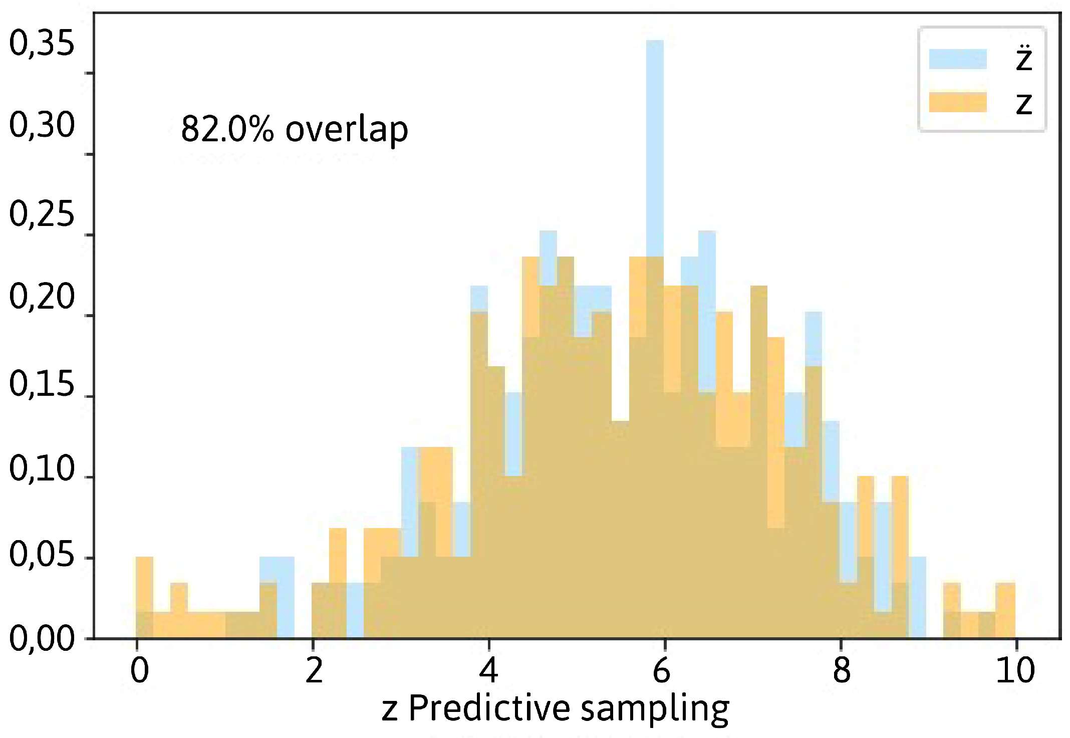
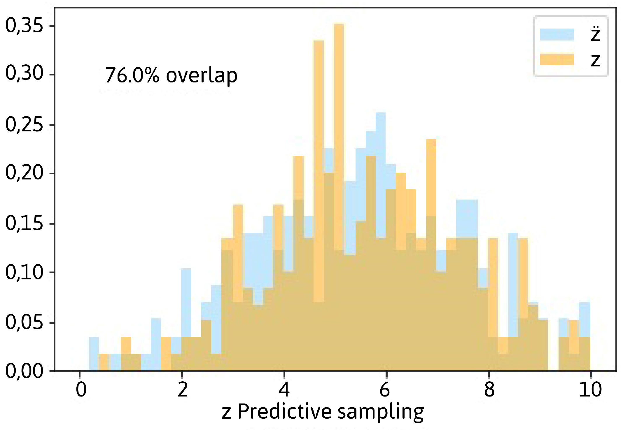
Posterior Predictive Sampling

Posterior predictive sampling (Equation (19)) is a useful method to compare predictions of new data based on past observations with the real data points. This comparison gives a sense of the estimations’ quality and may help during the tuning of the hyperparameters.
π S ( y | y ˜ ) = π S ( θ | y ˜ ) π S ( y | θ ) d θ
We sampled from the posterior predictive distribution of the two tested B N models, namely P G 1 -bias and P G -bivariate, comparing the histograms of predictions with the histogram of samples. Sampling from the posterior predictive distribution helped us calibrate the models’ hyperparameters for the prior distribution. In general, weakly informative and very weakly informative priors were proposed. However, we introduced some domain knowledge by centering the distributions of grades around positive numbers and restricting the variance parameters to only positive values, to name a couple of examples.
Recalling the prior distribution equation for model P G 1 -bias (Equation (10)), the chosen values in our implementation for ( α 0 , β 0 , γ 0 , η 0 , μ 0 ) were α 0 = 0.01 (very weak prior), β 0 = 0.01 (very weak prior), γ 0 = 10.0 (weak prior), η 0 = 1.0 , and μ 0 = 5.0 , whereas in the case of P G -bivariate, the chosen hyperparameters were x 0 = 0.0 (weak prior), γ = 0.25 (weak prior), μ ¯ = 5.0 , σ ¯ = 10.0 (weak prior), and η = 1.0 (weak prior).
Figure 8 represents a histogram of predicted peer grades z’s from the posterior predictive distribution in model P G 1 -bias for a class of 50 students (without ground truths). We observe the experimental histogram of observed peer grades in blue, z ˜ . The histogram of predictions (z) represents the distribution of data not part of the training set. This kind of prediction was repeatedly executed (20 times) to ensure that the results were consistent. Peer grades ranged from 0 to 10, following Equation (13).
We calculated the percentage overlapping between the histogram of samples and the histogram of predictions using the vector of elementwise minima [14]. The overlapping range was between 0 % (no overlap) and 100 % (identical distributions). On average, we observed an overlapping of 82 % . The range of values obtained for the overlapping in all the performed experiments was between 76 % and 84 % .
This value implies that the model captures the data generation system’s dynamics, which results in samples z that follow a very similar distribution to that from which z ˜ were sampled.
A similar figure to Figure 8 is obtained when we perform a posterior predictive sampling of the model presented in this paper, P G -bivariate. The overlapping, in this case, fell within the range [73–81%], with an average value of 77 % in 20 different runs (see Figure 9).
Although in this case, the model does not offer a causal explanation of the parameters μ v and σ v from the normal distribution governing z v (Equation (14)), the dynamics of the data generation system are captured. Intuitively, one would have expected a notably worse performance than P G 1 -bias for several reasons. First of all, P G 1 -bias models each use peer grade as a random variable that follows its normal distribution. On the other hand, the definition of the location parameter as the sum of the real grade and the graders’ bias allows a direct ascension of the flow of probabilistic influence towards s v . In the case of P G -bivariate, we adopt the perspective of a passive observer, representing the set of grades emitted by a referee as a random variable following a normal probability density function. Notice that in this case, no mention of who is evaluated by whom is being made. Hence, the location parameter μ v cannot be decoupled as in the former case to further ease the probabilistic influence flow.

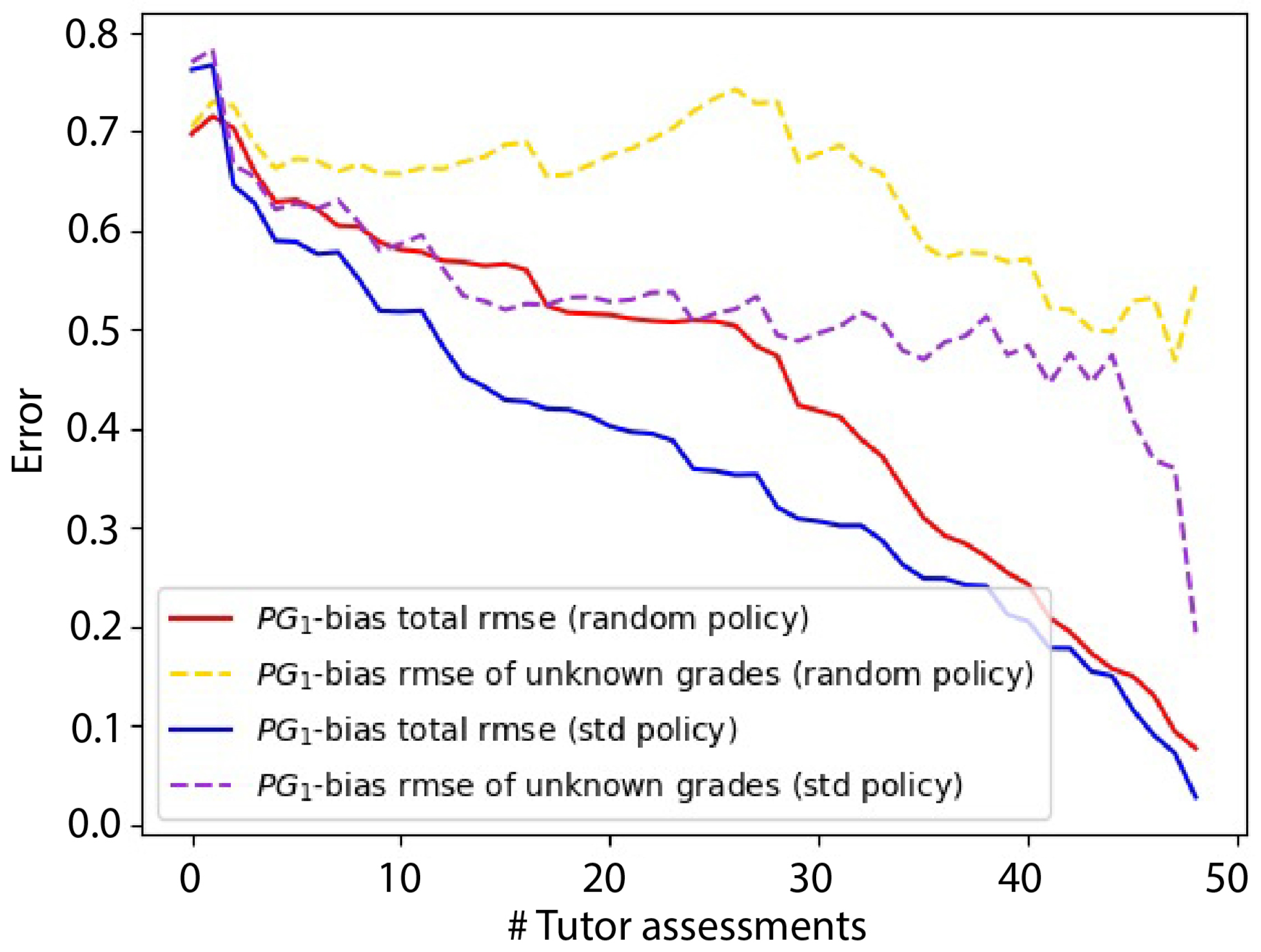
Studying the Error Evolution

To compare the performance of both models based on Bayesian networks, we studied the evolution of the models’ root mean squared error ( R M S E , Equation (20)) as a function of the number of observed true grades, keeping the number of students in a class, S, constant.
R M S E = 1 N n = 1 N ( y n y n ˜ ) 2
where y ˜ is the true value, y is the prediction, and N stands for the number of data points. Grades ranged from 0 to 10, both included. We examined the error evolution in both models as we introduced more teachers’ grades as ground truths. We assessed two different criteria to determine which new grade to introduce in each step of the loop:
  • Random choice (baseline): The next observed ground truth is chosen randomly.
  • Total R M S E decreasing policy: At each iteration, we picked and observed the true grade (i.e., the teacher’s grade) of that student whose assessment was introducing the highest root mean squared error.
As a result, we obtain four curves for each model:
  • The red line shows the evolution of the estimations’ R M S E as we introduce new ground truths following a random policy.
  • The yellow, discontinuous line shows the evolution of the estimations’ R M S E without considering the known ground truths to correct for overly optimistic low error values. Additionally, in this case, a random policy for ground truth injection is followed.
  • The blue line shows the evolution of the estimations’ R M S E as we introduce new ground truths following an R M S E decreasing policy.
  • The violet, discontinuous line shows the same information as the yellow line for the case of the R M S E decreasing policy.
Figure 10 shows the resulting four lines in the case of P G 1 -bias. Looking at the pair of continuous lines, we can see how R M S E falls as the number of known ground truths increases in all cases. As expected, computing the R M S E of all the grades (ground truths included) produces more optimistic errors. Moreover, it seems that the R M S E of the unknown grades (discontinuous lines) decreases much more slowly than for the continuous counterpart, that is, adding new ground truths does not reflect quickly on better quality of the predictions. According to Figure 6, introducing a ground truth s u has an impact on the bias b v of those peers v who have made an assessment of u: z u v . There is also a flow of probabilistic influence towards the grader’s reliability τ , which in the case of P G 1 -bias is common to all students. The informativeness of the prior determines the relative relevance that observed data and domain expertise have on the posterior distribution parameters. Hence, we believe that the choice of an informative prior over b v is preventing the model from showing an erratic behavior as new data is incorporated, but it also makes it more insensitive to the observations.
In general, the random policy yielded worse results for the discontinuous and continuous pairs of lines (red line showing higher error than the blue line, and yellow line showing higher error than the violet line).
We can see in Figure 11 the corresponding curves for P G -bivariate. In this case, the value of the R M S E was higher, which indicates that our predictions are, in general, worse than those of P G 1 -bias. We see again that the random policy yields worse results than the R M S E -decreasing policy (red line above blue line, and yellow line above violet line). As in the previous case, the slopes of the continuous lines are sharper than those of the discontinuous lines, which implies that the probabilistic influence from the observed teacher grades towards the predictions does not flow easily. The discontinuous lines also make it evident that when the number of grades we are computing the R M S E with is small (last portion of the graph), fluctuations of the R M S E increase.

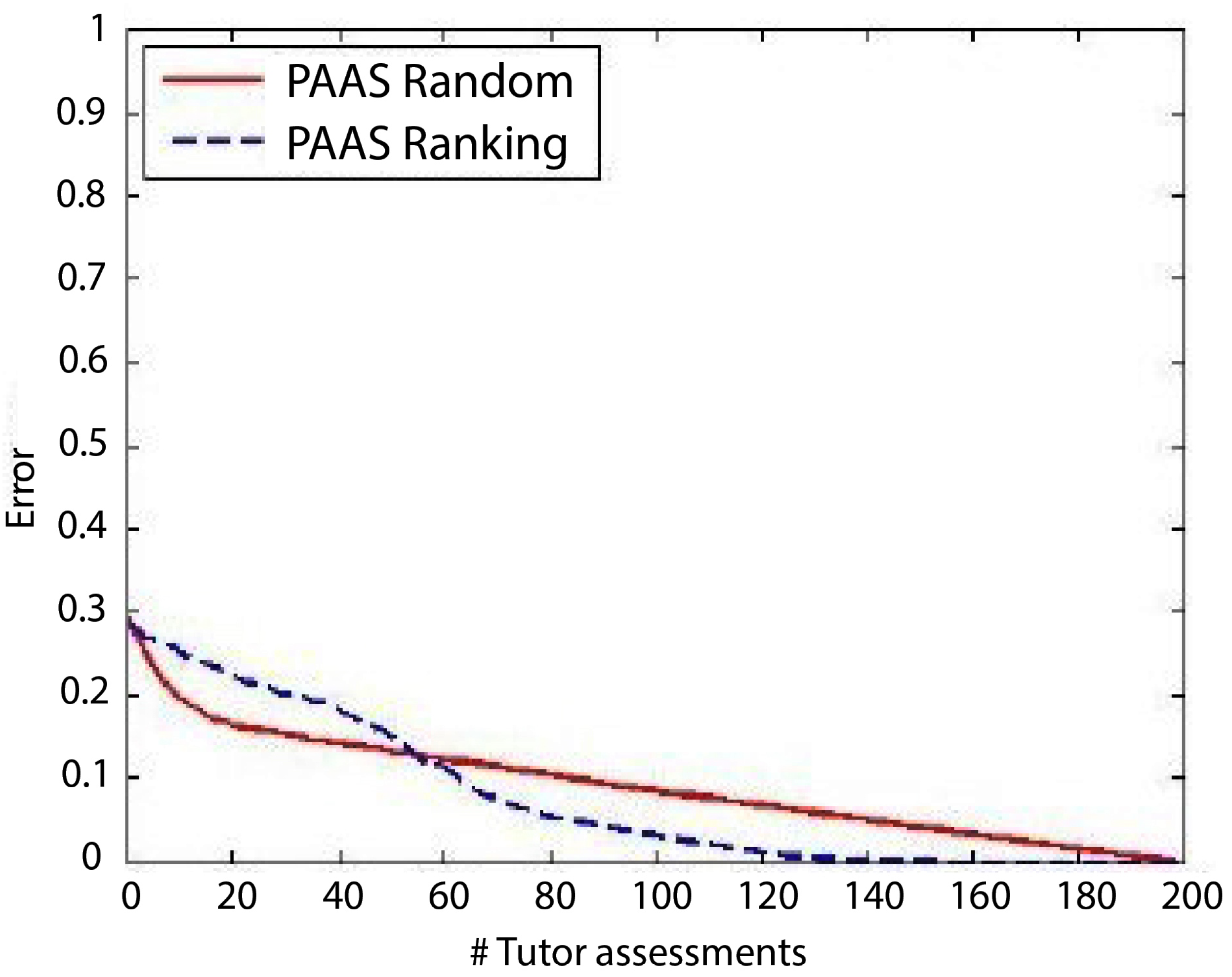
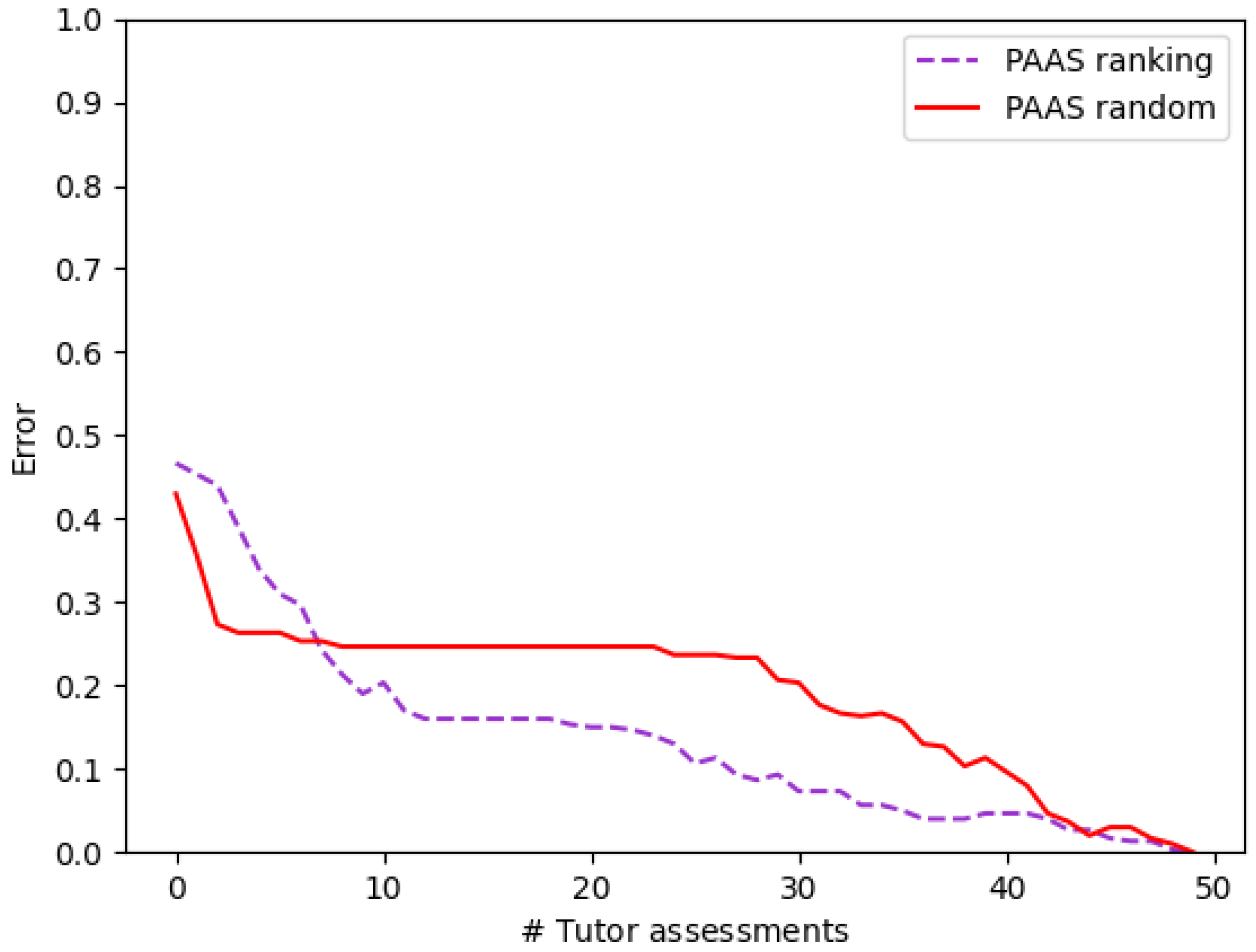
3.2.2. Experiments on PAAS

To make sure that PAAS software was being correctly implemented in Python, the synthetic experiment reported in Gutierrez et al. [8] was reproduced. We worked here under the premise that obtaining similar figures to the originals with our implementation would be a guarantee that the model functioning was being correctly replicated. This experiment consisted of a simulation of a classroom of 200 students with 200 submitted assignments, where each assignment was evaluated by 5 students (1000 peer assessments performed). In order to show a critical case, the authors simulated that half of the assignments were evaluated accurately by half of the students (that is, those students provided the same mark as the teacher), and the other half of the assignments were evaluated poorly (that is, randomly) by the rest of the class. In the simulation, they followed two policies to pick the next ground truth to observe as well. Such policies were a random one and another seeking to reduce the entropy of the grades by selecting the assignment with the highest entropy in its probability distribution, where entropy is computed as in information theory:
H ( P ( s u | { z u v } v S ) = s ˜ P ( s u = s ˜ | { z u v } v S ) · ln P ( s u = s ˜ | { z u v } v S )
The reported error line by Gutierrez et al. [8] is shown in Figure 12 (up). Down, we represent the obtained error for our implementation of PAAS in Python and a class of 50 students. We can see that although the original implementation shows a lower error for the first iterations, the behavior of both the original and our Python implementation is similar: both errors decrease as new ground truths are introduced in the system, and the entropy heuristic decreases the error faster than the random one. Furthermore, in both implementations, a crossing of the lines occurs when the number of observed ground truths is between 20 % and 30 % . From that point on, the performance of the heuristic-driven model is better.

3.2.3. Comparison of the Three Models

In order to compare the results, it was necessary that all of them were in the same unit. We adapted the B N models and computed their percentage of error to make comparisons (Equation (22)). This is the error function that will be represented in the following figures:
ϵ = Σ u S | s ˜ u s u | S
where S is the number of students, s ˜ u is the u’s true grade, and s u is the prediction. The experimental setups on which PAAS was tested considered quality assessments (that is, the graders were asked up to what degree, in their opinion, did an assignment meet a set of criteria). Although the model allowed both qualitative (e.g., { bad , good , excellent } ) or quantitative assessments, in the latter case, only integer grades were considered. Hence, for the comparisons to be fair, the Bayesian network models were adapted to predict integer grades ranging from 0 to 3 (both included). We ran this comparison mimicking the experimental arrangement described in the previous Section 3.2.2 for a synthetic class of 50 students.
Figure 13 shows the models’ comparison using the best policy of each of them. From all of them, P G 1 -bias keeps showing the lowest error when the number of known ground truths is small. Once past that region, both P G 1 -bias and P G -bivariate show similar shapes downwards, although P G 1 -bias keeps being solidly and continuously superior. Looking at PAAS’ results and despite its initial results being poor, we can see a sharp decrease in error once some evaluations were introduced as knowledge in the network, showing, from that point on, a similar, though fluctuating, performance to P G 1 -bias.

4. Discussion

The difficulties faced by neural models to make logical narratives of the decision chains that lead them to a final prediction pose a controversy on their applications in sensitive topics. One example is automatic grading and the ethical implications that it entails. These limitations have led the research to bet on hybrid solutions combining the benefits of automation with human judgment.
The first goal of this paper was to reproduce two models ( P G 1 -bias, by Piech et al. [4] and PAAS, by Gutierrez et al. [8]) of peer assessment. Both proposals estimate a probability distribution for each automatic grade using a probabilistic approach. These models’ inputs are peer assessments and a percentage of the teacher’s grades (ground truths). However, their theoretical foundations are different, and a common experimental setting was designed to make fair comparisons. All the code was written in Python, which implied the conversion of PAAS’ original code from Java and the familiarization with Stan’s Python interface (pystan) to reimplement P G 1 -bias.
Our second goal was to implement a model that combined the first’s powerful theoretical background with the second’s multiagent-based ideas. As a result, P G -bivariate translates the notion of trust among reviewers to a Bayesian approach thanks to its use of correlations among graders as the main feature to be learned by the model. This allows for the obtention of automatic grades of the same quality as those of P G 1 -bias without the need for complex causal reasoning over the distribution parameters representing each grader’s grading style.
Despite the similarities between previous literature and the algorithms presented here, some important distinctions should be noted: first, in contrast to the Bayesian model by Bachrach et al. [6], the variables considered in P G 1 -bias and P G -bivariate to predict the scores of the submitters are not only related to circumstances entailing the submitters, but also to the grades given by their peers and to the grading ability of such peers. Plus, instead of relying on highly abstract variables such as Sterbini and Temperini [5] do (e.g., judgment, knowledge), P G 1 -bias and P G -bivariate work with more traceable variables such as true scores and grader’s accuracy and reliability when correcting. Finally, and perhaps most importantly, all the algorithms in this work try to mimic the behavior that an expert would have had when faced with the task of grading a set of assignments. Hence, the trending opinion among peers is not what determines the quality of an assessment or what guides the prediction of an automatic score, in contrast to De Alfaro and Shavlovsky [9].
Regarding our experiments on Bayesian network models, the posterior predictive analysis showed that the distribution of new samples conditioned on the observed data was very similar to the distribution of samples. The posterior predictive distribution is influenced by the model configurations consistent with the relevant domain expertise and the observed data. This makes it ideal for informing predictions about future interactions with the latent system. Comparisons between the posterior predictive distribution and the observed data also measure how well our model approximates the latent system. Hence, we conclude that both models captured the data generating process.
When comparing these two models between them, specifically when analyzing the evolution of RMSE as a function of known ground truths (teacher’s grades), we can see that P G 1 -bias is slightly better. Not only does it report lower RMSE, but we observed that the computation times were shorter than in our model. According to the PyStan [15], most of the computation time during sampling with the NUTS algorithm is dedicated to calculating the Hamiltonian gradient. Looking at our computation times, P G -bivariate’s phase space has a more problematic surface to the sampler than that one of P G 1 -bias’. Hence, we conclude that although P G -bivariate uses a more simple definition of the distribution parameters (avoiding higher layers above μ v and σ v ), in this case, a higher abstraction might be desirable to reduce the number of parameters to fit. Regarding the higher RMSE values reported by our model, our hypothesis is that better and more informed choices of the hyperparameters will yield lower errors in the future, further facilitating the flow of probabilistic influence between variables. However, it is worth noting that P G -bivariate showed a similar behavior to P G 1 -bias in what policies are concerned: the random policy resulted in worse results than the one driven by the std error minimization policy. On the other hand, it is interesting to see that P G -bivariate offers remarkably good performance (the error of the predictions falls below 20 % when only 20 % of the ground truths are observed) despite its simplicity. The model can make predictions using the observed data and the correlations between graders, which somehow encode PAAS’s direct trust. The flow of probabilistic influence between these relationship variables behaves in this case as PAAS’ indirect trust. Given the success of PAAS in obtaining good automatic ratings, we find it interesting to continue exploring to what extent abstract variables can be dispensed within a Bayesian model that codifies the notion of trust between peers.
In Section 3.2.2, we showed that our Python implementation of PAAS, pyPAAS, reported a similar behavior to that by Gutierrez et al. [8]. To make fair comparisons among all models, we adapted the Bayesian inference models to compare with pyPAAS. More specifically, the synthetic data experiment was replicated for the three models. Under these conditions, P G 1 -bias and P G -bivariate reported similarly low errors in situations of scarce ground truths. From 10 % ground truths, the three models offer results of similar quality. It is worth mentioning that the calculation times for PAAS and our model were higher than those for P G 1 -bias when the class size started to become relatively large.
Throughout this research, synthetic data was used. Future work will apply the models to real experimental settings. Exploring new heuristics to determine which ground truth to observe next is also an exciting research line to continue this work.
Finally, regarding the robustness of our method, the simultaneous concurrence of three circumstances guarantees that the model is shielded from potential malicious coalitions:
  • The small number (5) of peers assessing each assignment.
  • The fact that these graders are chosen randomly.
  • The fact that the process is entirely anonymous concerning the students (the graders do not know who are they assessing, and the gradees do not know the identity of their graders).
In future work, we plan to identify the scenarios where each of these models is preferable. Specifically, it would be interesting to confirm the hypothesis that the two models P G -bivariate and PAAS (that implicitly penalize bad raters) perform better than P G 1 -bias under alliance and coalition dynamics among students. Applying the models to real experimental settings is also on the near horizon. Such settings may cover all those situations that can be modeled as consisting of multiple agents with different reputations issuing an opinion (e.g., peer review). Further improvements of P G -bivariate should find a point of compromise between the conceptual simplicity of the model and the number of parameters that it requires in exchange. Finally, exploring new heuristics to determine which ground truth to observe next is also an exciting research line to continue this work.

5. Conclusions

Our paper compares two state-of-the-art automatic evaluation methods ([4,8]) with a new model. This new model combines the Bayesian background of Piech et al. [4]’s with the use of a trust graph over the referees proposed by Gutierrez et al. [8]. As a result, we obtain a hierarchical Bayesian model that dispenses with the choice of abstract variables in favor of others that are easily interpretable. Similar to PAAS, this modeling through a trust graph explicitly shields the algorithm against bad graders.
There remain several issues to be addressed in future work. First, it is necessary to find a point of compromise between the conceptual simplicity of the model and the number of parameters that it requires in exchange for said simplicity. For example, in the case of P G -bivariate, dispensing with variables above the parameters μ s and σ s induces the necessity to calculate the parameters of all the bivariate distributions that describe correlations between students with some correction in common. This seems to cause a difficult phase space for the sampler because of the relatively long computation times. Second, we believe that further research that helps identify the scenarios where each of the compared models performs better is an interesting continuation line. For instance, it would be interesting to test whether the models that implicitly penalize bad raters perform better than P G 1 -bias under alliance and coalition dynamics among students.
Similar to other studies of the area ([5,6,8]), we find that following a greedy policy that maximizes the entropy reduction induced by new observations yields better predictions of the grades. Exploring new heuristics to determine which ground truth to observe next is also an exciting research line to continue this work.

Author Contributions

Conceptualization, A.L.d.A.G., J.S.-M. and C.S.; methodology, A.L.d.A.G., J.S.-M. and C.S.; software, A.L.d.A.G.; validation, A.L.d.A.G., J.S.-M. and C.S.; formal analysis, A.L.d.A.G., J.S.-M. and C.S.; investigation, A.L.d.A.G.; resources, J.S.-M. and C.S.; writing—original draft preparation, A.L.d.A.G.; writing—review and editing, J.S.-M. and C.S.; visualization, J.S.-M.; supervision, J.S.-M. and C.S.; project administration, C.S. All authors have read and agreed to the published version of the manuscript.

Funding

This research has been funded by ACCIO through the projects NanoMOOCs (COMRDI18-1-0010—RIS3CAT MEDIA), and ADDIA (ACE014/20/000039—INNOTEC) and by the CSIC through the project MARA (Intramural 202050E132). It has been funded also by the European Union Horizon 2020 FET Proactive projects “WeNet” (grant agreement Number 823783), “TAILOR” (grant agreement 952215) and “AI4EU” (grant agreement Number 825619).

Institutional Review Board Statement

Not applicable.

Informed Consent Statement

Not applicable.

Data Availability Statement

The models presented in this study are openly available in GitHub at https://github.com/aloaberasturi/Probabilistic-Models-of-Competency-Assessment (accessed on 14 December 2021).

Conflicts of Interest

The authors declare no conflict of interest.

Abbreviations

The following abbreviations are used in this manuscript:
AIArtificial intelligence
BNBayesian network
DAGDirected acyclic graph
MOOCMassive open online course
NLPNatural language processing
PAASPersonalized automated assessments
PGMProbabilistic graphical model
RMSERoot mean squared error

References

  1. Schön, D.A. The Design Studio: An Exploration of Its Traditions and Potentials; International Specialized Book Service Incorporated: London, UK, 1985. [Google Scholar]
  2. Tinapple, D.; Olson, L.; Sadauskas, J. CritViz: Web-based software supporting peer critique in large creative classrooms. Bull. IEEE Tech. Comm. Learn. Technol. 2013, 15, 29. [Google Scholar]
  3. Kulkarni, C.; Wei, K.P.; Le, H.; Chia, D.; Papadopoulos, K.; Cheng, J.; Koller, D.; Klemmer, S.R. Peer and self assessment in massive online classes. ACM Trans. Comput.-Hum. Interact. (TOCHI) 2013, 20, 1–31. [Google Scholar] [CrossRef] [Green Version]
  4. Piech, C.; Huang, J.; Chen, Z.; Do, C.; Ng, A.; Koller, D. Tuned models of peer assessment in MOOCs. arXiv 2013, arXiv:1307.2579. [Google Scholar]
  5. Sterbini, A.; Temperini, M. Correcting open-answer questionnaires through a Bayesian-network model of peer-based assessment. In Proceedings of the 2012 International Conference on Information Technology Based Higher Education and Training (ITHET), Istanbul, Turkey, 21–23 June 2012; pp. 1–6. [Google Scholar]
  6. Bachrach, Y.; Graepel, T.; Minka, T.; Guiver, J. How to grade a test without knowing the answers—A Bayesian graphical model for adaptive crowdsourcing and aptitude testing. arXiv 2012, arXiv:1206.6386. [Google Scholar]
  7. Mi, F.; Yeung, D.Y. Probabilistic graphical models for boosting cardinal and ordinal peer grading in MOOCs. In Proceedings of the AAAI Conference on Artificial Intelligence, Austin, TX, USA, 25–30 January 2015; Volume 29. [Google Scholar]
  8. Gutierrez, P.; Osman, N.; Roig, C.; Sierra, C. Personalised Automated Assessments. In Proceedings of the 2016 International Conference on Autonomous Agents & Multiagent Systems, Singapore, 9–13 May 2016; Jonker, C.M., Marsella, S., Thangarajah, J., Tuyls, K., Eds.; ACM: New York, NY, USA, 2016; pp. 1115–1123. [Google Scholar]
  9. De Alfaro, L.; Shavlovsky, M. CrowdGrader: A tool for crowdsourcing the evaluation of homework assignments. In Proceedings of the 45th ACM Technical Symposium on Computer Science Education, Atlanta, GA, USA, 5–8 March 2014; pp. 415–420. [Google Scholar]
  10. Ashley, K.; Goldin, I. Toward ai-enhanced computer-supported peer review in legal education. In Legal Knowledge and Information Systems; IOS Press: Amsterdam, The Netherlands, 2011; pp. 3–12. [Google Scholar]
  11. Balfour, S.P. Assessing Writing in MOOCs: Automated Essay Scoring and Calibrated Peer ReviewTM. Res. Pract. Assess. 2013, 8, 40–48. [Google Scholar]
  12. Admiraal, W.; Huisman, B.; Pilli, O. Assessment in Massive Open Online Courses. Electron. J. E-Learn. 2015, 13, 207–216. [Google Scholar]
  13. The Earth Mover’s Distance (EMD); The Stanford University: Stanford, CA, USA, 1999.
  14. Swain, M.J.; Ballard, D.H. Color indexing. Int. J. Comput. Vis. 1991, 7, 11–32. [Google Scholar] [CrossRef]
  15. Stan Development Team. PyStan: The Python Interface to Stan. 2021. Available online: http://mc-stan.org/2 (accessed on 14 December 2021).
Figure 1. Iterative addition of variables to a generative model. This methodology constructs a joint probability distribution from intermediate conditional probability distributions.
Applsci 12 02368 g001
Figure 2. Reverse construction of a joint probability distribution. In this case, we begin with a marginal distribution over some few variables and then increase the complexity by conditioning this distribution over a new set of (ancestor) nodes.
Applsci 12 02368 g002
Figure 3. Case 1.
Figure 3. Case 1.
Applsci 12 02368 g003
Figure 4. Case 2.
Figure 4. Case 2.
Applsci 12 02368 g004
Figure 5. Case 3.
Figure 5. Case 3.
Applsci 12 02368 g005
Figure 6. P G 1 -bias [4].
Applsci 12 02368 g006
Figure 7. P G -bivariate.
Applsci 12 02368 g007
Figure 8. Posterior predictive sampling from P G 1 -bias.
Applsci 12 02368 g008
Figure 9. Posterior predictive sampling from P G -bivariate.
Applsci 12 02368 g009
Figure 10. Reported R M S E for model P G 1 -bias.
Applsci 12 02368 g010
Figure 11. Reported R M S E for model P G -bivariate.
Applsci 12 02368 g011
Figure 12. Percentage error using random (red line) and entropy decreasing (violet, discontinuous line) assessment order as a function of the number of observed teacher’s grades for classes of 200 and 50 students using synthetic data. The upper figure represents the original implementation by Gutierrez et al. [8]. Below, our results are shown.
Applsci 12 02368 g012aApplsci 12 02368 g012b
Figure 13. Percentage error as a function of the number of observed ground truth grades reported by the three studied models.
Applsci 12 02368 g013
Publisher’s Note: MDPI stays neutral with regard to jurisdictional claims in published maps and institutional affiliations.

