Exact and Inexact Lifting Transformations of Nonlinear Dynamical Systems: Transfer Functions, Equivalence, and Complexity Reduction

Abstract

In this work, we deal with the problem of approximating and equivalently formulating generic nonlinear systems by means of specific classes thereof. Bilinear and quadratic-bilinear systems accomplish precisely this goal. Hence, by means of exact and inexact lifting transformations, we are able to reformulate the original nonlinear dynamics into a different, more simplified format. Additionally, we study the problem of complexity/model reduction of large-scale lifted models of nonlinear systems from data. The method under consideration is the Loewner framework, an established data-driven approach that requires samples of input–output mappings. The latter are known as generalized transfer functions, which are appropriately defined for both bilinear and quadratic-bilinear systems. We show connections between these mappings as well as between the matrices of reduced-order models. Finally, we illustrate the theoretical discussion with two numerical examples.

1. Introduction

Many problems from the applied sciences that involve a dynamic process under study, either to be solved, simulated, or even controlled, are described by models that could contain a considerable amount of variables and/or many inputs and outputs. This is particularly true in the context of fluid dynamics. For instance, equations, such as Navier–Stokes, Burgers’, or Kuramoto–Sivashinsky, are nonlinear partial differential equations (PDEs), which are complex and challenging to deal with by means of conventional/direct methods.

Thus, these equations are often discretized and linearized, resulting in linear ordinary differential equations (ODEs) described by a huge amount of states (internal variables). The large dimension results in high computational complexity, which leads to challenges in terms of simulation, analysis, and design. Consequently, there is a need to obtain a simplified model of smaller dimensions, which can still be used to provide accurate information for the simulation, analysis, and control of such systems.

Model reduction is commonly viewed as a methodology used for reducing the computational complexity of large scale complex models in numerical simulations. The goal is to construct a smaller system with the same structure and similar response characteristics as the original. For an overview of conventional model reduction methods, we refer the reader to the books [1,2,3]. For a fairly general overview on system-theoretical model order reduction (MOR) approaches, we refer the reader to [4]. In this work, we assume that the nonlinear systems to be modeled contains quadratic nonlinearities or it can be equivalently transformed to such a structure.

This class of systems is of interest since most smooth nonlinear systems can be exactly reformulated (lifted) as quadratic or quadratic-bilinear time-invariant systems (QBTIs), provided that the nonlinearities are analytical. Thus, even if the original model does not involve explicitly (only) quadratic nonlinearities, we could assume this structure (as we will see in the next sections). The main lifting approaches involve artificially introducing new variables into the state-space representation, computing derivatives, and rewriting all relations in the required format.

MOR methods specifically tailored for reducing QBTI systems have been proposed in [5,6,7,8]. Such approaches are fairly new, and most of them represent extensions of the techniques proposed for model reduction of linear time-invariant (LTI in short) systems and bilinear time-invariant (BTI) systems [9]. The latter class of systems represent a class of mildly nonlinear dynamical systems, which inherits many properties from LTIs; more specifically speaking, BTIs have many systems and control theoretical quantities that are very closely related or can be easily extended from LTIs (infinite Gramians, system norms, stability properties, etc.). Additionally, model reduction of BTIs is a fairly established sub-field of MOR that has been constantly developed in recent decades. We mention here the research endeavors [10,11,12,13,14] that preceded the more recent works in [15,16,17,18,19].

With an ever-increasing availability of measured data in many engineering fields, the need for incorporating measurements in the modeling process has steadily grown over recent decades. The main challenge lies in effectively using the available data in order to construct/learn models that can accurately represent the dynamics of the underlying dynamic process. Sometimes, in order to satisfy accuracy requirements, the fitted/learned models might have large dimensions and, hence, not be suitable for fast numerical simulation.

Thus, it is of interest to learn reliable reduced-order surrogate models to be used instead. Here, we assume that such models have particular dynamic structure, i.e., the nonlinearities include bilinear or quadratic-bilinear terms. As seen in the sequel, this is by no means restrictive. In recent years, many data-driven and learning methods have been designed specifically for the case of BTIs [20,21] and also for QBTIs [22,23,24,25,26]. Here, we mention another prolific method for learning models from data, the so-called dynamic mode decomposition (DMD) [27,28], which was recently extended to deal with BTIs in [29,30].

In this work, we cover a number of recent extensions of the data-driven non-intrusive method known in the MOR community as the Loewner framework (LF), originally introduced in [31]. We show various applications and connections between two prominent extensions of LF. Another goal of this work is to illustrate some properties and similarities of two established reformulation (lifting) strategies:

• Rewriting the dynamics of a generic nonlinear system (with analytic nonlinearities) into an equivalent form by enforcing quadratic-bilinear terms, and
• Approximating systems with quadratic-bilinear terms with bilinear systems by neglecting higher-order terms (such as cubic) from the power series expansion.

Lifting and reformulation strategies include classical approaches, such as the ones in [32,33], as well as more modern methods. Some of the latter were already used in connection to MOR applications, such as in [25,34,35]. In this work, by following such processes, we are able to establish connections between the generalized transfer functions (input–output mappings in the frequency domain) of the two classes of lifted systems (bilinear and quadratic-bilinear).

Additionally, we provide methods of connecting the reduced order models in bilinear format with the original matrices corresponding to the quadratic-bilinear (lifted) model. To the best of the author’s knowledge, connections, such as the ones mentioned above are indeed new and represent a fair share of this work’s novelty factor. Finally, we will show applications of the approaches under consideration for two benchmarks examples (a semi-discretized classical problem of computational fluid dynamics and a nonlinear electrical circuit).

2. Transforming the Original Dynamics to Quadratic or to Bilinear Format

This section discusses several methods for finding simplified or equivalent models for given complex nonlinear problems. Specifically, one requires approximated models written in matrix format (as state-space representation). Then, one could asses how well the approximation performs and how the equivalent model captures the inherent properties of the original, complex, and possibly large-scale nonlinear system. In this section, we present two important classes of methods, which yield reformulated systems with specific structures (bilinear and quadratic-bilinear). We will start with the former in what follows, which is based on truncating power series.

As the Taylor series expansion is used to approximate infinitely differentiable complex-valued functions around a particular expansion point, so do some of the methods presented in this section (for nonlinear systems). Since we require finite-dimensional models, a truncation is in order. This would be the first limitation as truncation automatically introduces an error. The other is that, in some cases, the approximation is usually good enough only around the expansion point but not very accurate in other regions. Finally, the dimensions of the rewritten system are much higher than those of the original nonlinear system (denoted here with n), e.g., polynomial growth in n.

The alternative is equivalently rewriting the dynamics involving analytic nonlinearities by adding variables and/or by computing derivatives. In doing so, it turns out that the reformulation is exact (no approximation is involved) and additionally, the increase in the dimensions of the rewritten system is linear in n. The downside is that this applies only to nonlinear functions with certain properties (however, in practical applications, many relevant cases are indeed covered).

Consider a nonlinear system described in state-space representation by the following system of differential equations:

$${\Sigma }_{\mathrm{N}}:\left\{\begin{array}{c}\dot{\mathbf{x}}\left(t\right)=\mathbf{f}\left(\mathbf{x}\left(t\right)\right)+\mathbf{g}\left(\mathbf{x}\left(t\right)\right)\mathbf{u}\left(t\right),\hfill \\ \mathbf{y}\left(t\right)=\mathbf{C}\mathbf{x}\left(t\right),\hfill \end{array}\right.$$

(1)

where $\mathbf{x}:\mathbb{R}\to {\mathbb{R}}^n$ is the state variable, $\mathbf{u}:\mathbb{R}\to \mathbb{R}$ is the control input, and $\mathbf{y}:\mathbb{R}\to \mathbb{R}$ is the observed output. Additionally, let $t⩾0,\mathbf{x}\left(0\right)={\mathbf{x}}_0$, and nonlinear vector-valued functions $\mathbf{f},\mathbf{g}:{\mathbb{R}}^n\to {\mathbb{R}}^n$ that are analytic in $\mathbf{x}$. For simplicity, assume that the output $\mathbf{y}$ depends linearly on the variable $\mathbf{x}$ (the more general case would be $\mathbf{y}\left(t\right)=\mathbf{h}\left(\mathbf{x}\right(t\left)\right)$ with $\mathbf{h}:{\mathbb{R}}^n\to {\mathbb{R}}^n$ also analytic in $\mathbf{x}$).

Without loss of generality, we assume that: $\mathbf{x}\left(0\right)=\mathbf{0},\mathbf{f}\left(\mathbf{x}\right(0\left)\right)=\mathbf{f}\left(0\right)=\mathbf{0}$. If this does not hold, set $\widehat{\mathbf{x}}\left(t\right)=\mathbf{x}\left(t\right)-{\mathbf{x}}_0\left(t\right)$ where ${\mathbf{x}}_0\left(t\right)$ is the zero input solution. Use the following notation $\widehat{\mathbf{f}}\left(\widehat{\mathbf{x}}\left(t\right)\right)=\mathbf{f}(\widehat{\mathbf{x}}\left(t\right)+{\mathbf{x}}_0\left(t\right))-\mathbf{f}\left({\mathbf{x}}_0\left(t\right)\right)$. Then, rewrite the system equations in terms of the new state:

$$\begin{array}{cc}\hfill \dot{\widehat{\mathbf{x}}}\left(t\right)& =\dot{\mathbf{x}}\left(t\right)-{\dot{\mathbf{x}}}_0\left(t\right)=\mathbf{f}\left(\mathbf{x}\left(t\right)\right)+\mathbf{g}\left(\mathbf{x}\left(t\right)\right)\mathbf{u}\left(t\right)-\mathbf{f}\left({\mathbf{x}}_0\left(t\right)\right)\hfill \\ & =\mathbf{f}(\widehat{\mathbf{x}}\left(t\right)+{\mathbf{x}}_0\left(t\right))-\mathbf{f}\left({\mathbf{x}}_0\left(t\right)\right)+\mathbf{g}\left(\mathbf{x}\left(t\right)\right)\mathbf{u}\left(t\right)=\widehat{\mathbf{f}}\left(\widehat{\mathbf{x}}\left(t\right)\right)+\mathbf{g}\left(\mathbf{x}\left(t\right)\right)\mathbf{u}\left(t\right),\hfill \end{array}$$

and also $\widehat{\mathbf{y}}\left(t\right)=\mathbf{C}(\widehat{\mathbf{x}}\left(t\right)+{\mathbf{x}}_0\left(t\right))$. Consequently, it follows that

$$\begin{array}{cc}\hfill \widehat{\mathbf{x}}\left(0\right)& =\mathbf{x}\left(0\right)-{\mathbf{x}}_0\left(0\right)=\mathbf{0},\widehat{\mathbf{f}}\left(\widehat{\mathbf{x}}\left(0\right)\right))=\widehat{\mathbf{f}}\left(0\right)=\mathbf{f}\left({\mathbf{x}}_0\right)-\mathbf{f}\left({\mathbf{x}}_0\right)=\mathbf{0}.\hfill \end{array}$$

Definition 1

([34]). The function $\mathbf{h}:\mathbb{R}\to \mathbb{R}$ is considered to be elementary if and only if it is a polynomial, rational, exponential, logarithmic, trigonometric, or root function or a composition of any of these classes of functions.

As mentioned in ([36]), there are a variety of practical applications where these kinds of elementary function appear

• ${\mathbf{h}}_1\left(x\right)=x_1^{{\alpha }_1}{x}_2^{{\alpha }_2}\cdots x_k^{{\alpha }_k}$, $\mathbf{x}={[x_1{x}_2\dots x_k]}^T$ in chemical rate equations, metal–oxide semiconductor field-effect transistor (MOSFET) in saturation mode.
• ${\mathbf{h}}_2\left(x\right)=\frac{x}{k+x}$ in chemical engineering, describing chemical rate equations or smoothing functions.
• ${\mathbf{h}}_3\left(x\right)=e^x$ in electronical circuit components, such as diodes or bipolar junction transistors.
• ${\mathbf{h}}_4\left(x\right)=sin\left(x\right)$ in control systems theory (where x is the angle used in steering of an object).

2.1. Bilinear Systems

We analyze bilinear time-invariant systems ${\Sigma }_{\mathrm{B}}=(\mathbf{C},\mathbf{E},\mathbf{A},\mathbf{N},\mathbf{B})$ characterized by the following equations:

$${\Sigma }_{\mathrm{B}}:\left\{\begin{array}{c}\mathbf{E}\dot{\mathbf{x}}\left(t\right)=\mathbf{A}\mathbf{x}\left(t\right)+\mathbf{N}\mathbf{x}\left(t\right)\mathbf{u}\left(t\right)+\mathbf{B}\mathbf{u}\left(t\right),\hfill \\ \mathbf{y}\left(t\right)=\mathbf{C}\mathbf{x}\left(t\right),\hfill \end{array}\right.$$

(2)

where $\mathbf{E},\mathbf{A},\mathbf{N}\in {\mathbb{R}}^{n\times n}$, $\mathbf{B}\in {\mathbb{R}}^{n\times m}$, $\mathbf{C}\in {\mathbb{R}}^{p\times n}$ and $\mathbf{x}\in {\mathbb{R}}^n$, $\mathbf{u},\mathbf{y}\in \mathbb{R}$. Here, we assume that the matrix $\mathbf{E}$ is invertible and can be incorporated in the other matrices appearing in the differential Equation (2) as:

$$\breve{\mathbf{A}}={\mathbf{E}}^{-1}\mathbf{A},\breve{\mathbf{N}}={\mathbf{E}}^{-1}\mathbf{N},\breve{\mathbf{B}}={\mathbf{E}}^{-1}\mathbf{B},\breve{\mathbf{E}}={\mathbf{I}}_n,$$

where ${\mathbf{I}}_n\in {\mathbb{R}}^{n\times n}$ denotes the identity matrix of length n. However, in practical scenarios in which the model is of large dimensions, we avoid explicitly computing the inverse of matrix $\mathbf{E}$, and incorporate it as above. That is why we will interchange the two (equivalent) representations throughout the paper.

For simplicity of exposition, we will treat the single-input, single-output (SISO) case. The multi-input multi-output case is indeed technically more involved; however, it is based on the same type of reasoning.

2.1.1. Carleman’s Linearization

In what follows, we introduce a well-established numerical tool that enforces approximating a nonlinear system with analytical nonlinearities be means of a bilinear system. The technique is commonly known as Carleman’s linearization and was originally introduced in [32]. Since this is an approximation technique, it follows that the bilinear system obtained is clearly not equivalent to the initial one (in terms of the input–output response). One main property of this method is that, as the dimension of the bilinear system increases, the original nonlinear system is better approximated. Of course, in many cases, one cannot overly increase the dimensionality, since this results in challenges, such as low computational time or depleted memory storage.

The Kronecker product of the internal state variable $\mathbf{x}={[x_1\cdots x_n]}^T$ with itself is defined as follows:

$$\mathbf{x}\otimes \mathbf{x}={[x_1^2{x}_1{x}_2\dots x_1{x}_n\dots x_n^2]}^T\in {\mathbb{R}}^{n^2}.$$

(3)

Denote the composition of k Kronecker products of the same vector $\mathbf{x}$ with itself with

$${\mathbf{x}}^{\left(k\right)}\left(t\right)=\mathbf{x}\left(t\right)\otimes \mathbf{x}\left(t\right)\otimes \dots \otimes \mathbf{x}\left(t\right)\in {\mathbb{R}}^{n^k},$$

(4)

where ${\mathbf{x}}^{\left(0\right)}=1,{\mathbf{x}}^{\left(1\right)}=\mathbf{x},{\mathbf{x}}^{\left(2\right)}=\mathbf{x}\otimes \mathbf{x}$ and ${\mathbf{x}}^{\left(j\right)}\otimes {\mathbf{x}}^{\left(k\right)}={\mathbf{x}}^{(j+k)},\forall j,k⩾1$. The infinite power series (Maclaurin series) expansions in $\mathbf{x}\left(t\right)$ for both functions $\mathbf{f}$ and $\mathbf{g}$ are written as follows:

$${\displaystyle \mathbf{f}\left(\mathbf{x}\left(t\right)\right)=\sum _{k=1}^{\infty }{\mathbf{F}}_k{\mathbf{x}}^{\left(k\right)}\left(t\right),\mathbf{g}\left(\mathbf{x}\right)\left(t\right)=\sum _{k=0}^{\infty }{\mathbf{G}}_k{\mathbf{x}}^{\left(k\right)}\left(t\right),}$$

(5)

where ${\mathbf{G}}_0\in {\mathbb{R}}^{n\times 1},{\mathbf{F}}_j,{\mathbf{G}}_j\in {\mathbb{R}}^{n^j\times n^j},j⩾1$. Here, ${\mathbf{F}}_1,{\mathbf{G}}_1$ denote the Jacobian matrices for $\mathbf{f}$ and $\mathbf{g}$, respectively. Moreover, ${\mathbf{F}}_2,{\mathbf{G}}_2$ denote the matrices containing the second-order derivatives (Hessian matrices), and so on (${\mathbf{F}}_k,{\mathbf{G}}_k$ denote the matrices containing the kth-order derivatives).

Now, by using a truncated version of the Maclaurin series of the functions by keeping only the first N terms for both series, where N represents the truncation index, we can write explicitly:

$$\left\{\begin{array}{c}\mathbf{f}\left(\mathbf{x}\right)=\sum _{k=1}^N{\mathbf{F}}_k{\mathbf{x}}^{\left(N\right)}={\mathbf{F}}_1\mathbf{x}+{\mathbf{F}}_2{\mathbf{x}}^{\left(2\right)}+\dots +{\mathbf{F}}_N{\mathbf{x}}^{\left(N\right)},\hfill \\ \mathbf{g}\left(\mathbf{x}\right)=\sum _{k=0}^{N-1}{\mathbf{G}}_k{\mathbf{x}}^{\left(k\right)}={\mathbf{G}}_0+{\mathbf{G}}_1\mathbf{x}+\dots +{\mathbf{G}}_{N-1}{\mathbf{x}}^{(N-1)}.\hfill \end{array}\right.$$

(6)

In the first equality in (6), we can neglect the term ${\mathbf{F}}_0$, without the loss of generality. This is usually chosen to be $\mathbf{0}$ in the case of non-existing forcing terms (and if indeed it is non-zero, it can be incorporated in the state vector by means of shifting). By substituting (6) into the state equation in (1), we write

$${\displaystyle \dot{\mathbf{x}}\left(t\right)=\sum _{k=1}^N{\mathbf{F}}_k{\mathbf{x}}^{\left(k\right)}\left(t\right)+\sum _{k=0}^{N-1}{\mathbf{G}}_k{\mathbf{x}}^{\left(k\right)}\left(t\right)\mathbf{u}\left(t\right).}$$

(7)

Hence, it follows that the left hand side of the differential equation in (7) contains the state variable vector $\mathbf{x}\left(t\right)$, while the right hand side contains various powers of it (${\mathbf{x}}^{\left(2\right)}\left(t\right),\dots ,{\mathbf{x}}^{\left(N\right)}\left(t\right)$). The strategy is to modify the state variable by adding higher-order terms that were missing; in this way, the dimension of the state vector increases. First, we compute the derivative of ${\mathbf{x}}^{\left(2\right)}\left(t\right)$ explicitly, as:

$$\begin{array}{cc}\hfill {\dot{\mathbf{x}}}^{\left(2\right)}\left(t\right)& =\frac{d{\mathbf{x}}^{\left(2\right)}\left(t\right)}{dt}=\frac{d\left(\mathbf{x}\right(t)\otimes \mathbf{x}(t\left)\right)}{dt}=\dot{\mathbf{x}}\left(t\right)\otimes \mathbf{x}\left(t\right)+\mathbf{x}\left(t\right)\otimes \dot{\mathbf{x}}\left(t\right)\hfill \\ & {\displaystyle =[\sum _{k=1}^N{\mathbf{F}}_k{\mathbf{x}}^{\left(k\right)}\left(t\right)+\sum _{k=0}^{N-1}{\mathbf{G}}_k{\mathbf{x}}^{\left(k\right)}\left(t\right)\mathbf{u}\left(t\right)]\otimes \mathbf{x}\left(t\right)}\hfill \\ & {\displaystyle +\mathbf{x}\left(t\right)\otimes [\sum _{k=1}^N{\mathbf{F}}_k{\mathbf{x}}^{\left(k\right)}\left(t\right)+\sum _{k=0}^{N-1}{\mathbf{G}}_k{\mathbf{x}}^{\left(k\right)}\left(t\right)\mathbf{u}\left(t\right)]}\hfill \\ & {\displaystyle =\sum _{k=1}^{N-1}[{\mathbf{F}}_k\otimes {\mathbf{I}}_n+{\mathbf{I}}_n\otimes {\mathbf{F}}_k]{\mathbf{x}}^{(k+1)}\left(t\right)+\sum _{k=0}^{N-2}[{\mathbf{G}}_k\otimes {\mathbf{I}}_n+{\mathbf{I}}_n\otimes {\mathbf{G}}_k]{\mathbf{x}}^{(k+1)}\left(t\right)\mathbf{u}\left(t\right).}\hfill \end{array}$$

We introduce the following summation of j terms, each containing $j-1$ Kronecker products, as follows (for $j⩾2$ and $k⩾1$)

$${\mathbf{F}}_{j,k}={\mathbf{F}}_k\otimes {\mathbf{I}}_n\otimes \dots \otimes {\mathbf{I}}_n+{\mathbf{I}}_n\otimes {\mathbf{F}}_k\otimes {\mathbf{I}}_n\otimes \dots \otimes {\mathbf{I}}_n+\dots +{\mathbf{I}}_n\otimes {\mathbf{I}}_n\otimes \dots \otimes {\mathbf{F}}_k,$$

where we set ${\mathbf{F}}_{1,k}:={\mathbf{F}}_k$, by definition. For example, the following formulas hold true:

$${\mathbf{F}}_{2,k}={\mathbf{F}}_k\otimes {\mathbf{I}}_n+{\mathbf{I}}_n\otimes {\mathbf{F}}_k,{\mathbf{F}}_{3,k}={\mathbf{F}}_k\otimes {\mathbf{I}}_n\otimes {\mathbf{I}}_n+{\mathbf{I}}_n\otimes {\mathbf{F}}_k\otimes {\mathbf{I}}_n+{\mathbf{I}}_n\otimes {\mathbf{I}}_n\otimes {\mathbf{F}}_k.$$

(8)

In a similar manner, define ${\mathbf{G}}_{j,k}$ for $j⩾1,k⩾0$. It follows that the time derivative of ${\mathbf{x}}^{\left(j\right)}\left(t\right)$ can indeed be written in terms of the newly defined matrices as:

$${\displaystyle {\dot{\mathbf{x}}}^{\left(j\right)}\left(t\right)=\sum _{k=1}^{N-j+1}{\mathbf{F}}_{j,k}{\mathbf{x}}^{(k+1)}\left(t\right)+\sum _{k=0}^{N-j}{\mathbf{G}}_{j,k}{\mathbf{x}}^{(k+1)}\left(t\right)\mathbf{u}\left(t\right),j⩾1.}$$

Increase the dimensions of the original state vector from n to $\mathcal{N}=n+n^2+\dots +n^N=\frac{n^N-n}{n-1}$, whereas n is the dimension of the original state variable $\mathbf{x}\left(t\right)$. In doing so, we also introduce a new state variable ${\mathbf{x}}^{\otimes }\left(t\right)$ defined as:

$$\begin{array}{c}\hfill {\mathbf{x}}^{\otimes }\left(t\right)={\left[\begin{array}{cccc}\mathbf{x}\left(t\right)& {\mathbf{x}}^{\left(2\right)}\left(t\right)& \dots & {\mathbf{x}}^{\left(N\right)}\left(t\right)\end{array}\right]}^T\in {\mathbb{R}}^{n^{\left(N\right)}}.\end{array}$$

(9)

By substituting the newly introduced notation in (9), we obtain a bilinear system with the following realization

$$\left\{\begin{array}{c}{\dot{\mathbf{x}}}^{\otimes }\left(t\right)={\mathbf{A}}^{\otimes }{\mathbf{x}}^{\otimes }\left(t\right)+{\mathbf{N}}^{\otimes }{\mathbf{x}}^{\otimes }\left(t\right)u\left(t\right)+{\mathbf{B}}^{\otimes }\mathbf{u}\left(t\right),\hfill \\ \mathbf{y}={\mathbf{C}}^{\otimes }{\mathbf{x}}^{\otimes }\left(t\right),\hfill \end{array}\right.$$

(10)

where ${\mathbf{x}}^{\otimes }\left(0\right)=\mathbf{0}$ and the matrices ${\mathbf{A}}^{\otimes },{\mathbf{N}}^{\otimes }\in {\mathbb{R}}^{\mathcal{N}\times \mathcal{N}},{\mathbf{B}}^{\otimes },({\mathbf{C}}^{\otimes }{)}^T\in {\mathbb{R}}^{\mathcal{N}}$ are as below:

$$\begin{array}{ccc}\hfill {\mathbf{A}}^{\otimes }& =& \left[\begin{array}{cccc}{\mathbf{F}}_{1,1}& {\mathbf{F}}_{1,2}& \dots & {\mathbf{F}}_{1,N}\\ \mathbf{0}& {\mathbf{F}}_{2,1}& \dots & {\mathbf{F}}_{2,N-1}\\ \mathbf{0}& \mathbf{0}& \ddots & {\mathbf{F}}_{3,N-2}\\ ⋮& ⋮& ⋮& ⋮\\ \mathbf{0}& \mathbf{0}& \dots & {\mathbf{F}}_{N,1}\end{array}\right],{\mathbf{N}}^{\otimes }=\left[\begin{array}{ccccc}{\mathbf{G}}_{1,1}& {\mathbf{G}}_{1,2}& \dots & {\mathbf{G}}_{1,N-1}& \mathbf{0}\\ {\mathbf{G}}_{2,0}& {\mathbf{G}}_{2,1}& \dots & {\mathbf{G}}_{2,N-2}& \mathbf{0}\\ \mathbf{0}& {\mathbf{G}}_{3,0}& \ddots & {\mathbf{G}}_{3,N-3}& \mathbf{0}\\ ⋮& ⋮& \ddots & ⋮& ⋮\\ \mathbf{0}& \mathbf{0}& \dots & {\mathbf{G}}_{N,0}& \mathbf{0}\end{array}\right],\hfill \\ \hfill {\mathbf{B}}^{\otimes }& =& \left[\begin{array}{cccc}{\mathbf{G}}_{10}& \mathbf{0}& \cdots & \mathbf{0}\end{array}\right],{\mathbf{C}}^{\otimes }=\left[\begin{array}{cccc}\mathbf{C}& \mathbf{0}& \cdots & \mathbf{0}\end{array}\right].\hfill \end{array}$$

This procedure involves approximation techniques (based on Taylor series expansion and truncation) to yield a BTI system that approximates the original system with generic nonlinearities. The main challenge with this method is that the dimensions of the derived bilinear system could be considerably higher than those of the original system. Indeed, by increasing the truncation index N will result in a better approximation. However, the increase in dimension of the bilinear system’s dimension $\mathcal{N}$ might yield serious memory storage problems (the storage of very large matrices). For many practical applications, one would restrict to low values of N, such as $N=2$ or $N=3$.

Example 1.

Consider a non-linear scalar system characterized by the equations:

$${\Sigma }_{\mathrm{N}0}:\left\{\begin{array}{c}\dot{x}\left(t\right)=-3x\left(t\right)+x\left(t\right)cos\left(x\right(t\left)\right)+u\left(t\right),\hfill \\ y\left(t\right)=2x\left(t\right).\hfill \end{array}\right.$$

Next, we use the Taylor series around the origin for the function $cos\left(x\left(t\right)\right)$

$$xcos\left(x\right(t\left)\right)=\sum _{k=1}^{\infty }{c}_k{x}^k\left(t\right)=x\left(t\right)-\frac{x^3\left(t\right)}{2!}+\frac{x^5\left(t\right)}{4!}-\dots ,c_k=\left\{\begin{array}{c}0,keven\hfill \\ \frac{{(-1)}^{(k-1)/2}}{(k-1)!},kodd\hfill \end{array}\right.,$$

and hence, write the differential equation as: $\dot{x}\left(t\right)=-2x\left(t\right)-{\sum }_{k=3}^{\infty }{c}_k{x}^k\left(t\right)+u\left(t\right).$ We identify the following values:

$$\begin{array}{cc}\hfill {\mathbf{F}}_{j,1}& =-2j,{\mathbf{F}}_{j,k}=\left\{\begin{array}{c}0,keven\hfill \\ j\frac{{(-1)}^{(k-1)/2}}{(k-1)!},kodd,k>1\hfill \end{array}\right.,\hfill \\ \hfill {\mathbf{G}}_{j,0}& =j,{\mathbf{G}}_{j,k}=0,j,k⩾1,{\mathbf{C}}_1=1,{\mathbf{C}}_h=0,h⩾2.\hfill \end{array}$$

First, we truncate at $N=3$ and by using that $x^{\left(k\right)}\left(t\right)=x^k\left(t\right)$, the new state variable is given by ${\mathbf{x}}_1^{\otimes }\left(t\right)={\left[\begin{array}{ccc}x\left(t\right)& x^2\left(t\right)& x^3\left(t\right)\end{array}\right]}^T\in {\mathbb{R}}^3$; the dynamics of the bilinear system corresponding to $N=3$ are written as

$${\dot{\mathbf{x}}}_1^{\otimes }\left(t\right)={\mathbf{A}}_1^{\otimes }{\mathbf{x}}_1^{\otimes }\left(t\right)+{\mathbf{N}}_1^{\otimes }{\mathbf{x}}_1^{\otimes }\left(t\right)u\left(t\right)+{\mathbf{B}}_1^{\otimes }u\left(t\right),y\left(t\right)={\mathbf{C}}_1^{\otimes }{\mathbf{x}}_1^{\otimes }\left(t\right),$$

with the system matrices computed as below:

$${\mathbf{A}}_1^{\otimes }=\left[\begin{array}{ccc}-2& 0& -\frac{1}{2!}\\ 0& -4& 0\\ 0& 0& -6\end{array}\right],{\mathbf{N}}_1^{\otimes }=\left[\begin{array}{ccc}0& 0& 0\\ 2& 0& 0\\ 0& 3& 0\end{array}\right],{\mathbf{B}}_1^{\otimes }=\left[\begin{array}{c}1\\ 0\\ 0\end{array}\right],{\mathbf{C}}_1^{\otimes }=\left[\begin{array}{ccc}2& 0& 0\end{array}\right].$$

Next, we increase the truncation index to $N=5$, i.e., ${\mathbf{x}}_2^{\otimes }\left(t\right)={\left[\begin{array}{cccc}x\left(t\right)& x^2\left(t\right)& \dots & x^5\left(t\right)\end{array}\right]}^T$ with ${\mathbf{x}}_2^{\otimes }\left(t\right)\in {\mathbb{R}}^5$. Hence, write the state and output equation as

$${\dot{\mathbf{x}}}_2^{\otimes }\left(t\right)={\mathbf{A}}_2^{\otimes }{\mathbf{x}}_2^{\otimes }\left(t\right)+{\mathbf{N}}_2^{\otimes }{\mathbf{x}}_2^{\otimes }\left(t\right)u\left(t\right)+{\mathbf{B}}_2^{\otimes }u\left(t\right),y\left(t\right)={\mathbf{C}}_2^{\otimes }{\mathbf{x}}_2^{\otimes }\left(t\right),$$

with the following system matrices:

$$\begin{array}{cc}\hfill {\mathbf{A}}_2^{\otimes }& =\left[\begin{array}{ccccc}-2& 0& -\frac{1}{2!}& 0& \frac{1}{4!}\\ 0& -4& 0& -\frac{2}{2!}& 0\\ 0& 0& -6& 0& -\frac{3}{2!}\\ 0& 0& 0& -8& 0\\ 0& 0& 0& 0& -10\end{array}\right],{\mathbf{N}}_2^{\otimes }=\left[\begin{array}{ccccc}0& 0& 0& 0& 0\\ 2& 0& 0& 0& 0\\ 0& 3& 0& 0& 0\\ 0& 0& 4& 0& 0\\ 0& 0& 0& 5& 0\end{array}\right],\hfill \end{array}$$

(11)

$$\begin{array}{cc}\hfill {\mathbf{B}}_2^{\otimes }& =\left[\begin{array}{c}1\\ 0\\ 0\\ 0\\ 0\end{array}\right],{\mathbf{C}}_2^{\otimes }=\left[\begin{array}{ccccc}2& 0& 0& 0& 0\end{array}\right].\hfill \end{array}$$

(12)

2.2. Quadratic-Bilinear Systems

We analyze QBTI systems ${\Sigma }_{\mathrm{QB}}=(\mathbf{E},\mathbf{A},\mathbf{Q},\mathbf{N},\mathbf{B},\mathbf{C})$ characterized by the following equations:

$$\begin{array}{c}\hfill {\Sigma }_{\mathrm{QB}}:\left\{\begin{array}{c}\mathbf{E}\dot{\mathbf{x}}\left(t\right)=\mathbf{A}\mathbf{x}\left(t\right)+\mathbf{Q}(\mathbf{x}\left(t\right)\otimes \mathbf{x}\left(t\right))+\mathbf{N}\mathbf{x}\left(t\right)\mathbf{u}\left(t\right)+\mathbf{B}\mathbf{u}\left(t\right),\hfill \\ \mathbf{y}\left(t\right)=\mathbf{C}\mathbf{x}\left(t\right),\hfill \end{array}\right.\end{array}$$

(13)

where $\mathbf{E},\mathbf{A},\mathbf{N}\in {\mathbb{R}}^{n\times n}$, $\mathbf{Q}\in {\mathbb{R}}^{n\times n^2}$, $\mathbf{B},{\mathbf{C}}^T\in {\mathbb{R}}^n$ and $\mathbf{x}\in {\mathbb{R}}^n$, $\mathbf{u},\mathbf{y}\in \mathbb{R}$.

For simplicity of exposition, we treat the single-input single-output (SISO) case. The multi-input multi-output (MIMO) case is technically more involved but it is based on similar ideas and procedural steps.

A strong argument for studying this problem is that a broad class of nonlinear systems can be written in quadratic-bilinear form by using exact transformations. These transformations can be applied to many different fields, e.g., fluid mechanic systems, electrical circuit models, and biochemical rate equations.

2.2.1. Reformulating Nonlinear Systems as QBTI Systems

Next, we mention a transformation that has been known in the literature as the McCormick relaxation [33]. The main result of it is that, by computing derivatives or by adding algebraic equations, the initial nonlinear system can be transformed into a QBTI system. The advantage of this method is that no approximation is performed: the quadratic-bilinear system is equivalent to the initial nonlinear system. The downside is that the procedure works only for certain types of smooth analytic nonliniarities. For application purposes, it works for some cases; however, nevertheless, one has to investigate the applicability of this method to its full extent.

Next, we acknowledge that an algorithm that implements lifting procedures in an automated way was explicitly formulated in [36]. As stated before, this is needed to equivalently transform a general nonlinear system into a QBTI system as in (13). It is to be noted that lifting strategies were already applied in various MOR-related works, such as [25,35].

As originally introduced in [36], one can distinguish two main strategies, i.e., by adding quadratic algebraic equations or by computing derivatives. The first procedure is seldom applicable by its own, and in most cases, one has to combine both of them. To show how the first approach works, we present a simple but self-explanatory example.

Example 2.

Start with the nonlinear differential equation $\dot{x}=x+x^3+u$. By introducing the new variable $z=x^2$, it follows that $\dot{x}=x+xz+u$, and hence the two are equivalent

$$\dot{x}=x+x^3+u\iff \left\{\begin{array}{c}\dot{x}=x+xz+u,\hfill \\ 0=z-x^2.\hfill \end{array}\right.$$

For the second category, we present a probative example that illustrates the lifting approach appropriately.

Example 3.

Consider the same nonlinear system as before, i.e.,

$$\begin{array}{c}\hfill {\Sigma }_{\mathrm{N}1}:\left\{\begin{array}{c}\dot{x}\left(t\right)=-3x\left(t\right)+x\left(t\right)cosx\left(t\right)+u\left(t\right),\hfill \\ y\left(t\right)=2x\left(t\right).\hfill \end{array}\right.\end{array}$$

(14)

By introducing two additional variables: $z\left(t\right)=sinx\left(t\right)$ and $w\left(t\right)=cosx\left(t\right)$, compute the time derivatives and then substitute the given terms

$$\begin{array}{c}\hfill \begin{array}{cc}\hfill \dot{x}\left(t\right)& =-3x\left(t\right)+x\left(t\right)w\left(t\right)+u\left(t\right),\hfill \\ \hfill \dot{z}\left(t\right)& =\dot{x}\left(t\right)cosx\left(t\right)=\left[-3x\left(t\right)+x\left(t\right)w\left(t\right)+u\left(t\right)\right]w\left(t\right),\hfill \\ \hfill & =-3x\left(t\right)w\left(t\right)+x\left(t\right)w^2\left(t\right)+w\left(t\right)u\left(t\right),\hfill \\ \hfill \dot{w}\left(t\right)& =-\dot{x\left(t\right)}sinx\left(t\right)=-\left[-3x\left(t\right)+x\left(t\right)w\left(t\right)+u\left(t\right)\right]z\left(t\right)\hfill \\ \hfill & =3x\left(t\right)z\left(t\right)-x\left(t\right)z\left(t\right)w\left(t\right)-z\left(t\right)u\left(t\right).\hfill \end{array}\end{array}$$

(15)

We managed to equivalently rewrite the original nonlinear system as a polynomial system but with cubical nonlinearities as can be observed in (15). However, there is one more step until the transformation to QBTI format is completed. We need to choose another two surrogate variables, i.e., $p\left(t\right)=x\left(t\right)z\left(t\right)$ and $r\left(t\right)=x\left(t\right)w\left(t\right)$, to be able to equivalently rewrite the above CTI (cubic time-invariant) system as a QBTI system. Hence, by substituting the new variables into (15), we can re-write the differential equations as:

$$\begin{array}{c}\hfill \begin{array}{cc}\hfill \dot{x}\left(t\right)& =-3x\left(t\right)+r\left(t\right)+u\left(t\right),\hfill \\ \hfill \dot{z}\left(t\right)& =-3r\left(t\right)+r\left(t\right)w\left(t\right)+w\left(t\right)u\left(t\right),\hfill \\ \hfill \dot{w}\left(t\right)& =3p\left(t\right)-p\left(t\right)w\left(t\right)-z\left(t\right)u\left(t\right).\hfill \end{array}\end{array}$$

(16)

Then, the next step is to explicitly compute the derivatives of the two new variables $p\left(t\right)$ and $r\left(t\right)$ as:

$$\begin{array}{c}\hfill \begin{array}{cc}\hfill \dot{p}\left(t\right)& =\dot{x}\left(t\right)z\left(t\right)+x\left(t\right)\dot{z}\left(t\right)\hfill \\ \hfill & =\left[-3x\left(t\right)+r\left(t\right)+u\left(t\right)\right]z\left(t\right)+x\left(t\right)\left[-3r\left(t\right)+r\left(t\right)w\left(t\right)+w\left(t\right)u\left(t\right)\right]\hfill \\ \hfill & =-3x\left(t\right)z\left(t\right)+r\left(t\right)z\left(t\right)-3x\left(t\right)r\left(t\right)+r^2\left(t\right)+\left[z\left(t\right)+r\left(t\right)\right]u\left(t\right),\hfill \end{array}\end{array}$$

(17)

and also as

$$\begin{array}{c}\hfill \begin{array}{cc}\hfill \dot{r}\left(t\right)& =\dot{x}\left(t\right)w\left(t\right)+x\left(t\right)\dot{w}\left(t\right)\hfill \\ \hfill & =\left[-3x\left(t\right)+r\left(t\right)+u\left(t\right)\right]w\left(t\right)+x\left(t\right)\left[3p\left(t\right)-p\left(t\right)w\left(t\right)-z\left(t\right)u\left(t\right)\right]\hfill \\ \hfill & =-3x\left(t\right)w\left(t\right)+r\left(t\right)w\left(t\right)+3x\left(t\right)p\left(t\right)-p\left(t\right)r\left(t\right)+\left[w\left(t\right)-p\left(t\right)\right]u\left(t\right).\hfill \end{array}\end{array}$$

(18)

By combining (16)–(18), it follows that we can construct a QBTI system $n=5$ in the new variable $\tilde{\mathbf{x}}\left(t\right)={\left[\begin{array}{ccccc}x\left(t\right)& z\left(t\right)& w\left(t\right)& p\left(t\right)& r\left(t\right)\end{array}\right]}^T$. This lifted system is indeed equivalent to the original scalar system in (14).

3. Deriving Input-Output Mappings for the Two Classes of Systems

3.1. The Variational Equation Approach

Consider a nonlinear system ${\Sigma }_{\mathrm{N}}$ as defined in (1). Assume that the nonlinear functions $\mathbf{f},\mathbf{g}:{\mathbb{R}}^n\to {\mathbb{R}}^n$ are analytic in $\mathbf{x}$. Without loss of generality we also enforce that: $\mathbf{x}\left(0\right)=\mathbf{0},\mathbf{f}\left(\mathbf{x}\right(0\left)\right)=\mathbf{f}\left(0\right)=\mathbf{0}$.

Next, compute an approximate bilinear model ${\Sigma }_{\mathrm{B}}$ via Carleman linearization presented in Section 2.1.1 and an exact quadratic bilinear model ${\Sigma }_{\mathrm{QB}}$ via the reformulation procedure presented in Section 2.2.1. The idea is to decouple these two classes of systems and write them equivalently as an infinite linear time-varying representation.

This approach (see [37,38]) studies the response of the systems to control inputs of the form $\mathbf{u}\left(t\right)=\alpha \widehat{\mathbf{u}}\left(t\right)$ ($\alpha$ is an arbitrary scalar, and $\widehat{\mathbf{u}}\left(t\right)$ is a unitary signal). Since the dynamical systems under considerations contain analytic non-linearities, it follows that the solution $\mathbf{x}\left(t\right)$ also exhibits an analytic representation and thus can be written as an infinite power series expansion in the parameter $\alpha$, e.g.,

$$\mathbf{x}\left(t\right)=\sum _{k=1}^{\infty }{\alpha }^k{\mathbf{x}}_k\left(t\right)=\alpha {\mathbf{x}}_1\left(t\right)+{\alpha }^2{\mathbf{x}}_2\left(t\right)+{\alpha }^2{\mathbf{x}}_3\left(t\right)+\dots$$

(19)

We proceed with the bilinear model obtained via Carleman linearizaton, i.e., as introduced in (2)). By substituting (19) and the control input $\mathbf{u}\left(t\right)=\alpha \widehat{\mathbf{u}}\left(t\right)$ onto the differential equation in (2), it follows that:

$$\begin{array}{cc}\hfill \mathbf{E}\sum _{k=1}^{\infty }{\alpha }^k{\dot{\mathbf{x}}}_k\left(t\right)& =\mathbf{A}\sum _{k=1}^{\infty }{\alpha }^k{\mathbf{x}}_k\left(t\right)+\mathbf{N}\left(\sum _{k=1}^{\infty }{\alpha }^k{\mathbf{x}}_k\left(t\right)\right)\alpha \widehat{\mathbf{u}}\left(t\right)+\alpha \mathbf{B}\widehat{\mathbf{u}}\left(t\right)\hfill \\ & =\left(\sum _{k=1}^{\infty }{\alpha }^k\mathbf{A}{\mathbf{x}}_k\left(t\right)\right)+\left(\sum _{k=2}^{\infty }{\alpha }^k\mathbf{N}{\mathbf{x}}_{k-1}\left(t\right)\mathbf{u}\left(t\right)\right)+\alpha \mathbf{B}\widehat{\mathbf{u}}\left(t\right).\hfill \end{array}$$

Now, since this differential equation and the equation for the initial state must hold for any value of $\alpha$, coefficients of same powers of $\alpha$ can be equated. By selecting the terms corresponding to ${\alpha }^k$ from both sides, we start with the equality $\mathbf{E}{\dot{\mathbf{x}}}_1\left(t\right)=\mathbf{A}{\mathbf{x}}_1\left(t\right)+\mathbf{B}\widehat{\mathbf{u}}\left(t\right)$ (for $k=1$). In general, by collecting all terms corresponding to ${\alpha }^k$ from both sides, for $k>1$, we obtain equalities, such as $\mathbf{E}{\dot{\mathbf{x}}}_k\left(t\right)=\mathbf{A}{\mathbf{x}}_k\left(t\right)+\mathbf{N}{\mathbf{x}}_{k-1}\left(t\right)\widehat{\mathbf{u}}\left(t\right)$. Each equality can be rewritten as $\mathbf{E}{\dot{\mathbf{x}}}_k\left(t\right)=\mathbf{A}{x}_k\left(t\right)+{\mathbf{B}}_k\left(t\right)\widehat{\mathbf{u}}\left(t\right)$, by introducing ${\mathbf{B}}_k\left(t\right):=\mathbf{N}{\mathbf{x}}_{k-1}\left(t\right)\mathbf{u}\left(t\right),k>1$. Hence, a linear differential equation with time-varying coefficients (the vector ${\mathbf{B}}_k\left(t\right)$).

The next step is to decouple the differential equation corresponding to the BTI system into infinite many time-varying linear differential equations. We can, hence, rewrite the initial dynamics equivalently as follows:

$$\begin{array}{cc}\hfill \mathbf{E}\dot{\mathbf{x}}\left(t\right)& =\mathbf{A}\mathbf{x}\left(t\right)+\mathbf{N}\mathbf{x}\left(t\right)\mathbf{u}\left(t\right)\mathbf{B}\widehat{\mathbf{u}}\left(t\right)\iff \left\{\begin{array}{cc}\mathbf{E}{\dot{\mathbf{x}}}_1\left(t\right)\hfill & =\mathbf{A}{\mathbf{x}}_1\left(t\right)+\mathbf{B}\widehat{\mathbf{u}}\left(t\right),\hfill \\ \mathbf{E}{\dot{\mathbf{x}}}_2\left(t\right)\hfill & =\mathbf{A}{x}_2\left(t\right)+\mathbf{N}{\mathbf{x}}_1\left(t\right)\widehat{\mathbf{u}}\left(t\right),\hfill \\ \hfill & ⋮\hfill \\ \mathbf{E}{\dot{\mathbf{x}}}_k\left(t\right)\hfill & =\mathbf{A}{x}_k\left(t\right)+\mathbf{N}{\mathbf{x}}_{k-1}\left(t\right)\widehat{\mathbf{u}}\left(t\right),\hfill \\ \hfill & ⋮\hfill \end{array}\right.\hfill \end{array}$$

Denote with ${\mathbf{y}}_k\left(t\right)=\mathbf{C}{\mathbf{x}}_k\left(t\right),\forall k⩾1$. The initial BTI system is written equivalently as infinitely many coupled linear subsystems. Denote with ${\Sigma }_{\mathrm{B}}^{\left(k\right)}$ the kth subsystem whose dynamics are determined by ${\mathbf{x}}_k$ (for $k⩾2$), i.e.,

$${\Sigma }_{\mathrm{B}}^{\left(k\right)}:\left\{\begin{array}{c}\mathbf{E}{\dot{\mathbf{x}}}_k\left(t\right)=\mathbf{A}{\mathbf{x}}_k\left(t\right)+\mathbf{N}{\mathbf{x}}_{k-1}\left(t\right)\widehat{\mathbf{u}}\left(t\right),\hfill \\ {\mathbf{y}}_k=\mathbf{C}{\mathbf{x}}_k.\hfill \end{array}\right.$$

(20)

Note that ${\Sigma }_{\mathrm{B}}^{\left(1\right)}$ is indeed a LTI system, while ${\Sigma }_{\mathrm{B}}^{\left(k\right)}$ is a LTV (linear time-varying) system for all $k\ge 2$.

Next, we continue with splitting the dynamics of the QBTI model in (13), similar to the BTI models above. The following equality holds true:

$$\mathbf{Q}(\mathbf{x}\left(t\right)\otimes \mathbf{x}\left(t\right))=\mathbf{Q}\left(\sum _{k=1}^{\infty }{\alpha }^k{\mathbf{x}}_k\left(t\right)\right)\otimes \left(\sum _{k=1}^{\infty }{\alpha }^k{\mathbf{x}}_k\left(t\right)\right)=\sum _{k=2}^{\infty }{\alpha }^k[\sum _{j=1}^{k-1}\mathbf{Q}({\mathbf{x}}_j\left(t\right)\otimes {\mathbf{x}}_{k-j}\left(t\right))].$$

By substituting (19) and $\mathbf{u}\left(t\right)=\alpha \widehat{\mathbf{u}}\left(t\right)$ into the differential equation in (13), we write

$$\begin{array}{cc}\hfill \mathbf{E}\sum _{k=1}^{\infty }{\alpha }^k{\dot{\mathbf{x}}}_k\left(t\right)& =\mathbf{A}\sum _{k=1}^{\infty }{\alpha }^k{\mathbf{x}}_k\left(t\right)+\mathbf{Q}\left(\sum _{k=1}^{\infty }{\alpha }^k{\mathbf{x}}_k\left(t\right)\right)\otimes \left(\sum _{k=1}^{\infty }{\alpha }^k{\mathbf{x}}_k\left(t\right)\right)\hfill \\ & +\mathbf{N}\left(\sum _{k=1}^{\infty }{\alpha }^k{\mathbf{x}}_k\left(t\right)\right)\alpha \widehat{\mathbf{u}}\left(t\right)+\alpha \mathbf{B}\widehat{\mathbf{u}}\left(t\right)\hfill \\ & =\sum _{k=1}^{\infty }{\alpha }^k\mathbf{A}{x}_k\left(t\right)+\sum _{k=2}^{\infty }{\alpha }^k[\sum _{j=1}^{k-1}\mathbf{Q}({\mathbf{x}}_j\left(t\right)\otimes {\mathbf{x}}_{k-j}\left(t\right))]\hfill \\ & +\sum _{k=2}^{\infty }{\alpha }^k\mathbf{N}{\mathbf{x}}_{k-1}\left(t\right)\mathbf{u}\left(t\right)+\alpha \mathbf{B}\widehat{\mathbf{u}}\left(t\right).\hfill \end{array}$$

Now, similarly as for the bilinear case, since this differential equation is valid for all $\alpha \in \mathbb{R}$, coefficients corresponding to the same powers of $\alpha$ can be equated and doing so for the coefficients of ${\alpha }^k,k>1$, we can write

$$\mathbf{E}{\dot{\mathbf{x}}}_k\left(t\right)=\mathbf{A}{\mathbf{x}}_k\left(t\right)+\sum _{j=1}^{k-1}\mathbf{Q}({\mathbf{x}}_j\left(t\right)\otimes {\mathbf{x}}_{k-j}\left(t\right))+\mathbf{N}{\mathbf{x}}_{k-1}\left(t\right)\widehat{\mathbf{u}}\left(t\right).$$

(21)

Decouple the differential equation above into infinitely many differential equations as

$$\begin{array}{cc}\hfill \mathbf{E}{\dot{x}}_1\left(t\right)& =\mathbf{A}{x}_1\left(t\right)+\mathbf{B}\widehat{\mathbf{u}}\left(t\right),\hfill \\ \hfill \mathbf{E}{\dot{x}}_2\left(t\right)& =\mathbf{A}{x}_2\left(t\right)+\mathbf{Q}({\mathbf{x}}_1\left(t\right)\otimes {\mathbf{x}}_1\left(t\right))+\mathbf{N}{x}_1\left(t\right)\widehat{\mathbf{u}}\left(t\right),\hfill \\ \hfill & ⋮\hfill \\ \hfill \mathbf{E}{\dot{\mathbf{x}}}_k\left(t\right)& =\mathbf{A}{\mathbf{x}}_k\left(t\right)+\mathbf{Q}({\mathbf{x}}_1\left(t\right)\otimes {\mathbf{x}}_{k-1}\left(t\right)+\dots +{\mathbf{x}}_{k-1}\left(t\right)\otimes {\mathbf{x}}_1\left(t\right))+\mathbf{N}{\mathbf{x}}_{k-1}\left(t\right)\widehat{\mathbf{u}}\left(t\right),\hfill \\ \hfill & ⋮\hfill \end{array}$$

so that (19) holds true. Hence, the initial QBTI system is written equivalently as infinitely many coupled LTV subsystems. Denote with ${\Sigma }_{\mathrm{QB}}^{\left(k\right)}$ the kth subsystem in variable ${\mathbf{x}}_k$:

$${\Sigma }_{\mathrm{QB}}^{\left(k\right)}:\left\{\begin{array}{c}\mathbf{E}{\dot{\mathbf{x}}}_k\left(t\right)=\mathbf{A}{\mathbf{x}}_k\left(t\right)+\sum _{j=1}^{k-1}\mathbf{Q}({\mathbf{x}}_j\left(t\right)\otimes {\mathbf{x}}_{k-j}\left(t\right))+\mathbf{N}{\mathbf{x}}_{k-1}\left(t\right)\widehat{\mathbf{u}}\left(t\right),\hfill \\ {\mathbf{y}}_k=\mathbf{C}{\mathbf{x}}_k.\hfill \end{array}\right.$$

(22)

The advantage of the variational equation approach is that the solution $\mathbf{x}\left(t\right)$ can be derived by iteratively solving a series of LTV systems, which are non-linearly coupled. For instance, starting with the first LTI subsystem, we can directly write the solution as ${\mathbf{x}}_1\left(t\right)={\int }_0^t{e}^{\mathbf{A}(t-\tau )}\mathbf{B}u\left(\tau \right)d\tau$ (assuming ${\mathbf{x}}_1\left(0\right)=\mathbf{0}$). By considering this expression as a pseudo-input for the second subsystem, an expression for ${\mathbf{x}}_2\left(t\right)$ can be directly derived, and so on. By continuing this iterative procedure, one obtains the so-called Volterra series representation [38] associated with the system ${\Sigma }_{\mathrm{QB}}$.

3.2. Frequency Domain Mappings

The unilateral (or one-sided) Laplace transform of a univariate function $\mathbf{f}:\mathbb{R}\to \mathbb{R}$ is defined as

$$\mathbf{F}\left(s\right)=\mathcal{L}\left\{\mathbf{f}\left(t\right)\right\}={\int }_0^{\infty }\mathbf{f}\left(t\right)e^{-st}dt,$$

(23)

while the extension of it directly follows for the multivariate case:

Definition 2.

Let $\mathbf{f}:{\mathbb{R}}^n\to \mathbb{R}$ be a multivariate function in n variables. The Laplace transform of $\mathbf{f}$ is defined as

$$\begin{array}{cc}\hfill \mathbf{F}(s_1,s_2,\dots ,s_n)& =\mathcal{L}\left\{\mathbf{f}(t_1,t_2,\dots ,t_n)\right\}\hfill \\ \hfill & ={\int }_0^{\infty }\dots {\int }_0^{\infty }f(t_1,t_2,\dots ,t_n)e^{-s_1{t}_1}{e}^{-s_2{t}_2}\dots e^{-s_n{t}_n}d{t}_1\dots d{t}_n.\hfill \end{array}$$

Definition 3.

The transfer function $\mathbf{H}\left(s\right)$ of an LTI system ${\Sigma }_{\mathrm{L}}$ (with $\mathbf{E}={\mathbf{I}}_n$) is defined as the Laplace transfer of the impulse response $h\left(t\right)=\mathbf{C}{e}^{\mathbf{A}t}\mathbf{B}$. Hence, the transfer function can be written in terms of the system matrices as follows $\mathbf{H}\left(s\right)=\mathbf{C}{(s\mathbf{I}-\mathbf{A})}^{-1}\mathbf{B}$. By replacing the identity matrix with $\mathbf{E}$, we write the more general definition

$$\mathbf{H}\left(s\right)=\mathbf{C}{(s\mathbf{E}-\mathbf{A})}^{-1}\mathbf{B}.$$

(24)

The exact derivation follows

$$\begin{array}{cc}\hfill \mathbf{H}\left(s\right)& =\mathcal{L}\left\{\mathbf{h}\left(t\right)\right\}={\int }_0^{\infty }\mathbf{h}\left(t\right)e^{-st}dt={\int }_0^{\infty }\mathbf{C}{e}^{\mathbf{A}t}\mathbf{B}{e}^{-st}dt={\int }_0^{\infty }\mathbf{C}{e}^{-(s\mathbf{I}-\mathbf{A})t}\mathbf{B}dt\hfill \\ & =\mathbf{C}\left({\int }_0^{\infty }{e}^{-(s\mathbf{I}-\mathbf{A})t}dt\right)\mathbf{B}=\mathbf{C}{(s\mathbf{I}-\mathbf{A})}^{-1}\mathbf{B}.\hfill \end{array}$$

Proposition 1

([38]). If the mapping $\mathbf{f}:{\mathbb{C}}^n\to \mathbb{C}$ can be written as a product of two multivariate factors $\mathbf{x}$ and $\mathbf{y}$ that do not depend on any common variables, i.e., $\mathbf{f}(t_1,\dots ,t_n)=\mathbf{x}(t_1,\dots ,t_j)\mathbf{y}(t_{j+1},\dots ,t_n)$, then by applying the multi-variate Laplace transform to this equality, it follows that $\mathbf{F}(s_1,\dots ,s_n)=\mathbf{X}(s_1,\dots ,s_j)\mathbf{Y}(s_{j+1},\dots ,s_n)$.

Definition 4.

The ℓth (regular) transfer function associated with the system ${\Sigma }_{\mathrm{B}}$ is defined by the Laplace transform of the ℓth regular kernel. It can be expressed in terms of the system matrices as

$${\mathbf{H}}_{\ell }^{\mathbf{w}}(s_0,s_1,\dots ,s_{\ell })=\mathbf{C}{(s_0\mathbf{E}-\mathbf{A})}^{-1}\mathbf{N}{(s_1\mathbf{E}-\mathbf{A})}^{-1}\mathbf{N}\cdots \mathbf{N}{(s_{\ell }\mathbf{E}-\mathbf{A})}^{-1}\mathbf{B},$$

(25)

where $\ell ⩾1$ and $\mathbf{w}=(\underset{(\ell -1)\mathrm{times}}{\underbrace{\mathbf{N},\mathbf{N},\dots ,\mathbf{N}}})$, and for $\ell =0$, we have ${\mathbf{H}}_0\left(s_0\right)=\mathbf{C}{(s_0\mathbf{E}-\mathbf{A})}^{-1}\mathbf{B}$.

In what follows, we introduce a special class of rational functions that can be interpreted as generalized transfer functions of QBTIs and were originally introduced in [23,39]. The advantage of using these functions is that they are written as one product only, requiring chain multiplication of certain matrices, similar to the case of bilinear systems. Other types of transfer functions have been used for MOR of QBTI systems, such as the class of symmetric ones in [40]. Next, a series of definitions is set up following [23].

Definition 5.

For $\mathsf{{\rm Y}}=\{\mathbf{N},\mathbf{Q}\}$, $b\in \{1,2\}$ and $\mathcal{S}\in {\mathbb{C}}^b$ consider the function $\mathsf{\Gamma }:\mathsf{{\rm Y}}\times {\mathbb{C}}^b\to {\mathbb{C}}^{n^b\times n}$, defined as follows:

$$\mathsf{\Gamma }(w,\mathcal{S})=\left\{\begin{array}{c}\mathsf{\Phi }\left(s_1\right),ifw=\mathbf{N},\mathcal{S}=\left(s_1\right)andb=1,\hfill \\ \mathsf{\Phi }\left(s_1\right)\mathbf{B}\otimes \mathsf{\Phi }\left(s_2\right),ifw=\mathbf{Q},\mathcal{S}=(s_1,s_2)andb=2.\hfill \end{array}\right.$$

(26)

More precisely, in (26), it follows that $\mathsf{\Gamma }(\mathbf{N},s_1)={(s_1\mathbf{E}-\mathbf{A})}^{-1}$ and by $\mathsf{\Gamma }(\mathbf{Q},(s_1,s_2))={(s_1\mathbf{E}-\mathbf{A})}^{-1}\mathbf{B}\otimes {(s_2\mathbf{E}-\mathbf{A})}^{-1}$.

Denote with ${\mathsf{{\rm Y}}}^{\ell }$ the set of all ordered tuples of length ℓ with entries from $\mathsf{{\rm Y}}$, i.e., for all $\ell ⩾1$, write ${\mathsf{{\rm Y}}}^{\ell }=\left\{(w_1,w_2,\dots ,w_{\ell })\right|w_k\in \mathsf{{\rm Y}},1⩽k⩽\ell \}$. Moreover, ${\mathsf{{\rm Y}}}^0=\left\{ϵ\right\}$ contains only the null symbol.

Definition 6.

Let $\ell ,h⩾0$ be two integers so that $\ell ⩽h⩽2\ell$ and consider the ordered tuple $\mathcal{S}=(s_0,s_1,\dots ,s_h)$, where $s_0,s_1,\dots ,s_h\in \mathbb{C}$. Additionally, let ${\mathcal{S}}_k,1⩽k⩽\ell$ be a tuple of 1 or 2 complex numbers from the set $\{s_0,s_1,\dots ,s_h\}$ so that ${\mathcal{S}}_1⊚{\mathcal{S}}_2⊚\cdots ⊚{\mathcal{S}}_{\ell }=\mathcal{S}$. Finally, let $\mathbf{w}=(w_1,w_2,\dots ,w_{\ell })\in {\mathsf{{\rm Y}}}^{\ell }$ be a tuple of length $\ell ⩾0$. Associate the following level ℓ rational transfer function to the tuple $\mathbf{w}\in {\mathsf{{\rm Y}}}^{\ell }$:

$${\mathbf{H}}_{\ell }^{\mathbf{w}}(s_0,s_1,\dots ,s_h)=\left\{\begin{array}{c}\mathbf{C}\mathsf{\Phi }\left(s_0\right)\mathbf{B},\ell =0,\mathbf{w}=ϵ,\hfill \\ \mathbf{C}\mathsf{\Phi }\left(s_0\right)w_1\mathsf{\Gamma }(w_1,{\mathcal{S}}_1)\cdots w_{\ell }\mathsf{\Gamma }(w_{\ell },{\mathcal{S}}_{\ell })\mathbf{B},\ell ⩾1.\hfill \end{array}\right.$$

(27)

The rational functions introduced in (27) are hence divided into subcategories or levels. It follows that a number of $2^{\ell }$ functions are associated with level $\ell ⩾0$. More precisely, the one corresponding to level 0 is the linear transfer function ${\mathbf{H}}_0^{ϵ}\left(s\right)=\mathbf{C}\mathsf{\Phi }\left(s\right)\mathbf{B}$, which can also be denoted with $\mathbf{H}\left(s\right)$. Furthermore, the two functions corresponding to level 1 are written as:

$$\begin{array}{c}\hfill {\mathbf{H}}_1^{\mathbf{N}}(s_0,s_1)=\mathbf{C}\mathsf{\Phi }\left(s_0\right)\mathbf{N}\mathsf{\Phi }\left(s_1\right)\mathbf{B},{\mathbf{H}}_1^{\mathbf{Q}}(s_0,s_1,s_2)=\mathbf{C}\mathsf{\Phi }\left(s_0\right)\mathbf{Q}(\mathsf{\Phi }\left(s_1\right)\mathbf{B}\otimes \mathsf{\Phi }\left(s_2\right)\mathbf{B}).\end{array}$$

Note that the rational functions above can indeed be computed by applying the multivariate Laplace transform of time-domain kernels as explained in [38,39].

In general, a ℓth level transfer function defined in (27) is a multivariate rational function depending on h variables $\{s_1,\dots ,s_h\}$ for $\ell +1⩽h⩽2\ell +1$.

Note that, if $\mathbf{w}=(\mathbf{N},\mathbf{N},\dots ,\mathbf{N})\in {\mathsf{{\rm Y}}}^{\ell +1},\ell >0$ and ${\mathcal{S}}_{\ell }=\left(s_{\ell }\right)$, then the transfer function ${\mathbf{H}}_{\ell +1}^{\mathbf{w}}$ exactly coincides to the bilinear transfer functions proposed in [15], i.e.,

$$\begin{array}{c}\hfill {\mathbf{H}}_{\ell }^{\mathbf{w}}(s_0,\dots ,s_{\ell })=\mathbf{C}\mathsf{\Phi }\left(s_0\right)\mathbf{N}\mathsf{\Gamma }(\mathbf{N},s_1)\cdots \mathbf{N}\mathsf{\Gamma }(\mathbf{N},s_{\ell +1})\mathbf{B}=\mathbf{C}\mathsf{\Phi }\left(s_0\right)\mathbf{N}\mathsf{\Phi }\left(s_1\right)\cdots \mathbf{N}\mathsf{\Phi }\left(s_{\ell }\right)\mathbf{B}.\end{array}$$

3.3. A Conenction between the Transfer Functions of the Two Classes of Systems

The original quadratic system is transformed into a bilinear system by means of Carleman linearization [32], as originally shown in [41] and later in [42], for particular models from electrical or mechanical engineering.

Now, let us revisit the previous derivation by using the original equations of the original quadratic-bilinear system written as

$$\begin{array}{c}\hfill \begin{array}{cc}\hfill \dot{\mathbf{x}}\left(t\right)& =\mathbf{A}\mathbf{x}\left(t\right)+\mathbf{Q}\left(\mathbf{x}\left(t\right)\otimes \mathbf{x}\left(t\right)\right)+\mathbf{N}\mathbf{x}\left(t\right)\mathbf{u}\left(t\right)+\mathbf{B}\mathbf{u}\left(t\right)\hfill \\ \hfill & =\mathbf{A}\mathbf{x}\left(t\right)+\mathbf{Q}{\mathbf{x}}^{\left(2\right)}\left(t\right)+\mathbf{N}\mathbf{x}\left(t\right)\mathbf{u}\left(t\right)+\mathbf{B}\mathbf{u}\left(t\right).\hfill \end{array}\end{array}$$

(28)

Then, we can write that

$$\begin{array}{c}\hfill \begin{array}{cc}\hfill {\dot{\mathbf{x}}}^{\left(2\right)}\left(t\right)& =\frac{d{\mathbf{x}}^{\left(2\right)}\left(t\right)}{dt}=\frac{d\left(\mathbf{x}\right(t)\otimes \mathbf{x}(t\left)\right)}{dt}=\dot{\mathbf{x}}\left(t\right)\otimes \mathbf{x}\left(t\right)+\mathbf{x}\left(t\right)\otimes \dot{\mathbf{x}}\left(t\right)\hfill \\ & =\left(\mathbf{A}\mathbf{x}\left(t\right)+\mathbf{Q}{\mathbf{x}}^{\left(2\right)}\left(t\right)+\mathbf{N}\mathbf{x}\left(t\right)\mathbf{u}\left(t\right)+\mathbf{B}\mathbf{u}\left(t\right)\right)\otimes \mathbf{x}\left(t\right)\hfill \\ \hfill & +\mathbf{x}\left(t\right)\otimes \left(\mathbf{A}\mathbf{x}\left(t\right)+\mathbf{Q}{\mathbf{x}}^{\left(2\right)}\left(t\right)+\mathbf{N}\mathbf{x}\left(t\right)\mathbf{u}\left(t\right)+\mathbf{B}\mathbf{u}\left(t\right)\right)\hfill \end{array}\end{array}$$

(29)

By neglecting the higher-order cubic terms ${\mathbf{x}}^{\left(3\right)}\left(t\right)$ in the equality above, we can write

$$\begin{array}{c}\hfill \begin{array}{cc}\hfill {\dot{\mathbf{x}}}^{\left(2\right)}\left(t\right)& \approx \left(\mathbf{A}\mathbf{x}\left(t\right)+\mathbf{N}\mathbf{x}\left(t\right)\mathbf{u}\left(t\right)+\mathbf{B}\mathbf{u}\left(t\right)\right)\otimes \mathbf{x}\left(t\right)+\mathbf{x}\left(t\right)\otimes \left(\mathbf{A}\mathbf{x}\left(t\right)+\mathbf{N}\mathbf{x}\left(t\right)\mathbf{u}\left(t\right)+\mathbf{B}\mathbf{u}\left(t\right)\right).\hfill \end{array}\end{array}$$

(30)

It follows that the matrices of the BTI system computed from (13) via Carleman’s linearization are given as below:

$$\begin{array}{cc}\hfill & {\mathbf{A}}^{\otimes }=\left[\begin{array}{cc}\mathbf{A}& \mathbf{Q}\\ \mathbf{0}& \mathbf{A}\otimes {\mathbf{I}}_n+{\mathbf{I}}_n\otimes \mathbf{A}\end{array}\right],{\mathbf{B}}^{\otimes }=\left[\begin{array}{c}\mathbf{B}\\ \mathbf{0}\end{array}\right],\hfill \\ \hfill & {\mathbf{N}}^{\otimes }=\left[\begin{array}{cc}\mathbf{N}& \mathbf{0}\\ \mathbf{B}\otimes {\mathbf{I}}_n+{\mathbf{I}}_n\otimes \mathbf{B}& \mathbf{N}\otimes {\mathbf{I}}_n+{\mathbf{I}}_n\otimes \mathbf{N}\end{array}\right],{\mathbf{C}}^{\otimes }=\left[\begin{array}{cc}\mathbf{C}& \mathbf{0}\end{array}\right],\hfill \end{array}$$

(31)

while the state vector is given by ${\mathbf{x}}^{\otimes }\left(t\right)=\left[\begin{array}{c}\mathbf{x}\left(t\right)\\ \mathbf{x}\left(t\right)\otimes \mathbf{x}\left(t\right)\end{array}\right]=\left[\begin{array}{c}{\mathbf{x}}^{\left(1\right)}\left(t\right)\\ {\mathbf{x}}^{\left(2\right)}\left(t\right)\end{array}\right]$.

A first observation is that the poles of the BTI model in (31), derived by applying Carleman’s linearization, and the poles of the original QBTI model are clearly connected. By denoting with $\{{\sigma }_1,\dots ,{\sigma }_n\}:={\sigma }_{\mathbf{A}}$ the set of eigenvalues of matrix $\mathbf{A}\in {\mathbb{R}}^{n\times n}$, since ${\mathbf{A}}^{\otimes }=\left[\begin{array}{cc}\mathbf{A}& \mathbf{Q}\\ \mathbf{0}& \mathbf{A}\otimes {\mathbf{I}}_n+{\mathbf{I}}_n\otimes \mathbf{A}\end{array}\right]$, it follows that the set of eigenvalues of matrix ${\mathbf{A}}^{\otimes }\in {\mathbb{R}}^{\mathcal{N}\times \mathcal{N}}$ are written as ${\sigma }_{\mathbf{A}}\cup \left\{{\sigma }_{\mathbf{A}}\oplus {\sigma }_{\mathbf{A}}\right\}$; here, the set $\left\{{\sigma }_{\mathbf{A}}\oplus {\sigma }_{\mathbf{A}}\right\}$ includes all possible sums between two elements of ${\sigma }_{\mathbf{A}}$, by allowing repetitions (poles with multiplicities). For example, when $n=2$, we have that $\left\{{\sigma }_{\mathbf{A}}\oplus {\sigma }_{\mathbf{A}}\right\}=\{2{\sigma }_1,{\sigma }_1+{\sigma }_2,{\sigma }_2+{\sigma }_1,2{\sigma }_2\}$.

Next, we derive explicit formulas involving the transfer functions of the BTI system characterized by the matrices in (31), in terms of the matrices of the original QBTI system. We will be using the following matrix identity based on the Schur complement in order to explicitly compute the inverse of matrix $s{\mathbf{I}}_{\mathcal{N}}-{\mathbf{A}}^{\otimes }$, i.e.,

$${\left[\begin{array}{cc}\mathbf{X}& \mathbf{Y}\\ \mathbf{Z}& \mathbf{T}\end{array}\right]}^{-1}=\left[\begin{array}{cc}{\mathbf{X}}^{-1}+{\mathbf{X}}^{-1}\mathbf{Y}{\mathbf{S}}^{-1}\mathbf{Z}{\mathbf{X}}^{-1}& -{\mathbf{X}}^{-1}\mathbf{Y}{\mathbf{S}}^{-1}\\ -{\mathbf{S}}^{-1}\mathbf{Z}{\mathbf{X}}^{-1}& {\mathbf{S}}^{-1}\end{array}\right]\mathrm{where}{\displaystyle \mathbf{S}\stackrel{\underset{\mathrm{def}}{}}{=}\mathbf{T}-\mathbf{Z}{\mathbf{X}}^{-1}\mathbf{Y}}.$$

(32)

Choose now $\mathbf{X}=s{\mathbf{I}}_n-\mathbf{A},\mathbf{Y}=-\mathbf{Q},\mathbf{Z}=\mathbf{0}$ and $\mathbf{T}=s{\mathbf{I}}_{n^2}-(\mathbf{A}\otimes {\mathbf{I}}_n+{\mathbf{I}}_n\otimes \mathbf{A})$. Hence, $\mathbf{S}=\mathbf{T}=s{\mathbf{I}}_{n^2}-(\mathbf{A}\otimes {\mathbf{I}}_n+{\mathbf{I}}_n\otimes \mathbf{A})$. It follows that:

$$\begin{array}{c}\hfill {\left(s{\mathbf{I}}_{\mathcal{N}}-{\mathbf{A}}^{\otimes }\right)}^{-1}=\left[\begin{array}{cc}{(s{\mathbf{I}}_n-\mathbf{A})}^{-1}& {(s{\mathbf{I}}_n-\mathbf{A})}^{-1}\mathbf{Q}{\left[s{\mathbf{I}}_{n^2}-(\mathbf{A}\otimes {\mathbf{I}}_n+{\mathbf{I}}_n\otimes \mathbf{A})\right]}^{-1}\\ \mathbf{0}& {\left[s{\mathbf{I}}_{n^2}-(\mathbf{A}\otimes {\mathbf{I}}_n+{\mathbf{I}}_n\otimes \mathbf{A})\right]}^{-1}\end{array}\right]\end{array}$$

(33)

We can now compute the first transfer function of the bilinear model as in (4):

$$\begin{array}{c}\hfill {\mathbf{H}}_0\left(s_0\right)={\mathbf{C}}^{\otimes }{\left(s_0{\mathbf{I}}_{\mathcal{N}}-{\mathbf{A}}^{\otimes }\right)}^{-1}{\mathbf{B}}^{\otimes }=\mathbf{C}{(s_0{\mathbf{I}}_n-\mathbf{A})}^{-1}\mathbf{B},\end{array}$$

(34)

which is the transfer function of classical LTI systems (here, corresponding to the linear sub-model of the original QBTI system). Additionally, we can write that

$$\begin{array}{c}\hfill \begin{array}{cc}\hfill {\mathbf{H}}_1^{{\mathbf{N}}^{\otimes }}(s_0,s_1)& ={\mathbf{C}}^{\otimes }{\left(s_0{\mathbf{I}}_{\mathcal{N}}-{\mathbf{A}}^{\otimes }\right)}^{-1}{\mathbf{N}}^{\otimes }{\left(s_1{\mathbf{I}}_{\mathcal{N}}-{\mathbf{A}}^{\otimes }\right)}^{-1}{\mathbf{B}}^{\otimes }\hfill \\ \hfill & =\underset{{\mathbf{H}}_1^{\mathbf{N}}(s_0,s_1)}{\underbrace{\mathbf{C}{(s_0{\mathbf{I}}_n-\mathbf{A})}^{-1}\mathbf{N}{(s_1{\mathbf{I}}_n-\mathbf{A})}^{-1}\mathbf{B}}}+{\mathbf{K}}_1(s_0,s_1),\hfill \end{array}\end{array}$$

(35)

where ${\mathbf{K}}_1(s_0,s_1)$ is a bivariate function defined as:

$$\begin{array}{c}\hfill \begin{array}{cc}\hfill {\mathbf{K}}_1(s_0,s_1)& =\mathbf{C}{(s_0{\mathbf{I}}_n-\mathbf{A})}^{-1}\mathbf{Q}{\left[s_0{\mathbf{I}}_{n^2}-(\mathbf{A}\otimes {\mathbf{I}}_n+{\mathbf{I}}_n\otimes \mathbf{A})\right]}^{-1}\hfill \\ & \left(\mathbf{B}\otimes {\mathbf{I}}_n+{\mathbf{I}}_n\otimes \mathbf{B}\right){(s_1{\mathbf{I}}_n-\mathbf{A})}^{-1}\mathbf{B}.\hfill \end{array}\end{array}$$

(36)

Now, by using basic properties of the Kronecker product, such as $(\mathbf{v}\otimes {\mathbf{I}}_n)\mathbf{w}=\mathbf{v}\otimes \mathbf{w}$ and $({\mathbf{I}}_n\otimes \mathbf{v})\mathbf{w}=\mathbf{w}\otimes \mathbf{v}$ for any vectors $\mathbf{v},\mathbf{w}\in {\mathbb{C}}^n$, one can write that:

$$\begin{array}{c}\hfill \begin{array}{cc}\hfill {\mathbf{K}}_1(s_0,s_1)& =\mathbf{C}{(s_0{\mathbf{I}}_n-\mathbf{A})}^{-1}\mathbf{Q}{\left[s_0{\mathbf{I}}_{n^2}-(\mathbf{A}\otimes {\mathbf{I}}_n+{\mathbf{I}}_n\otimes \mathbf{A})\right]}^{-1}\hfill \\ & \left[\mathbf{B}\otimes {(s_1{\mathbf{I}}_n-\mathbf{A})}^{-1}\mathbf{B}+{(s_1{\mathbf{I}}_n-\mathbf{A})}^{-1}\mathbf{B}\otimes \mathbf{B}\right]\hfill \\ \hfill & =\mathbf{C}{(s_0{\mathbf{I}}_n-\mathbf{A})}^{-1}\mathbf{Q}{\left[s_0{\mathbf{I}}_{n^2}-(\mathbf{A}\otimes {\mathbf{I}}_n+{\mathbf{I}}_n\otimes \mathbf{A})\right]}^{-1}\hfill \\ & \left[{\mathbf{I}}_n\otimes {(s_1{\mathbf{I}}_n-\mathbf{A})}^{-1}+{(s_1{\mathbf{I}}_n-\mathbf{A})}^{-1}\otimes {\mathbf{I}}_n\right]\left(\mathbf{B}\otimes \mathbf{B}\right).\hfill \end{array}\end{array}$$

(37)

Next, by using the identity ${(\mathbf{X}\otimes \mathbf{Y})}^{-1}={\mathbf{X}}^{-1}\otimes {\mathbf{Y}}^{-1}$ that holds for all invertible matrices $\mathbf{X},\mathbf{Y}\in {\mathbb{R}}^{n\times n}$, it follows that

$$\begin{array}{c}\hfill \begin{array}{cc}\hfill {\mathbf{I}}_n\otimes {(s_1{\mathbf{I}}_n-\mathbf{A})}^{-1}& ={(s_1{\mathbf{I}}_{n^2}-{\mathbf{I}}_n\otimes \mathbf{A})}^{-1},\hfill \\ \hfill {(s_1{\mathbf{I}}_n-\mathbf{A})}^{-1}\otimes {\mathbf{I}}_n& ={(s_1{\mathbf{I}}_{n^2}-\mathbf{A}\otimes {\mathbf{I}}_n)}^{-1},\hfill \\ \hfill {(s_1{\mathbf{I}}_n-\mathbf{A})}^{-1}\otimes {(s_1{\mathbf{I}}_n-\mathbf{A})}^{-1}& ={(s_1^2{\mathbf{I}}_{n^2}-({\mathbf{I}}_n\otimes \mathbf{A}+\mathbf{A}\otimes {\mathbf{I}}_n)+{\mathbf{A}}^2)}^{-1}.\hfill \end{array}\end{array}$$

(38)

Hence, it follows that the function ${\mathbf{K}}_1(s_0,s_1)$ above can be further simplified and written in a similar format as to that of the quadratic transfer function ${\mathbf{H}}_1^{\mathbf{Q}}(s_0,s_1,s_1)$ given by:

$$\begin{array}{cc}\hfill {\mathbf{H}}_1^{\mathbf{Q}}(s_0,s_1,s_1)& =\mathbf{C}{(s_0{\mathbf{I}}_n-\mathbf{A})}^{-1}\mathbf{Q}\left[{(s_1{\mathbf{I}}_n-\mathbf{A})}^{-1}\mathbf{B}\otimes {(s_1{\mathbf{I}}_n-\mathbf{A})}^{-1}\mathbf{B}\right]\hfill \end{array}$$

(39)

$$\begin{array}{cc}\hfill & \hspace{1em}\hspace{1em}\hspace{1em}\hspace{1em}\hspace{1em}\hspace{1em}=\mathbf{C}{(s_0{\mathbf{I}}_n-\mathbf{A})}^{-1}\mathbf{Q}\left[{(s_1{\mathbf{I}}_n-\mathbf{A})}^{-1}\otimes {(s_1{\mathbf{I}}_n-\mathbf{A})}^{-1}\right]\left(\mathbf{B}\otimes \mathbf{B}\right).\hfill \end{array}$$

(40)

4. Extensions of the Loewner Framework

The Loewner framework [31] constructs ROMs that approximate the transfer function of the underlying model, by using data, i.e., samples of the transfer function at particular evaluation points. We refer the reader to the recent handbooks [43,44,45] for a more comprehensive description.

Extensions of the Loewner framework have been proposed in recent years (some of them collected in [39]); these were mainly based on matching values of the generalized transfer functions introduced in Section 3, at certain evaluation points. Here, we present a simplified presentation of the main approaches and refer to the original works in [20,23] for a more detailed analysis, the general interpolation scheme, and many other derivations and complementary results.

As in the classical linear case [31], the interpolation points are partitioned into two disjoint sets of left and right interpolation points. Since the transfer functions corresponding to the original bilinear or to the quadratic-bilinear system depend on multiple frequencies, the interpolation points need to be arranged in a suitable way. To simplify the presentation, we show the procedure for BTIs only, and we refer the reader to [23] for the algorithm in the case of QBTIs.

Additionally, assume that $k=2\tilde{k}$ left and right interpolation points are available, which are grouped as follows:

$$\begin{array}{c}\hfill \begin{array}{cc}\hfill & \mathrm{left}\mathrm{points}:{\mu }_1^{\left(1\right)},{\mu }_2^{\left(1\right)},\dots ,{\mu }_1^{\left(\overline{k}\right)},{\mu }_2^{\left(\overline{k}\right)},\hfill \\ \hfill & \mathrm{right}\mathrm{points}:{\lambda }_1^{\left(1\right)},{\lambda }_2^{\left(1\right)},\dots ,{\lambda }_1^{\left(\overline{k}\right)},{\lambda }_2^{\left(\overline{k}\right)}.\hfill \end{array}\end{array}$$

(41)

Next, the left and right interpolation points are grouped in multi-tuples for $j=1,\dots ,\tilde{k}$:

$$\begin{array}{c}\hfill \begin{array}{cc}\hfill {\mathbf{\mu }}^{\left(j\right)}& =\{\left({\mu }_1^{\left(j\right)}\right),({\mu }_1^{\left(j\right)},{\mu }_2^{\left(j\right)})\},{\mathbf{\lambda }}^{\left(j\right)}=\{\left({\lambda }_1^{\left(j\right)}\right),({\lambda }_2^{\left(j\right)},{\lambda }_1^{\left(j\right)})\}.\hfill \end{array}\end{array}$$

(42)

The generalized controllability matrix $\mathcal{R}\in {\mathbb{C}}^{n\times k}$ associated with the right multi-tuples ${\mathbf{\lambda }}^{\left(1\right)},{\mathbf{\lambda }}^{\left(2\right)},\dots ,{\mathbf{\lambda }}^{\left(\tilde{k}\right)}$ is

$$\mathcal{R}=\left[{\mathcal{R}}^{\left(1\right)},{\mathcal{R}}^{\left(2\right)},\cdots ,{\mathcal{R}}^{\left(\tilde{k}\right)}\right],$$

(43)

where the matrices ${\mathcal{R}}^{\left(j\right)}\in {\mathbb{C}}^{n\times 2}$, $j=1,\dots ,\tilde{k}$, are associated with the j-th multi-tuple ${\mathbf{\lambda }}^{\left(j\right)}$ in (42) are given by

$$\begin{array}{cc}\hfill {\mathcal{R}}^{\left(j\right)}& =\left[{({\lambda }_1^{\left(j\right)}\mathbf{E}-\mathbf{A})}^{-1}\mathbf{B},{({\lambda }_2^{\left(j\right)}\mathbf{E}-\mathbf{A})}^{-1}\mathbf{N}{({\lambda }_1^{\left(j\right)}\mathbf{E}-\mathbf{A})}^{-1}\mathbf{B},\right].\hfill \end{array}$$

(44)

Similarly, the generalized observability matrix $\mathcal{O}\in {\mathbb{C}}^{k\times n}$ associated with the left multi-tuples ${\mathbf{\mu }}^{\left(1\right)},{\mathbf{\mu }}^{\left(2\right)},\dots ,{\mathbf{\mu }}^{\left(\tilde{k}\right)}$ is given by

$$\mathcal{O}={\left[{\left({\mathcal{O}}^{\left(1\right)}\right)}^T,{\left({\mathcal{O}}^{\left(2\right)}\right)}^T,\dots {\left({\mathcal{O}}^{\left(\overline{k}\right)}\right)}^T\right]}^T\in {\mathbb{C}}^{k\times n},$$

(45)

where ${\mathcal{O}}^{\left(i\right)}\in {\mathbb{C}}^{2\times n}$, $i=1,\dots ,\overline{k}$, correspond to the i-th multi-tuple ${\mathbf{\mu }}^{\left(i\right)}$ in (42) and

$${\mathcal{O}}^{\left(i\right)}=\left[\begin{array}{c}{\mathbf{C}}^T{({\mu }_1^{\left(i\right)}\mathbf{E}-\mathbf{A})}^{-1}\\ {\mathbf{C}}^T{({\mu }_1^{\left(i\right)}\mathbf{E}-\mathbf{A})}^{-1}\mathbf{N}{({\mu }_2^{\left(i\right)}\mathbf{E}-\mathbf{A})}^{-1}\end{array}\right].$$

(46)

Next, the Loewner matrix $\mathbb{L}$ and the shifted Loewner matrix ${\mathbb{L}}_s$ are defined using the generalized controllability (43) and observability (45) matrices as

$$\mathbb{L}=-\mathcal{O}\mathbf{E}\mathcal{R},{\mathbb{L}}_s=-\mathcal{O}\mathbf{A}\mathcal{R}.$$

(47)

The fact that the Loewner matrices are factorized in terms of the pairs of matrices ($\mathbf{E},\mathbf{A}$) and $(\mathcal{O},\mathcal{R})$ is an inherent property of the Loewner framework, which holds true for both the bilinear and quadratic-bilinear extensions of the method.

Now, using the structure in (44) and in (46), it follows that:

$$\begin{array}{cc}\hfill {\mathbb{L}}^{(i,j)}& =-{\mathcal{O}}^{\left(i\right)}\mathbf{E}{\mathcal{R}}^{\left(j\right)}\hfill \end{array}$$

(48)

$$\begin{array}{cc}\hfill & \hspace{1em}\hspace{1em}\hspace{1em}\hspace{1em}\hspace{1em}\hspace{1em}\hspace{1em}\hspace{1em}\hspace{1em}\hspace{1em}\hspace{1em}\hspace{1em}\hspace{1em}\hspace{1em}\hspace{1em}\hspace{1em}\hspace{1em} =\left[\begin{array}{cc}\frac{{\mathbf{H}}_0\left({\mu }_1^{\left(i\right)}\right)-{\mathbf{H}}_0\left({\lambda }_1^{\left(j\right)}\right)}{{\mu }_1^{\left(i\right)}-{\lambda }_1^{\left(j\right)}}& \frac{{\mathbf{H}}_1^{\mathbf{N}}({\mu }_1^{\left(i\right)},{\lambda }_1^{\left(j\right)})-{\mathbf{H}}_1^{\mathbf{N}}({\lambda }_2^{\left(j\right)},{\lambda }_1^{\left(j\right)})}{{\mu }_1^{\left(i\right)}-{\lambda }_2^{\left(j\right)}}\\ \frac{{\mathbf{H}}_1^{\mathbf{N}}({\mu }_1^{\left(i\right)},{\mu }_2^{\left(i\right)})-{\mathbf{H}}_1^{\mathbf{N}}({\mu }_1^{\left(i\right)},{\lambda }_1^{\left(j\right)})}{{\mu }_2^{\left(i\right)}-{\lambda }_1^{\left(j\right)}}& \frac{{\mathbf{H}}_2^{\mathbf{N},\mathbf{N}}({\mu }_1^{\left(i\right)},{\mu }_2^{\left(i\right)},{\lambda }_1^{\left(j\right)})-{\mathbf{H}}_2^{\mathbf{N},\mathbf{N}}({\mu }_1^{\left(i\right)},{\lambda }_2^{\left(j\right)},{\lambda }_1^{\left(j\right)})}{{\mu }_2^{\left(i\right)}-{\lambda }_2^{\left(j\right)}}\end{array}\right],\hfill \end{array}$$

(49)

and similarly for ${{\mathbb{L}}_s}^{(i,j)}$. Hence, matrices $\mathbb{L}$ and ${\mathbb{L}}_s$ are indeed data matrices, since all their entries are samples of the system’s transfer functions denoted with ${\mathbf{H}}_0\left(s_0\right),{\mathbf{H}}_1^{\mathbf{N}}(s_0,s_1)$, and ${\mathbf{H}}_2^{\mathbf{N},\mathbf{N}}(s_0,s_1,s_2)$ (evaluated at particular grid of points). Next, introduce matrices:

$$\mathbb{V}=\mathcal{O}\mathbf{B},\mathbb{W}=\mathbf{C}\mathcal{R},\mathbb{T}=\mathcal{O}\mathbf{N}\mathcal{R},$$

(50)

which can also be shown to be composed solely in terms of data, i.e., evaluations of the same transfer functions, introduced in (25). For matrix $\mathbb{T}$, one can show that the $(i,j)$ block is explicitly written as follows:

$${\mathbb{T}}^{(i,j)}={\mathcal{O}}^{\left(i\right)}\mathbf{N}{\mathcal{R}}^{\left(j\right)}=\left[\begin{array}{cc}{\mathbf{H}}_1^{\mathbf{N}}({\mu }_1^{\left(i\right)},{\lambda }_1^{\left(j\right)})& {\mathbf{H}}_2^{\mathbf{N}}({\mu }_1^{\left(i\right)},{\lambda }_2^{\left(j\right)},{\lambda }_1^{\left(j\right)})\\ {\mathbf{H}}_2^{\mathbf{N}}({\mu }_1^{\left(i\right)},{\mu }_2^{\left(i\right)},{\lambda }_1^{\left(j\right)})& {\mathbf{H}}_3^{\mathbf{N}}({\mu }_1^{\left(i\right)},{\mu }_2^{\left(i\right)},{\lambda }_2^{\left(j\right)},{\lambda }_1^{\left(j\right)})\end{array}\right].$$

(51)

As in the linear case, we focus on the case characterized by a redundant amount of data, which typically applies in practice. In such scenarios, the power of the Loewner framework relies on compressing and extracting the relevant information from the (possibly large) amount of data. Consequently, the singular value decomposition (SVD) is used as in the sequel.

However, other factorization schemes, such as the QR factorization, or the CUR factorization [44], can indeed be used. Next, consider the (short) SVDs of the Loewner matrices (47). The matrices $\mathbf{Y},\mathbf{X}\in {\mathbb{C}}^{k\times r}$ are obtained by selecting the first r columns of the matrices ${\mathbf{Y}}_1$ and ${\mathbf{X}}_2$. We define the following projection matrices (see also [46]):

$$\mathbf{V}=\mathcal{R}\mathbf{X}\in {\mathbb{C}}^{n\times r},\mathbf{W}={\mathcal{O}}^{*}\mathbf{Y}\in {\mathbb{C}}^{n\times r}.$$

(52)

The Loewner ROM is given by the following matrices:

$$\begin{array}{c}\hfill \begin{array}{cc}\hfill \widehat{\mathbf{E}}& =-{\mathbf{Y}}^{*}\mathbb{L}\mathbf{X}={\mathbf{W}}^{*}\mathbf{E}\mathbf{V},\widehat{\mathbf{A}}=-{\mathbf{Y}}^{*}{\mathbb{L}}_s{\mathbf{X}}^{*}={\mathbf{W}}^{*}\mathbf{E}\mathbf{V},\hfill \\ \hfill \widehat{\mathbf{N}}& ={\mathbf{W}}^{*}\mathbf{N}\mathbf{V},\widehat{\mathbf{B}}={\mathbf{W}}^{*}\mathbf{B},\widehat{\mathbf{C}}={\mathbf{V}}^{*}\mathbf{C}.\hfill \end{array}\end{array}$$

(53)

As in the linear case treated in [31], the projection matrices $\mathbf{V},\mathbf{W}$, and the ROM have complex entries; however, one can enforce real-valued matrices of the ROM if the sets of left and of right interpolation points also contain the conjugate complex data as shown in [43] (one also needs to apply some specific transformations).

As shown in (53), the Loewner ROM (53) can be computed using a Petrov–Galerkin projection (see also [1] for more details on this classical and widespread approach). However, this requires explicit access to the matrices of the original system. As in the linear case, it is possible to generate the same Loewner ROM directly from measurements of the generalized transfer functions. We refer the reader to [23,46] for details on the extensions and recent applications of the Loewner framework to QBTI systems.

Petrov–Galerkin Projections Applied to the Bilinear Model Computed via Carleman’s Linearization

In what follows, we will connect the structure of the projection matrices introduced in (52) to the particular compressed quantities of the original QBTI system. For this, consider that the projection matrices are of required dimension, i.e., $\mathbf{V},\mathbf{W}\in {\mathbb{C}}^{\mathcal{N}\times r}$ with $\mathcal{N}=n^2+n$, corresponding to the dimension of the bilinear model computed via Carleman’s linearization (for $N=2$). Additionally, the projection matrices are split as:

$$\begin{array}{cc}\hfill \mathbf{V}& =\left[\begin{array}{c}{\mathbf{V}}_1\\ {\mathbf{V}}_2\end{array}\right],\mathbf{W}=\left[\begin{array}{c}{\mathbf{W}}_1\\ {\mathbf{W}}_2\end{array}\right],\hfill \end{array}$$

(54)

with ${\mathbf{V}}_1,{\mathbf{W}}_1\in {\mathbb{C}}^{n\times r}$ and ${\mathbf{V}}_2,{\mathbf{W}}_2\in {\mathbb{C}}^{n^2\times r}$. These two matrices are used to construct the realization of a bilinear system of reduced dimension computed by means of Petrov–Galerkin projections applied to the bilinear model in (31):

$${\Sigma }_{\mathrm{B}}^{\otimes }:\left\{\begin{array}{cc}\hfill {\dot{\widehat{\mathbf{x}}}}^{\otimes }\left(t\right)& ={\widehat{\mathbf{A}}}^{\otimes }{\widehat{\mathbf{x}}}^{\otimes }\left(t\right)+{\widehat{\mathbf{N}}}^{\otimes }{\widehat{\mathbf{x}}}^{\otimes }\left(t\right)\mathbf{u}\left(t\right)+{\widehat{\mathbf{B}}}^{\otimes }\mathbf{u}\left(t\right),\hfill \\ \hfill {\widehat{\mathbf{y}}}^{\otimes }& ={\widehat{\mathbf{C}}}^{\otimes }{\widehat{\mathbf{x}}}^{\otimes }\left(t\right),\hfill \end{array}\right.$$

(55)

where the matrices are computed as follows:

$$\begin{array}{c}\hfill \begin{array}{cc}\hfill {\widehat{\mathbf{A}}}^{\otimes }& =\left[\begin{array}{cc}{\mathbf{W}}_1^{*}& {\mathbf{W}}_2^{*}\end{array}\right]\left[\begin{array}{cc}\mathbf{A}& \mathbf{Q}\\ \mathbf{0}& \mathbf{A}\otimes {\mathbf{I}}_n+{\mathbf{I}}_n\otimes \mathbf{A}\end{array}\right]\left[\begin{array}{c}{\mathbf{V}}_1\\ {\mathbf{V}}_2\end{array}\right]\hfill \\ \hfill & ={\mathbf{W}}_1^{*}\mathbf{A}{\mathbf{V}}_1+{\mathbf{W}}_1^{*}\mathbf{Q}{\mathbf{V}}_2+{\mathbf{W}}_2^{*}\left(\mathbf{A}\otimes {\mathbf{I}}_n+{\mathbf{I}}_n\otimes \mathbf{A}\right){\mathbf{V}}_2,\hfill \\ \hfill {\widehat{\mathbf{N}}}^{\otimes }& =\left[\begin{array}{cc}{\mathbf{W}}_1^{*}& {\mathbf{W}}_2^{*}\end{array}\right]\left[\begin{array}{cc}\mathbf{N}& \mathbf{0}\\ \mathbf{B}\otimes {\mathbf{I}}_n+{\mathbf{I}}_n\otimes \mathbf{B}& \mathbf{N}\otimes {\mathbf{I}}_n+{\mathbf{I}}_n\otimes \mathbf{N}\end{array}\right]\left[\begin{array}{c}{\mathbf{V}}_1\\ {\mathbf{V}}_2\end{array}\right]\hfill \\ \hfill & ={\mathbf{W}}_1^{*}\mathbf{N}{\mathbf{V}}_1+{\mathbf{W}}_2^{*}\left(\mathbf{B}\otimes {\mathbf{I}}_n+{\mathbf{I}}_n\otimes \mathbf{B}\right){\mathbf{V}}_1+{\mathbf{W}}_2^{*}\left(\mathbf{N}\otimes {\mathbf{I}}_n+{\mathbf{I}}_n\otimes \mathbf{N}\right){\mathbf{V}}_2,\hfill \end{array}\end{array}$$

(56)

while the other matrices are given by:

$$\begin{array}{c}\hfill \begin{array}{cc}\hfill {\widehat{\mathbf{B}}}^{\otimes }& =\left[\begin{array}{cc}{\mathbf{W}}_1^{*}& {\mathbf{W}}_2^{*}\end{array}\right]\left[\begin{array}{c}\mathbf{B}\\ \mathbf{0}\end{array}\right]={\mathbf{W}}_1^{*}\mathbf{B},{\widehat{\mathbf{C}}}^{\otimes }=\left[\begin{array}{cc}\mathbf{C}& \mathbf{0}\end{array}\right]\left[\begin{array}{c}{\mathbf{V}}_1\\ {\mathbf{V}}_2\end{array}\right]=\mathbf{C}{\mathbf{V}}_1,\hfill \\ \hfill {\widehat{\mathbf{E}}}^{\otimes }& =\left[\begin{array}{cc}{\mathbf{W}}_1^{*}& {\mathbf{W}}_2^{*}\end{array}\right]{\mathbf{I}}_{n^2+n}\left[\begin{array}{c}{\mathbf{V}}_1\\ {\mathbf{V}}_2\end{array}\right]={\mathbf{W}}_1^{*}{\mathbf{V}}_1+{\mathbf{W}}_2^{*}{\mathbf{V}}_2.\hfill \end{array}\end{array}$$

(57)

It is to be noted that matrices $\mathbf{V}$ and $\mathbf{W}$ in (54) can indeed be chosen so that the relation ${\mathbf{W}}^{*}\mathbf{V}={\mathbf{I}}_r$ holds. This implies that ${\mathbf{W}}_1^{*}{\mathbf{V}}_1+{\mathbf{W}}_2^{*}{\mathbf{V}}_2={\mathbf{I}}_r$ and hence, it follows that ${\widehat{\mathbf{E}}}^{\otimes }={\mathbf{I}}_r$. The formulas in (56) and (57) show that the system matrices of the reduced-order bilinear model ${\Sigma }_{\mathrm{B}}^{\otimes }$ in (55) can be written as sums of appropriately compressed quantities, as enumerated below:

• Using the projection matrices ${\mathbf{W}}_1$ and ${\mathbf{V}}_1$ by projecting the quantities of the bilinear sub-block of the original QBTI system: ${\mathbf{W}}_1^{*}\mathbf{A}{\mathbf{V}}_1,{\mathbf{W}}_1^{*}\mathbf{N}{\mathbf{V}}_1,{\mathbf{W}}_1^{*}\mathbf{B}$, and $\mathbf{C}{\mathbf{V}}_1$.
• Using the projection matrices ${\mathbf{W}}_2$ and ${\mathbf{V}}_2$: ${\mathbf{W}}_2^{*}(\mathbf{A}\otimes {\mathbf{I}}_n+{\mathbf{I}}_n\otimes \mathbf{A}){\mathbf{V}}_2$, and ${\mathbf{W}}_2^{*}(\mathbf{N}\otimes {\mathbf{I}}_n+{\mathbf{I}}_n\otimes \mathbf{N}){\mathbf{V}}_2$.
• Using the projection matrices ${\mathbf{W}}_2$ and ${\mathbf{V}}_1$ or ${\mathbf{W}}_1$ and ${\mathbf{V}}_2$ (mixed terms): ${\mathbf{W}}_2^{*}(\mathbf{B}\otimes {\mathbf{I}}_n+{\mathbf{I}}_n\otimes \mathbf{B}){\mathbf{V}}_1$ and ${\mathbf{W}}_1^{*}\mathbf{Q}{\mathbf{V}}_2$.

Hence, we demonstrated that the problem of projection-based model reduction of BTI models of bi-linearized QBTI systems (using Carleman’s approach), boils down to block-wise reduction of the original QBTI models.

5. Numerical Examples

5.1. The Viscous Burgers’ Equation

We start with an illustrative example to show the quadratic and bilinear modeling and reduction concepts proposed in the previous sections: the viscous Burgers’ equation. The equation was first introduced by Harry Bateman in 1915 and later studied by Johannes Martinus Burgers in 1948 [47]. In the sequel, we follow the description from [42]. As was stated there, the dynamics are characterized by the following PDE:

$$\frac{\partial v(x,t)}{\partial t}+v(x,t)\frac{\partial v(x,t)}{\partial x}=\frac{\partial }{\partial x}\left(\nu \frac{v(x,t)}{\partial x}\right),(x,t)\in (0,1)\times (0,T),$$

(58)

subject to the initial and boundary conditions given (in our application) by:

$$v(x,0)=f\left(x\right),x\in [0,1],v(0,t)=u\left(t\right),v(1,t)=0,t⩾0.$$

This PDE commonly occurs in the area of fluid dynamics where it is used for modeling gas dynamics and traffic flow. The solution $v(x,t)$ can be interpreted as a function describing the velocity at $(x,t)$. In general, the viscosity coefficient (here denoted by $\nu (x,t)$) might depend on space and time as well.

In what follows, it is assumed that the viscosity coefficient $\nu$ is constant w.r.t. the time variable. Furthermore, consider a zero initial condition on the system, i.e., $f\left(x\right)=0$. Finally, we assume that the left boundary is subject to a control.

A spatial discretization of Equation (58), is performed, by means of a classical first-order Euler approximation scheme with equidistant step size $h=\frac{1}{n+1}$, Here, n denotes the number of interior points of the interval $(0,1)$. The following spacial derivative approximations are used:

$$\begin{array}{c}\hfill \frac{\partial v}{\partial x}=\frac{v(x+h)-v\left(x\right)}{h},\frac{{\partial }^{2}v}{\partial x^2}=\frac{v(x+h)-2v\left(x\right)+v(x-h)}{h^2}.\end{array}$$

By substituting these formulas into (58), we manage to obtain the following QBTI characterizing the original dynamics:

$$\begin{array}{c}\hfill {\dot{v}}_k\left(t\right)=\left\{\begin{array}{c}-\frac{v_1\left(t\right)v_2\left(t\right)}{2h}+\frac{\nu }{h^2}(v_2\left(t\right)-2v_1\left(t\right))+\left(\frac{v_1\left(t\right)}{2h}+\frac{\nu }{h^2}\right)u\left(t\right),k=1,\hfill \\ -\frac{v_k\left(t\right)}{2h}(v_{k+1}\left(t\right)-v_{k-1}\left(t\right))+\frac{\nu }{h^2}(v_{k+1}\left(t\right)-2v_k\left(t\right)+v_{k-1}\left(t\right)),2⩽k⩽n-1,\hfill \\ -\frac{v_n\left(t\right)v_{n-1}\left(t\right)}{2h}+\frac{\nu }{h^2}(-2v_n\left(t\right)+2v_{n-1}\left(t\right)),k=n.\hfill \end{array}\right.\end{array}$$

(59)

The observed output is chosen to be the average o fall states, i.e., $y\left(t\right)=\frac{1}{n}{\sum }_{k=1}^n{v}_k\left(t\right)$. More precisely, for $n=3$, we can write that

$$\begin{array}{c}\hfill \begin{array}{cc}\hfill {\dot{v}}_1\left(t\right)& =-\frac{v_1\left(t\right)v_2\left(t\right)}{2h}+\frac{\nu }{h^2}\left(v_2\left(t\right)-2v_1\left(t\right)\right)+\left(\frac{v_1\left(t\right)}{2h}+\frac{\nu }{h^2}\right)u\left(t\right),\hfill \\ \hfill {\dot{v}}_2\left(t\right)& =-\frac{v_2\left(t\right)}{2h}\left(v_3\left(t\right)-v_1\left(t\right)\right)+\frac{\nu }{h^2}\left(v_3\left(t\right)-2v_2\left(t\right)+v_1\left(t\right)\right),\hfill \\ \hfill {\dot{v}}_3\left(t\right)& =-\frac{v_3\left(t\right)v_2\left(t\right)}{2h}+\frac{\nu }{h^2}\left(-2v_3\left(t\right)+2v_2\left(t\right)\right),\mathrm{and}y\left(t\right)=\frac{v_1\left(t\right)+v_2\left(t\right)+v_3\left(t\right)}{3}.\hfill \end{array}\end{array}$$

(60)

In what follows, for the numerical experiments, we use $n=90$, and we put together a QBTI system in 90 state variables described by equations in (59). The time-domain full-order solution of this system is depicted in Figure 1 on the temporal-spatial grid $[0,1]\times [0,0.2]$.

Next, by making use of the Carleman linearization technique, we approximate the above nth QBTI system ${\Sigma }_{\mathrm{QB}}$ described by Equation (59), with a bilinear system of order $\mathcal{N}=n^2+n=8190$. We follow the procedure discussed in the previous sections. We denote with ${\Sigma }_{\mathrm{B}}^{\otimes }$ the 8190th order initial bilinear system obtained by means of the Carleman linearization. The model ${\Sigma }_{\mathrm{B}}^{\otimes }$ is reduced using the bilinear Loewner framework to obtain ${\widehat{\Sigma }}_{\mathrm{B}}^{\left(1\right)}$ of dimension $r=34$ by following the procedure in Section 4.

As discussed there, one needs to start with a grid of interpolation points; in this case, we choose 300 logarithmically spaced points in the interval $[{10}^{-2},{10}^2]ı$ with $ı=\sqrt{-1}$. Then, by appropriately partitioning the data (sample points and evaluations of the transfer functions at this points) and then extracting the dominant features, we compute a reduced-order BTI model of dimension $r=34$.

Here, this value was chosen with respect to the singular value decay of the Loewner matrix $\mathbb{L}$, as shown in the left plot of Figure 2 (the tolerance value for applying truncation was chosen as $\tau ={10}^{-14}$). Additionally, the poles of the original QBTI and of the reduced-order BTI are displayed in the right plot of Figure 2. The former (QBTI) are all located on the negative real axis, while the latter (BTI) tends to have the same behavior, with exceptions given by some complex conjugate poles.

In what follows, we perform time-domain simulations in order to asses the quality of approximation attained by the reduced-order model. We choose $T=10$ seconds as the end time of the simulation and excite the large-scale BTI system with a control input $u\left(t\right)=1/5·\mathrm{square}\left(20t\right)·sin\left(16\pi t\right)e^{-t/2}$, where $\mathrm{square}\left(t\right)$ generates a square wave signal with period $2\pi$ for the elements of the time array t (using the MATLAB specifications).

We compute the observed output as the average value of all state entries (in the original setup) and compare the outputs of the two bilinear systems ${\Sigma }_{\mathrm{B}}^{\otimes }$ and of ${\widehat{\Sigma }}_{\mathrm{B}}^{\left(1\right)}$. The left plot of Figure 3 contains the depiction of the two outputs, while the right plot depicts the magnitude of deviation (absolute error) between the two signals. As can be observed, a high approximation quality was attained.

5.2. A Nonlinear RC Ladder Circuit

The next test-case is a nonlinear resistor-capacitor (RC) ladder electrical circuit first introduced by [41]. Various variants of this model were used in many other MOR works, such as [34] or [42]. The nonlinear first-order system under study models a RC network; the nonlinearity is, hence, explained by nonlinear resistors consisting of a parallel connection between classical resistors with a diode as depicted in the schematic in Figure 4.

As shown in the original contribution [41], the underlying model of ordinary differential equations forms a SISO nonlinear time-invariant system characterized by:

$$\begin{array}{c}\hfill \left[\begin{array}{c}{\dot{x}}_1\left(t\right)\\ {\dot{x}}_2\left(t\right)\\ ⋮\\ {\dot{x}}_k\left(t\right)\\ ⋮\\ {\dot{x}}_n\left(t\right)\end{array}\right]=\left[\begin{array}{c}-g\left(x_1\left(t\right)\right)-g(x_1\left(t\right)-x_2\left(t\right))\\ g(x_1\left(t\right)-x_2\left(t\right))-g(x_2\left(t\right)-x_3\left(t\right))\\ ⋮\\ g(x_{k-1}\left(t\right)-x_k\left(t\right))-g(x_k\left(t\right)-x_{x+1}\left(t\right))\\ ⋮\\ g(x_{n-1}\left(t\right)-x_n\left(t\right))\end{array}\right]+\left[\begin{array}{c}u\left(t\right)\\ 0\\ ⋮\\ 0\\ ⋮\\ 0\end{array}\right],\end{array}$$

(61)

where the mapping g is defined as $g:\mathbb{R}\to \mathbb{R}$ defined as $g\left(x_i\right)=g_D\left(x_i\right)+x_i$, which combines the effects of a diode and a resistor. The observed output is given by the first state variable $y\left(t\right)=x_1\left(t\right)$. The non-linearity $g_D$ models a diode as a nonlinear resistor, based on the classical Shockley model:

$$g_D\left(x_i\right)=i_S(exp\left(u_P{x}_i\right)-1),$$

(62)

with material parameters $i_S>0$ and $u_P>0$. For this benchmark, the parameters were selected as follows: $i_S$ = 1 and $u_P=40$ as in [41]. By substituting these values into (62), we find that $g_D\left(x_i\right)=exp\left(40x_i\right)-1$, and hence it follows that $g\left(x_i\right)=exp\left(40x_i\right)+x_i-1$.

Analogous to the example in Section 2.2.1, the original nonlinear RC-ladder model can be lifted into an equivalent QBTI model. For more details of the exact procedure, we refer the reader to Section 5.5.1 in [42].

The lifted QBTI model from before, which is equivalent to the original nonlinear system, is then transformed into a bilinear system by means of Carleman linearization as originally shown in [41] and later in [42]. Consequently, the resulting BTI system has dimensions $n^2+n$ with n denoting the number of circuit blocks of the original system. We follow here the procedures outlined in Section 2 and Section 3.

We choose $n=50$, and hence the original QBTI model ${\Sigma }_{\mathrm{QB}}$ derived from (61) is of dimension $n_q=100$ and the bilinear model ${\Sigma }_{\mathrm{B}}^{\otimes }$ derived from (61) is of dimension $n_b=2550$. Next, we choose 100 logarithmically spaced points in the interval $[{10}^0,{10}^2]ı$. Then, by following the extended Loewner approaches, we compute a reduced-order BTI model of dimension $r_b=39$ and a reduced-order QBTI model of dimension $r_q=17$. As before, these values were chosen with respect to the singular value decay of Loewner matrices, as shown in the left plot of Figure 5 (the tolerance value was $\tau ={10}^{-14}$). Additionally, the poles of the original QBTI and BTI systems are displayed in the right plot of Figure 5.

Next, we perform time-domain simulations by using as the control input, the signal $u\left(t\right)=0.2·\mathrm{sawtooth}\left(60t\right)·sin\left(100t\right)$. Here, $\mathrm{sawtooth}\left(t\right)$ generates a sawtooth wave signal with period $2\pi$ for the elements of the time array t (using the MATLAB specifications). We choose the end simulation time to be $T=1$, and a discretization step of $\Delta t={10}^{-3}$. The three output signals are illustrated in the left plot of Figure 6, i.e., that of the original nonlinear system in (61), and the outputs of the reduced-order BTI and QBTI models computed via the Loewner approach. As can be seen, both of the latter two are in good accordance with the original output.

Additionally, in the right plot of Figure 6, we also depict the magnitude of the absolute approximation errors between the output of the original nonlinear model and the outputs of the two reduced-order systems. As can be clearly observed, the QBTI model provides a far better approximation quality that that of the BTI. This is indeed to be expected, since the QB reformulation of analytic nonlinear systems is exact, while Carleman’s linearization introduces errors in the enforced truncation.

6. Conclusions and Outlook

In this work, we addressed the problem of approximating generic nonlinear system by means of enforcing a specific structure of the reduced-order models. Bilinear and quadratic-bilinear systems accomplish precisely this goal, either by approximation or by exact reformulation. Additionally, we dealt with complexity reduction of large-scale lifted models of nonlinear systems.

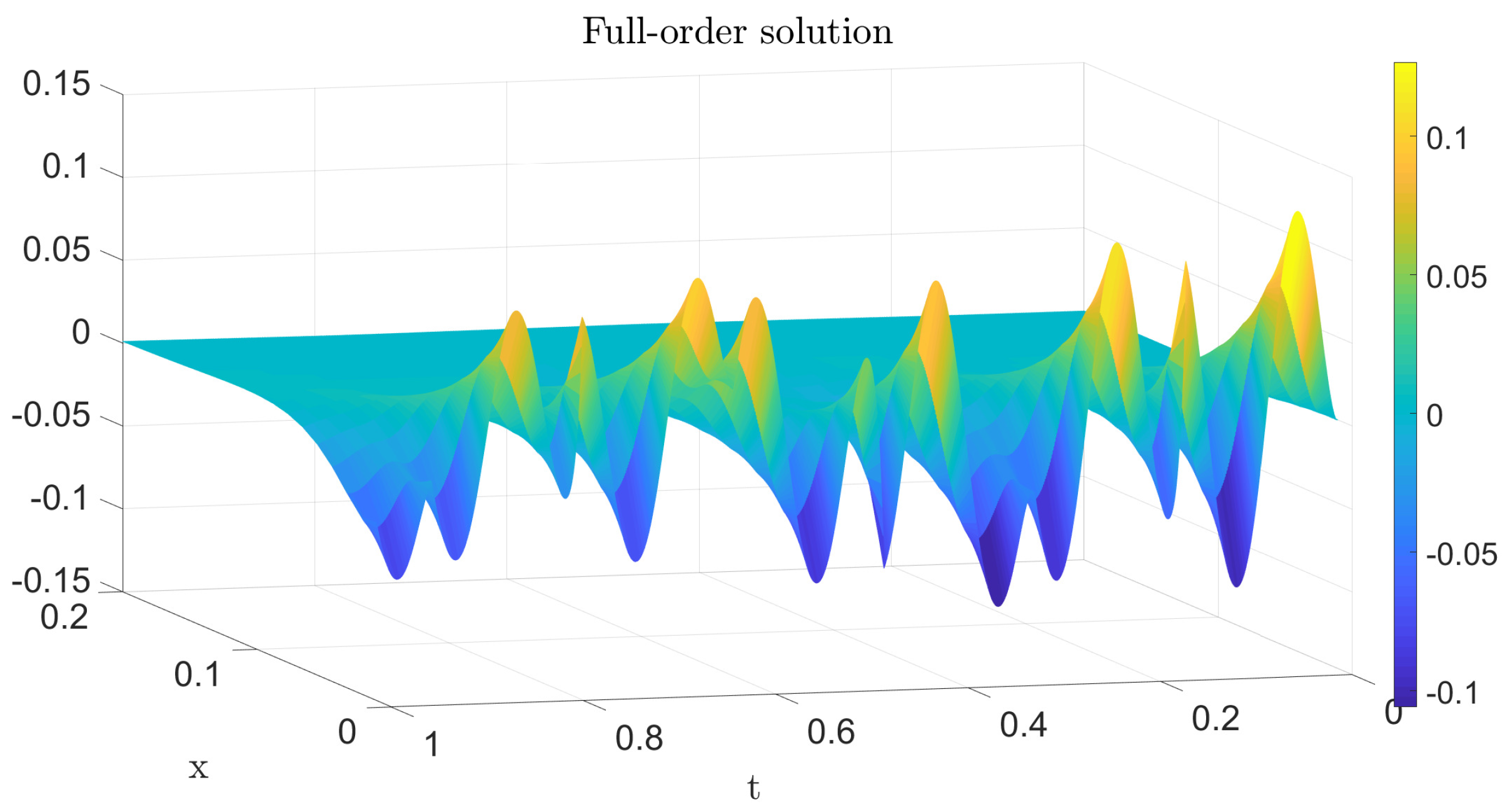
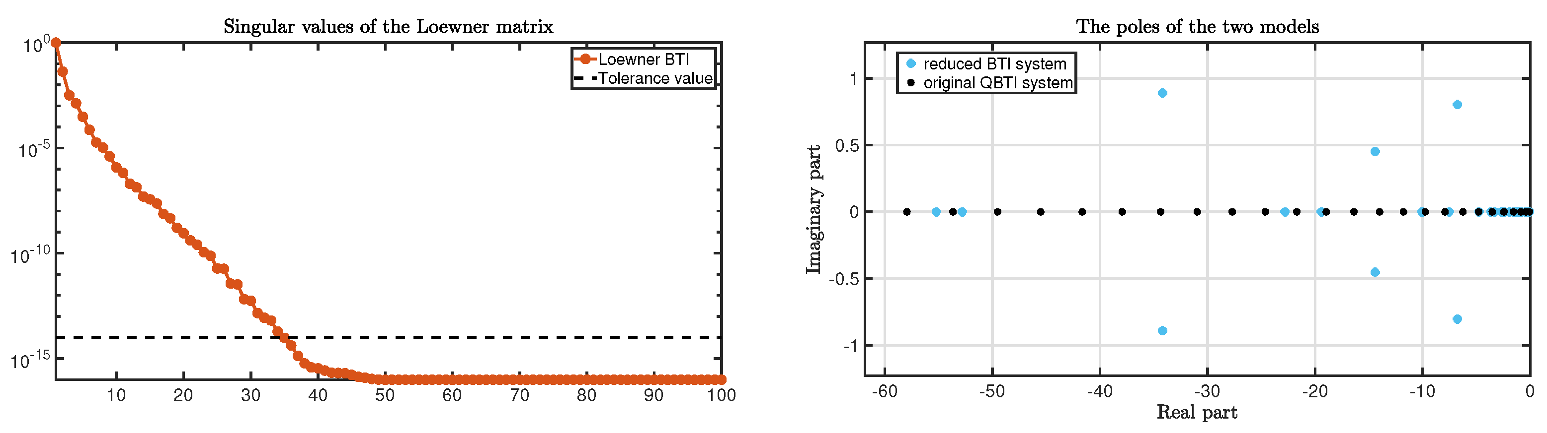
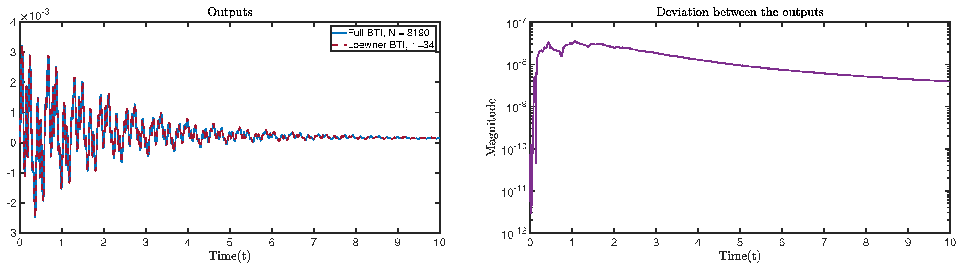
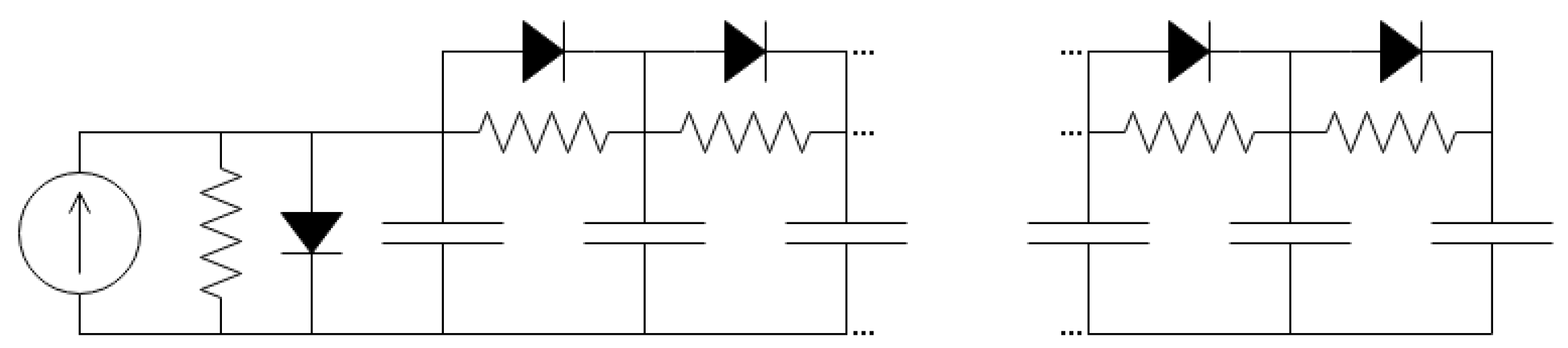
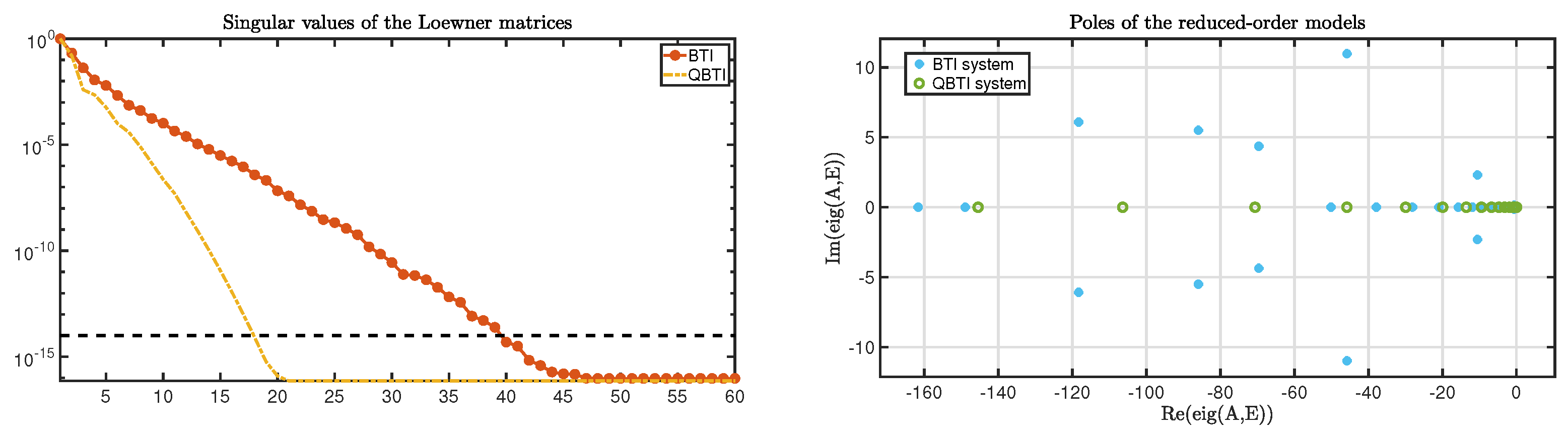
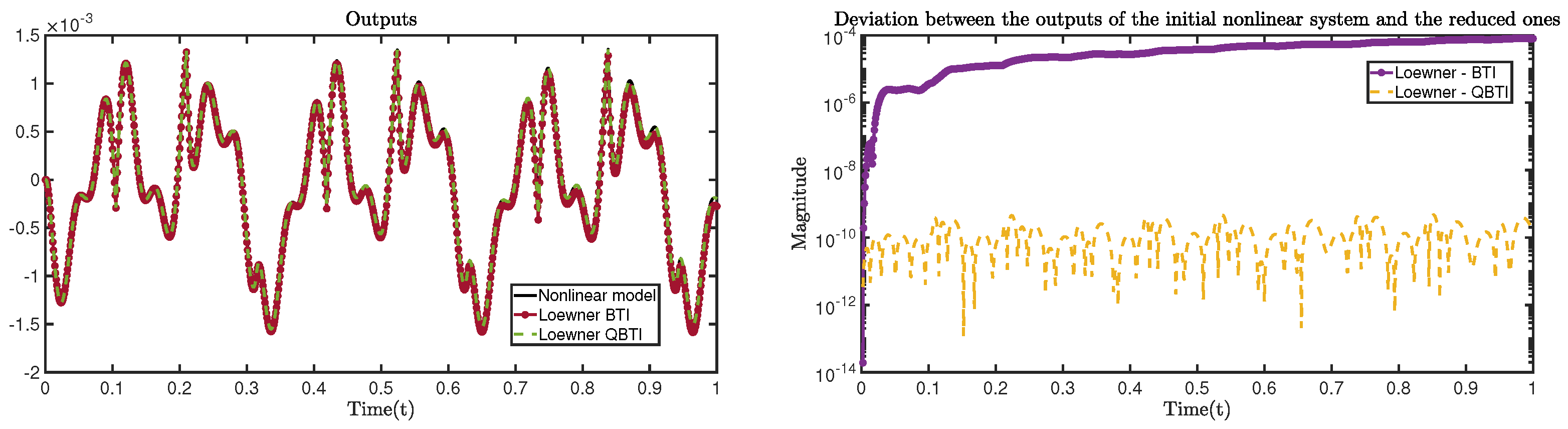
The method used—the Loewner framework—is a data-driven approach that requires samples of generalized transfer functions, which are appropriately defined for both bilinear and quadratic-bilinear systems. We showed explicit relations between these mappings, as well as between the matrices and the poles of the reduced-order models. The theoretical considerations were illustrated by two numerical examples. These included a classical application for computational fluid dynamics (the first), and a nonlinear circuit from the field of electronic engineering. Both numerical test-cases demonstrated connections between the two types of reformulations as indicated by the theory and technical results.

Finally, it was shown that formulating general nonlinear systems as QBTI systems is indeed the approach to be preferred (for applying MOR methods, such as the LF). However, using the reformulation as BTI systems also has its advantages: the simpler structure allows many connections to classical LTI systems theory.

Future research endeavors may potentially include studying the connections between the original QBTI and the BTI lifted model (by Carleman’s approach) in the time domain (by explicitly comparing the Markov parameters of both models), analyzing lifting techniques for recasting nonlinear systems with polynomial nonlinearities as QBTIs, and imposing stability preservation for the reduced-order models.

References

1. Antoulas, A.C. Approximation of Large-Scale Dynamical Systems; SIAM: Philadelphia, PA, USA, 2005. [Google Scholar]
2. Benner, P.; Ohlberger, M.; Cohen, A.; Willcox, K. Model Reduction and Approximation; Society for Industrial and Applied Mathematics: Philadelphia, PA, USA, 2017. [Google Scholar]
3. Antoulas, A.C.; Beattie, C.A.; Gugercin, S. Interpolatory Methods for Model Reduction; SIAM: Philadelphia, PA, USA, 2020. [Google Scholar]
4. Baur, U.; Benner, P.; Feng, L. Model order reduction for linear and nonlinear systems: A system-theoretic perspective. Arch. Comput. Methods Eng. 2014, 21, 331–358. [Google Scholar] [CrossRef]
5. Benner, P.; Breiten, T. Two-sided projection methods for nonlinear model order reduction. SIAM J. Sci. Comput. 2015, 37, B239–B260. [Google Scholar] [CrossRef]
6. Ahmad, M.I.; Benner, P.; Jaimoukha, I. Krylov Subspace Projection Methods for Model Reduction of Quadratic-Bilinear Systems. IET Control Theory Appl. 2016, 10, 2010–2018. [Google Scholar] [CrossRef] [Green Version]
7. Benner, P.; Goyal, P. Balanced Truncation Model Order Reduction for Quadratic-Bilinear Control Systems. arXiv 2017, arXiv:1705.00160. [Google Scholar]
8. Benner, P.; Goyal, P.; Gugercin, S. 2-Quasi-Optimal Model Order Reduction for Quadratic-Bilinear Control Systems. SIAM J. Matrix Anal. Appl. 2018, 39, 983–1032. [Google Scholar] [CrossRef] [Green Version]
9. Ruberti, A.; Isidori, A.; D’Alessandro, P. Theory of Bilinear Dynamical Systems; Springer: Berlin/Heidelberg, Germany, 1972. [Google Scholar]
10. Freund, R. Krylov-subspace methods for reduced-order modeling in circuit simulation. J. Comput. Appl. Math. 2000, 123, 395–421. [Google Scholar] [CrossRef] [Green Version]
11. Zhang, L.; Lam, J. On 2 model reduction of bilinear systems. Automatica 2002, 38, 205–216. [Google Scholar] [CrossRef]
12. Phillips, J.R. Projection-Based Approaches for Model Reduction of Weakly Nonlinear, Time-Varying Systems. IEEE Trans. Comput.-Aided Des. Integr. Circuits 2003, 22, 171–187. [Google Scholar] [CrossRef] [Green Version]
13. Bai, Z.; Skoogh, D. A projection method for model reduction of bilinear dynamical systems. Linear Algebra Appl. 2006, 415, 406–425. [Google Scholar] [CrossRef] [Green Version]
14. Condon, M.; Ivanov, R. Krylov subspaces from bilinear representations of nonlinear systems. COMPEL-Int. J. Comp. Math. Electr. Electron. Eng. 2007, 26, 399–406. [Google Scholar] [CrossRef] [Green Version]
15. Breiten, T.; Damm, T. Krylov subspace methods for model order reduction of bilinear control systems. Syst. Control Lett. 2010, 59, 443–450. [Google Scholar] [CrossRef]
16. Benner, P.; Damm, T. Lyapunov equations, energy functionals, and model order reduction of bilinear and stochastic systems. SIAM J. Control Optim. 2011, 49, 686–711. [Google Scholar] [CrossRef] [Green Version]
17. Benner, P.; Breiten, T. Interpolation-based H2-model reduction of bilinear control systems. SIAM J. Matrix Anal. Appl. 2012, 33, 859–885. [Google Scholar] [CrossRef] [Green Version]
18. Hartmann, C.; Schäfer-Bung, B.; Thöns-Zueva, A. Balanced averaging of bilinear systems with applications to stochastic control. SIAM J. Matrix Anal. Appl. 2013, 51, 2356–2378. [Google Scholar] [CrossRef] [Green Version]
19. Flagg, G.; Gugercin, S. Multipoint Volterra Series Interpolation and H2 Optimal Model Reduction of Bilinear Systems. SIAM J. Matrix Anal. Appl. 2015, 36, 549–579. [Google Scholar] [CrossRef] [Green Version]
20. Antoulas, A.C.; Gosea, I.V.; Ionita, A.C. Model reduction of bilinear systems in the Loewner framework. SIAM J. Sci. Comput. 2016, 38, B889–B916. [Google Scholar] [CrossRef]
21. Karachalios, D.S.; Gosea, I.V.; Antoulas, A.C. On Bilinear Time-Domain Identification and Reduction in the Loewner Framework. In Model Reduction of Complex Dynamical Systems; International Series of Numerical Mathematics; Birkhäuser: Cham, Switzerland, 2021; Volume 171, pp. 3–30. [Google Scholar] [CrossRef]
22. Peherstorfer, B.; Willcox, K. Data-driven operator inference for nonintrusive projection-based model reduction. Comput. Methods Appl. Mech. Eng. 2016, 306, 196–215. [Google Scholar] [CrossRef] [Green Version]
23. Gosea, I.V.; Antoulas, A.C. Data-driven model order reduction of quadratic-bilinear systems. Numer. Linear Algebra Appl. 2018, 25, e2200. [Google Scholar] [CrossRef] [Green Version]
24. Benner, P.; Goyal, P.; Kramer, B.; Peherstorfer, B.; Willcox, K. Operator Inference for Non-Intrusive Model Reduction of Systems with Non-Polynomial Nonlinear Terms. Comput. Methods Appl. Mech. Eng. 2020, 372, 113433. [Google Scholar] [CrossRef]
25. Qian, E.; Krämer, B.; Peherstorfer, B.; Willcox, K. Lift & Learn: Physics-informed machine learning for large-scale nonlinear dynamical systems. Phys. D Nonlinear Phenom. 2020, 406, 132401. [Google Scholar] [CrossRef] [Green Version]
26. Gosea, I.V.; Karachalios, D.S.; Antoulas, A.C. Learning reduced-order models of quadratic dynamical systems from input–output data. In Proceedings of the 2021 IEEE European Control Conference (ECC), Delft, The Netherlands, 29 June–2 July 2021; pp. 1426–1431. [Google Scholar]
27. Kutz, J.N.; Brunton, S.L.; Brunton, B.W.; Proctor, J.L. Dynamic Mode Decomposition: Data-Driven Modeling of Complex Systems; Society of Industrial and Applied Mathematics: Philadelphia, PA, USA, 2016. [Google Scholar] [CrossRef]
28. Alla, A.; Kutz, J.N. Nonlinear Model Order Reduction via Dynamic Mode Decomposition. SIAM J. Sci. Comput. 2017, 39, B778–B796. [Google Scholar] [CrossRef]
29. Goldschmidt, A.; Kaiser, E.; Dubois, J.L.; Brunton, S.L.; Kutz, J.N. Bilinear dynamic mode decomposition for quantum control. New J. Phys. 2021, 23, 033035. [Google Scholar] [CrossRef]
30. Gosea, I.V.; Pontes Duff, I. Toward fitting structured nonlinear systems by means of dynamic mode decomposition. In Model Reduction of Complex Dynamical Systems; International Series of Numerical Mathematics; Birkhäuser: Cham, Switzerland, 2021; Volume 171, pp. 53–74. [Google Scholar] [CrossRef]
31. Mayo, A.J.; Antoulas, A.C. A framework for the generalized realization problem. Linear Algebra Appl. 2007, 426, 634–662. [Google Scholar] [CrossRef] [Green Version]
32. Carleman, T. Application de la théories des équations intégrales linéaires aux systèmes d’équations différentielles non linéaires. Acta. Math. 1932, 59, 63–87. [Google Scholar] [CrossRef]
33. McCormick, G.P. Computability of global solutions to factorable nonconvex programs: Part I—Convex underestimating problems. Math. Program. 1976, 10, 147–175. [Google Scholar] [CrossRef]
34. Gu, C. A projection-based nonlinear model order reduction approach using quadratic-linear representation of nonlinear systems. IEEE Trans. Comput.-Aided Des. Integr. Circuits Syst. 2011, 30, 1307–1320. [Google Scholar] [CrossRef]
35. Kramer, B.; Willcox, K.E. Nonlinear model order reduction via lifting transformations and proper orthogonal decomposition. AIAA J. 2019, 57, 2297–2307. [Google Scholar] [CrossRef]
36. Gu, C. Model Order Reduction of Nonlinear Dynamical Systems. Ph.D. Thesis, EECS Department, University of California, Berkeley, CA, USA, 2012. [Google Scholar]
37. Gilbert, E. Functional expansions for the response of nonlinear differential systems. IEEE Trans. Autom. Control 1977, 22, 909–921. [Google Scholar] [CrossRef]
38. Rugh, W.J. Nonlinear System Theory—The Volterra/Wiener Approach; The Johns Hopkins University Press: Baltimore, MD, USA, 1981. [Google Scholar]
39. Gosea, I.V. Model Order Reduction of Linear and Nonlinear Systems in the Loewner Framework. Ph.D. Thesis, Department of Electrical Engineering, Jacobs University Bremen, Bremen, Germany, 2017. [Google Scholar]
40. Asif, M.M.A.; Ahmad, M.I.; Benner, P.; Feng, L.; Stykel, T. Implicit Higher-Order Moment Matching Technique for Model Reduction of Quadratic-bilinear Systems. J. Frankl. Inst. 2021, 358, 2015–2038. [Google Scholar] [CrossRef]
41. Chen, Y. Model Reduction for Nonlinear Systems. Master’s Thesis, M.I.T, Boston, MA, USA, 1999. [Google Scholar]
42. Breiten, T. Interpolatory Methods for Model Reduction of Large-Scale Dynamical Systems. Ph.D. Dissertation, Department of Mathematics, Otto-von-Guericke University, Magdeburg, Germany, 2013. [Google Scholar] [CrossRef]
43. Antoulas, A.C.; Lefteriu, S.; Ionita, A.C. A tutorial introduction to the Loewner framework for model reduction. In Model Reduction and Approximation; SIAM: Philadelphia, PA, USA, 2017; Chapter 8; pp. 335–376. [Google Scholar]
44. Karachalios, D.S.; Gosea, I.V.; Antoulas, A.C. The Loewner framework for system identification and reduction. In Model Reduction Handbook: Volume I: System- and Data-Driven Methods and Algorithms; Handbook on Model Reduction; Benner, P., Grivet-Talocia, S., Quarteroni, A., Rozza, G., Schilders, W.H.A., Silveira, L.M., Eds.; De Gruyter: Berlin, Germany, 2020; Volume 1. [Google Scholar]
45. Gosea, I.V.; Poussot-Vassal, C.; Antoulas, A.C. Data-driven modeling and control of large-scale dynamical systems in the Loewner framework: Methodology and applications. In Numerical Control: Part A; Handbook on Numerical Analysis; Zuazua, E., Trelat, E., Eds.; Elsevier: Amsterdam, The Netherlands, 2022. [Google Scholar]
46. Antoulas, A.C.; Gosea, I.V.; Heinkenschloss, M. On the Loewner Framework for Model Reduction of Burgers’ Equation. In Active Flow and Combustion Control; King, R., Ed.; Springer: Cham, Switzerland, 2019; pp. 255–270. [Google Scholar]
47. Burgers, J.M. A mathematical model illustrating the theory of turbulence. In Advances in Applied Mechanics; Elsevier: Amsterdam, The Netherlands, 1948; Volume 1, pp. 171–199. [Google Scholar]
Figure 1. The solution of the original full-order QBTI system.
Applsci 12 02333 g001
Figure 2. The singular value decay of the Loewner matrix + tolerance value (left) and the poles of the original QBTI system and of the reduced-order BTI system (right).
Applsci 12 02333 g002
Figure 3. The output of the original large-scale and of the reduced-order BTI systems (left) and the absolute error, i.e., the magnitude of the deviation (right).
Applsci 12 02333 g003
Figure 4. Schematic of the RC ladder circuit from [41].
Applsci 12 02333 g004
Figure 5. The singular value decay of the Loewner matrices of the BTI and QBTI reduced systems (left) and the poles of the reduced-order BTI and QBTI models (right).
Applsci 12 02333 g005
Figure 6. The output corresponding to the original nonlinear system, and to the Loewner BTI and QBTI systems (left) and the magnitude of the absolute errors between the outputs (right).
Applsci 12 02333 g006
Publisher’s Note: MDPI stays neutral with regard to jurisdictional claims in published maps and institutional affiliations.