Abstract
Power Transfer Efficiency (PTE) and Transferred Power (TP) are two crucial indicators of the wireless power transfer (WPT) system. However, in most compensatory topologies, the ideal coils design parameters of PTE and TP are inconsistent, implying that optimizing for one indicator would make another indicator less effective. As a result, in this article, the Thompson sampling efficient multi-objective optimization (TSEMO) algorithm is used to simultaneously optimize PTE and TP in the S-S compensation topology. Through the co-calculation of MATLAB and COMSOL, the coils can be optimized in the environment of magnetic material (ferrite) and conductive material (aluminum). Coils larger than the underwater vehicle’s size are deleted during the data interaction between MATLAB and COMSOL to guarantee that the optimal PTE and TP can be attained within the constrained area. Due to the open standard external software packages between MATLAB and COMSOL, the entire optimization process may be automated. The results show that for WPT systems with restricted input voltage, such as the battery, this design strategy can achieve better TP at the expense of lower PTE, which is highly beneficial in improving the system’s overall performance.
1. Introduction
Magnetic resonance wireless power transfer (MRWPT) is a technology that realizes electric energy transmission utilizing the invisible space medium (magnetic field), eliminating the weaknesses of traditional wire power transmission. In recent years, the security, flexibility, and adaptability of wireless power transmission have received wide attention in academia and business [1,2,3,4]. Especially in the underwater environment, wireless power transfer (WPT) can effectively avoid short circuits, electric leakage, and other safety hazards caused by metal electrode contact [5]. Therefore, developing the WPT system for the underwater environment is of great significance.
When the WPT system is applied underwater, the outer diameter of the coils is usually limited due to the carrying capacity of underwater vehicles. At the same time, magnetic material (ferrite) and conductive material (aluminum) are positioned around the coils to minimize interference from the WPT system’s alternating electromagnetic field, making the coupling design between coils more sophisticated than in the air [6,7].
Power transfer efficiency (PTE) and transferred power (TP), two crucial indicators of a WPT system, have always focused on research and application. As an essential part of the WPT system, the coupling coils plays an important role in transmission performance. It has been reported that the PTE and TP are related to the mutual coupling of coils [8]. In the design process of the WPT, most of the work is coil design and optimization [9]. In order to improve the performance of the WPT system, researchers have done a lot of work on coil structure and parameter optimization. The authors of [10,11] indicated that when the outer diameter of the coils and the inductance are the same, the coupling area between the planar coils is larger, and the space occupied is smaller. The authors of [12,13] had discussed the influence of coils parameters on PTE and TP of the WPT system. Among them, the number of coil turns has the most significant impact, followed by the coil’s inner diameter and wire diameter. Meanwhile, the optimal coils parameters of PTE and TP are not consistent. The authors of [14,15] analyzed the TP of S-S compensation and concluded that, in order to achieve the maximum TP of the WPT system, the coupling coefficient is not as large as possible. In [16], a step-by-step optimization algorithm was proposed, which considered the frequency separation in S-S compensation and improved the system efficiency while meeting the power requirements. However, the space size of the system is free, so the optimized values in practical applications may not be realized in a limited space. In [17], a multi-parameter optimization method was used to optimize the PTE. First, researchers analyzed the PTE and obtained the coils optimization target, and then the exhaustive search algorithm was used to obtain the optimal design parameters. However, the calculation will be tremendous when the number of optimization parameters is three or more. In [18], aimed at maximizing the ratio of coils mutual inductance and resistance, proposed a genetic algorithm (GA) to optimize coils parameters, which reduced the proportion of coils loss in the WPT system and improved the PTE of the system. In [19], the particle swarm optimization (PSO) algorithm was used to optimize coils design to enhance the PTE of the system. It did not use finite element analysis software; therefore, it is difficult to predict and design the coils with magnetic and conductive material around. In the optimization of the above paper, only one of PTE and TP was concerned, but the coils parameters would affect both at the same time. In order to study the influence of coil parameters on PTE and TP simultaneously, the Thompson sampling efficient multi-objective optimization (TSEMO) algorithm [20] was adopted in this paper to optimize coils design. The TSEMO algorithm is a random meta-heuristic algorithm, which accelerates optimization by constructing a Gaussian process agent model and dramatically reduces the calculation cost. It has been successfully applied to global multi-objective optimization of various problems, such as CFD simulation and chemical process simulation [21,22].
In this article, the planar circular coil is taken as the design object, and the coils are optimized around magnetic material (ferrite) and conductive material (aluminum) with a restricted primary and secondary side space size and a certain load resistance. The WPT system adopts S-S topology. When load resistance is given, the relationships between PTE, TP, and coupler parameters are analyzed to obtain coil design parameters and objectives. Then, the TSEMO algorithm is used to find the corresponding design scheme under the spatial constraints. It is highlighted that the design method can be implemented automatically due to the calculation based on MATLAB and COMSOL Multiphysics 5.6 with MATLAB. In addition, the medium around the coupler is freshwater, and its conductivity is generally 0.5 × 10⁻²–5.0 × 10⁻² S/m.
This paper is organized as follows. Section 2 takes S-S compensation topology as an example, analyzes the influence of system parameters on PTE and TP when the load resistance is constant, then obtains the variables and goals of coils design. In Section 3, COMSOL and MATLAB are used for joint calculation, and TSEMO arithmetic is used to find the optimal coils design scheme that meets design objectives. In Section 4, the coil design scheme is simulated first to verify the correctness of the design process, and then the results of traditional design [12,13], M/R single objective optimization [18], and TSEMO optimization are compared. Finally, the conclusion of this study is given in Section 5.
2. Design Variables and Objectives of Planar Circular Coil
The circuit diagram of the S-S compensation topology for the WPT system is shown in Figure 1. AC power UAC represents the high-frequency voltage after the inverter, LP and LS are the self-inductance of the coils, resonant in series with the compensation capacitors CP and CS. M is the mutual inductance between the two coils, RP and RS are AC resistance of coils, IP and IS are the current of the transmitting loop and the receiving loop, respectively, and RL means the load resistance.
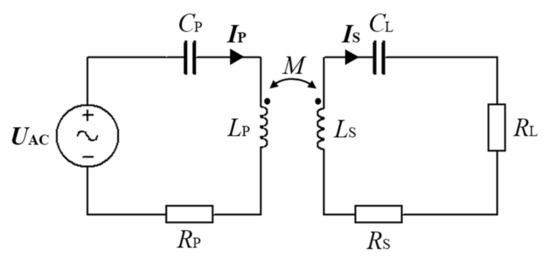
Figure 1.
Circuit diagram of S-S compensation topology.
According to Kirchhoff voltage law (KVL), the equations in Figure 1 is:
Then the expressions of IP, IS, and UL is obtained:
Combining (2), (3), and (4), the PTE and TP can be obtained as
where φuL, φiS, φuAC, and φiP are the phase differences of UL, IS, UAC, and IP, respectively, with respect to the reference sine. For measuring system performance, researchers generally use dimensionless indicators. Therefore, we define the indicators without dimension efficiency η and the voltage modulus gain K when the load resistance is given, the corresponding expressions are as follows:
Then the performance of a WPT system can be described by η and K. According to the expressions when the load resistance RL is determined, the variables affecting η and K includes inverter frequency f, circuit natural angular frequency ω0, mutual inductance M, resistances of coils RP and RS, and self-inductance LP and LS.
Figure 2 shows the coupler structure of the WPT system in this paper. The aluminum plate and ferrite core can shield the electromagnetic field to reduce its influence on the underwater vehicle; simultaneously, the ferrites can increase mutual inductance between two coils. After winding the coil, it is sealed with epoxy resin to avoid displacement and contact with water. Due to the excellent motion performance of the underwater vehicle and the good centering condition of the coupler, the primary and secondary side structures in the design of this paper are the same, namely RP = RS = R and LP = LS = L. Therefore, the design variables are inverter frequency f, circuit natural angular frequency ω0, the mutual inductance of the coils M, coils resistances R, and coils self-inductance L.
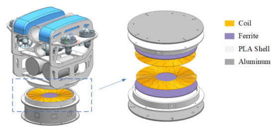
Figure 2.
Coupler structure of the WPT system.
Generally, the mutual inductance and self-inductance of two coils are the inherent parameters of the coupler, only related to the design of the coupler. However, the AC resistance is not only associated with the coupler design, but also affected by the inverter frequency. The inverter frequency of underwater WPT systems is usually between kHz–MHz. When the inner diameter of the copper wire is 2 mm, the coil adopts the traditional design (Coil inner diameter/outer diameter = 0.4, Turn pitch = 3 * Wire inner diameter) [12,13], and the distance between the primary and secondary side is 5 cm (the design distance between the primary side and the secondary side when the underwater vehicle docks with the base station.), the relationship between coil’s self-inductance L, mutual inductance M, and AC resistance R and inverter frequency f is shown in Figure 3.
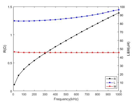
Figure 3.
The relationship between coil’s self-inductance L, mutual inductance M, AC resistance R, and frequency f.
The data show that the mutual inductance and self-inductance do not change much with frequency, while the AC resistance changes greatly. Therefore, we take L = 84.61 μH as an example, when the load resistance RL = 50 Ω, the circuit natural angular frequency ω0 = 2πf0 = 2π·500 kHz, then substitute AC resistance data to solve η and K. The relationship between voltage modulus gain K, inverter frequency f, and mutual inductance M is shown in Figure 4a. Figure 4b illustrates the relationship between efficiency η, inverter frequency f, and mutual inductance M.
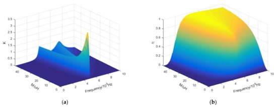
Figure 4.
(a) The relationship between voltage modulus gain K, inverter frequency f, and mutual inductance M; and (b) the relationship between efficiency η, inverter frequency f, and mutual inductance M.
As shown from Figure 4a, the voltage modulus gain K increases first and then sharply decreases with the increase of mutual inductance M and reaches its maximum value at the natural resonant frequency (500 kHz). With the further increase of mutual inductance M, the frequency splitting phenomenon occurs. That is, there are two frequencies to maximize the load voltage. The greater the M, the more fragmentation. Figure 4b illustrates that the efficiency η continues to increase with the increase of mutual inductance M. Meanwhile, when the coupling coefficient is the same, the efficiency at the resonant frequency is the highest.
Obviously, if the coil is optimized for PTE only, the TP will be insufficient when the input voltage is restricted. Similarly, while the TP is ideal, the TPE is only approximately 50%; this lower efficiency is undesirable in engineering applications. To ensure that K and η have good values simultaneously, it is necessary to study the influence of the same frequency and coils parameters for K and η of the WPT system at the same time. Therefore, the partial contour diagram of voltage modulus gain K and system efficiency η is drawn in a coordinate system, as shown in Figure 5.
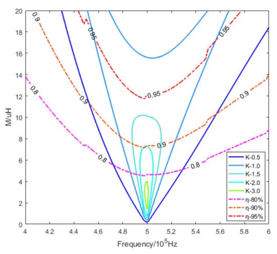
Figure 5.
The partial contour diagram of K and η.
The contour diagram Figure 5 shows that when the mutual inductance of the coils is large, K can be increased at the expense of decreasing η by adjusting the inverter frequency not equal to the natural frequency of the circuit. However, at the same efficiency η, the maximum voltage modulus gain K, meaning the maximum TP, must occur under resonant conditions, where f = f0. Therefore, to ensure that K and η keep good performance simultaneously, the circuit natural resonant frequency f0 should be equal to the inverter frequency f.
According to Equations (2) and (3), the impedance of the secondary side circuit ZS and the impedance reflected from the secondary side to the primary side Zref is:
Then the primary side input impedance ZI is:
When the WPT system works in the resonant state, the current and voltage on the primary side and secondary side are in the same phase, meaning that the imaginary parts of ZI and ZS are zero to maintain the purely resistive. The resonance conditions can be obtained by analyzing Equations (9) and (11):
In the article, LP = LS = L and CP = CS = C, then the inverter frequency f satisfies the condition:
Then the system efficiency η and voltage modulus gain K can be described as follows:
In summary, the design variables only include inverter frequency f, mutual inductance M of the two coils, and coils’ AC resistance R.
During the WPT system charging, the underwater vehicle will be mechanically connected to the base station to prevent the water flow from affecting the system’s stability. At this time, the distance between the two coils remains unchanged, so the coils’ mutual inductance M and coils’ AC resistance R is only related to the coil structure. Figure 6 is the cross-sectional structure model of the planar coil. The coil diameter (2r) usually depends on the current. Then the coil structure can be represented by the inner diameter (Din), the turning pitch (p), and the number of turns (N). Constrained by the mechanical structure in Figure 2, the coils’ maximum outer diameter (Dout) is 300 mm. If the outside diameter of the coils is greater than 300 mm, remove it from the coils group in the simulation calculation to guarantee that the optimal parameters may be reached within a restricted size.
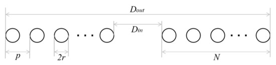
Figure 6.
The cross-sectional structure model of the planar coil.
To summarize, the design objectives for the WPT system are K and η, and corresponding design variables are the inverter frequency f, the inner diameter of coils Din, the turn pitch p, and the number of turns N. By combining the actual conditions, some of the variables’ ranges are removed. The final design variables and ranges are presented in Table 1 below.

Table 1.
The final design variables and ranges.
3. Parameters Optimization Design Based on TSEMO Algorithm
In the last section, we take the S-S topology as an example to determine the PTE and TP of the WPT system to obtain the normalized design objectives K and η. Next, we investigate the influence of various system parameters on K and η, and merge and delete some parameters to obtain the final design variables and their ranges. Obviously, it is time-consuming to calculate all the variable design combinations. The intelligent optimization algorithm can solve this problem well. It can explore the solution space intelligently and dramatically minimize the calculation times.
Figure 7 shows the flowchart of the Thompson sampling efficient multi-objective optimization (TSEMO) algorithm. TSEMO algorithm is an optimization algorithm based on a proxy model. The proxy model of the Gaussian process is established for the actual problem through the current data set, and the next sampling point is determined. After the next sampling point is calculated, update the proxy model, choose the next point, and enter the next round of optimization until it reaches the maximum number of iterations. The introduction of the proxy model avoids the large number of calculations required for random sampling in the sampling space and accelerates the optimization process very well. The TSEMO algorithm’s process building in MATLAB is based on [23].
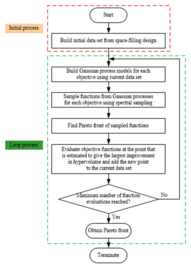
Figure 7.
Algorithm flowchart for TSEMO algorithm.
When taking K and η as optimization objectives, the optimal solution of the S-S coupling mechanism is no longer unique. It will exist in the form of a solution set. The optimal data solution set is called the Pareto front, also called the non-inferior solution set. The parameter value in the Pareto front maximizes one object while maintaining the maximum possible value of other conflicting objects. Solutions suitable to enter the Pareto front are picked by the criteria named Pareto dominance. Pareto dominance can be explained by considering that x1 and x2 both represent arbitrary solutions. For a minimization problem, Pareto dominance states that x1 dominates x2 if their objective function satisfies the following:
where fi represents the value of the ith objective function, namely, x2’s all objective function values are not better than x1’s objective function values, and at least one objective function value of x2 is worse than x1’s. Thus, Pareto advantage is essentially comparing solutions and deciding which solution is non-advantageous. The non-dominant solution is then added to the Pareto front. After obtaining Pareto front data, the conflicts between multiple design objectives can be well weighed by using Pareto front visualization. Then the optimal solution and corresponding design parameters can be obtained.
When the coils are around the environment of magnetic material and conductive material, it is difficult to use the empirical formula to calculate the accurate coils inductance, mutual inductance, and AC resistance. Researchers typically estimate those data in the finite element analysis software after building a simplified model. In COMSOL, the physical field of the model is the magnetic field, and a 2-dimensional axisymmetric model is adopted, so the coupler is usually half-drawn, and the distance between couplers is fixed at 5 cm. The material data is given according to the actual model.
In order to ensure the automatic execution of the optimization process, after building the TSEMO algorithm framework in MATLAB, COMSOL software is used to create the solution model of the coils coupling and then saved it as a script file in MATLAB. In COMSOL Multiphysics 5.6 with MATLAB, you can run the COMSOL solver model as a single function script from within MATLAB. This method enables MATLAB to transfer the coils information generated by input variables to COMSOL script files in the form of TXT files and then receive the simulation output of the COMSOL solution model. Data transmission between the two is completed by reading and writing Excel files. The optimization process is automated through the standard interface of COMSOL and MATLAB. Figure 8 depicts the specific optimization procedure.
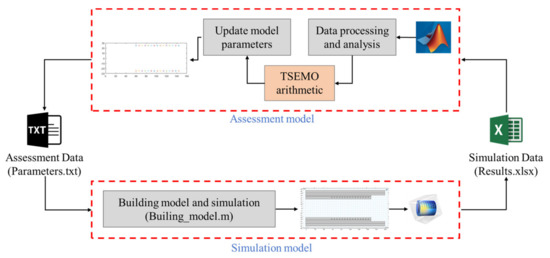
Figure 8.
The structure of automation optimization process.
When RL = 50 Ω, take the initial points as 160, the population number as 25, and the number of iterations as 90 times. In this case, the solution time on the PC is 20 h. The final Pareto front visualization is drawn in Figure 9, where X represents the sampling point in the optimization process of the algorithm, O represents the Pareto front data set and represents the optimal system performance currently found. Obviously, due to the introduction of the Gaussian process proxy model, most algorithm sampling points are near the optimal value, which means even if the optimization time is short, the optimization effect of the optimal value obtained by the optimization process will not be poor.
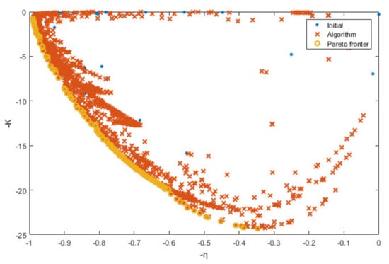
Figure 9.
The visualization of final Pareto front.
The two most important indicators in a WPT system are K and η. Ideally, designers need coils with high K and high η. However, the Pareto front visualization shows that the K and η of S-S compensated WPT system conflict; a specific set of coils can’t achieve the best PTE and TP simultaneously. The main reason for this phenomenon is the frequency separation phenomenon. That is, in the over-coupling state, the system efficiency is very high, but the voltage across the load is much smaller than the under-coupling and critical coupling. When the system input voltage is limited, designers need to choose between PTE and TP according to the actual situation of the system.
The co-simulation of MATLAB and COMSOL makes the optimization program not only get the visualization of efficiency and voltage modulus gain, but also give the date of system frequency and coils position in the coupling structure, ensuring that the optimized value can be easily realized in the limited coupling mechanism.
4. Simulations and Analysis
In Section 3, the multi-objective optimization design of the coupler based on the TSEMO algorithm is presented and optimized at RL = 50 Ω. The Pareto front visualizations of system efficiency η and voltage modules gain K are illustrated, and the frequency and coil variables corresponding to the Pareto front are also obtained. However, in the co-simulation process, there will inevitably be precision loss due to amounts of data storage and rereading, which affects the reliability of the optimization results. Therefore, this section first verifies the reliability of the optimization results, then compares other design schemes to verify the advantages and disadvantages of the optimization results.
4.1. Reliability Analysis of Optimization Results
Under the optimization settings in Section 3, 163 design combinations of the Pareto front are finally obtained. So, this paper only takes representative combinations of the Pareto front for discussion in the analysis stage. Table 2 shows partial Pareto front points and their corresponding frequencies and coils parameters.
Table 2.
Pareto front points and their corresponding parameters.
From Table 2, it is evident that even in the case of random initial data, the increase of coils turns still shows a strong correlation with the improvement of efficiency and the decrease of voltage modulus gain, which is consistent with [12,13]. The main reason is that the mutual inductance M is closely related to the number of turns, and M has a significant influence on η and K. The inner radius of the coils shows a significant fluctuation without apparent regularity. The value of the turn pitch is basically maintained near the given maximum value because the smaller the turn spacing, the bigger the AC resistance of the coils, and the AC resistance is detrimental to both efficiency and voltage modulus gain. Furthermore, it is easier to observe better voltage gain and efficiency at higher frequencies simultaneously.
In order to verify the reliability of the optimization results, the third group of parameters was taken as an example to model and calculate the planar coils coupler values in COMSOL. After that, build the S-S compensation in Multisim to calculate the voltage modulus gain and efficiency. The model and the corresponding results are shown in Figure 10.
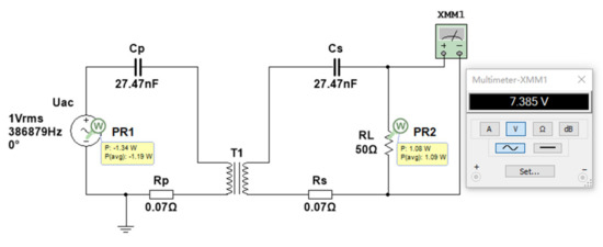
Figure 10.
Multisim simulation model of S-S compensation.
The Multisim simulation data shows that the system’s η = 91.59% and K = 7.39, which is very close to the value of the co-simulation. According to the same simulation method, the simulation values corresponding to the other groups of Pareto front points are obtained as shown in the following Figure 11.
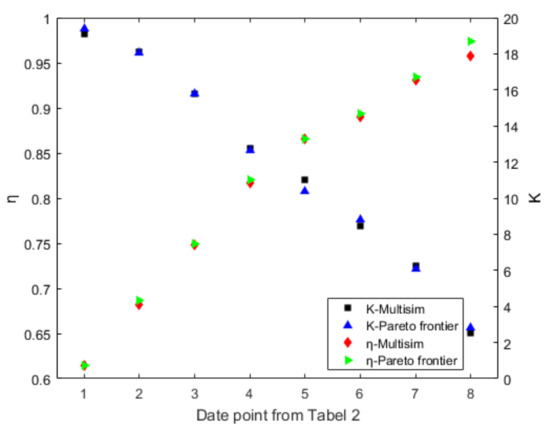
Figure 11.
Efficiency η, voltage modulus gain K of Pareto front and Multisim.
Figure 11 shows that the difference between Pareto front data and Multisim modeling is small, so the results obtained by the optimization process have high reliability and certain application value.
4.2. Comparison with Traditional Design and Single-Objective Optimization
After verifying the reliability of the optimization process, this part compares the design results of traditional design [12,13], single-objective optimization (Maximize M/R to improve efficiency) [18], and multi-objective optimization. Since the optimal solution of multi-objective optimization is the Pareto front data set, it isn’t easy to compare with a single optimization result. At the same time, different design methods will inevitably have different coils parameters; obviously the coils parameters cannot be used as independent variables. After noting that there is an approximately linear relationship between the multi-objective results and the circuit frequency, this paper finally takes the frequency as the abscissa to screen the appropriate Pareto front points and compares the η and K of different designs when RL = 5 Ω, RL = 50 Ω, and RL = 100 Ω, respectively.
Figure 12 illustrates that while the load is the same, both traditional and single-objective optimization designs maintain a high degree of system efficiency over the frequency range. The main reason is that both take a sizeable mutual inductance M as the design indicator, so the system will eventually work in the over-coupling state. In this situation, the system’s PTE can be guaranteed, but it will inevitably lead to lower system PT. However, multi-objective optimization can balance this problem nicely. Taking RL = 50 Ω as an example, the traditional design’s maximum efficiency and voltage gain in the given frequency band are 98.10% and 0.86. The efficiency and voltage modulus gain for multi-objective optimization are 95.24% and 5.01 at 483,279 Hz. The system achieves 5.83 times voltage gain at the cost of 2.87% efficiency, which means the TP will increase 34 times, and the final system PTE of 95.24% is still within the acceptable engineering range. Compared with the M/R single-objective optimization of PTE design, the multi-objective optimization can improve the TP 12.8 times under the cost of 3% TPE, which makes sense for input voltage-constrained systems.
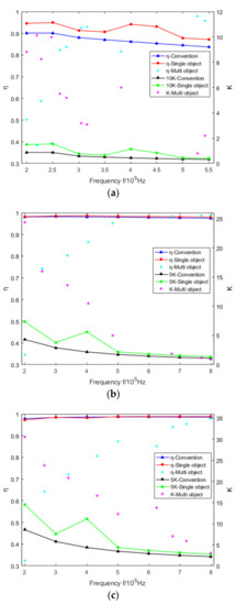
Figure 12.
Efficiency η, voltage modulus gain K of traditional design, single-objective optimization, and multi-objective optimization. (a) The load resistance RL = 5 Ω. (b) The load resistance RL = 50 Ω. (c) The load resistance RL = 100 Ω.
It can also be obtained from Figure 12 that the smaller the load resistance RL, the better the multi-objective optimization effect. The main reason is that the load resistance doesn’t connect with the optimization target in traditional design and single-objective optimization. When the load resistance is low, the secondary side’s voltage sharing capability is decreased, and the power consumed on the coils is increased, so the PTE and TP of the system reduce at the same time. Meanwhile, it is obvious from Figure 12a–c that the two optimization results are better than the traditional design at some point. As a result, it’s critical to optimize parameters in the design stage based on the desired design objectives.
Figure 13 depicts the Pareto front curves optimized under different load resistance. Obviously, the larger the load, the more likely it is to obtain and maintain the ideal PTE and TP simultaneously. As a result, a careful selection of load resistance during the system design stage can help to improve system performance.
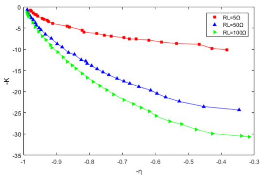
Figure 13.
Pareto front curves under different load resistance.
4.3. Optimization Consistency Analysis between Optimization Results and Experiments
In order to verify the aforementioned analysis results, we set up the experiment prototype illustrated in Figure 14, and pick a set of coil design parameters under traditional design, M/R single-objective optimization, and multi-objective optimization for experiments when RL = 53.2 Ω.
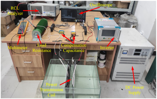
Figure 14.
The experiment setup.
When the power on the load resistor RL is about 200 W, the power transmission efficiency η for traditional design, M/R single-objective optimization, and multi-objective optimization are 93.2%, 93.5%, and 86.3%, respectively, and the input voltage of the power supply is 131 V, 112 V, and 35 V, which means the voltage modulus gain K are 0.82, 0.94, and 3.45, respectively. In the experiment, the equivalent resistance of the capacitor and the resistance of the connecting wire have an effect on the power transmission efficiency η and the voltage modulus gain K. The multi-objective optimization’s coil resistance is smallest, meaning it is the most affected. In addition, coils in the experiment are not totally symmetrical, and the load resistance has a little inductance; it’s hard to make the power transmission coils in resonance condition at the same time, which will reduce efficiency. Further, some iron clips that will increase the magnetic field are around coils, and there are measurement errors. Due to these factors, the phenomenon whereby experimental results are lower than the theoretical experimental results are reasonable and acceptable.
In total, multi-objective optimization of coil parameters can achieve higher voltage gain at the small cost of efficiency, which can guide the design process when the range of input power supply is restricted. The theoretical analysis is confirmed by experimental results.
5. Conclusions
This article takes S-S compensation topology as an example and analyzes the relationship between power transfer efficiency (PTE), transferred power (TP), and system parameters. The normalized optimization objectives K and η and corresponding design variables are obtained. When the input voltage range is restricted, in order to ensure that K and η have ideal values at the same time, the TESOM algorithm is used to optimize both of them at the same time. Finally, the Pareto front visualization is shown, which allows designers to easily balance two design goals. COMSOL and MATLAB allow for the automated optimization design of coils in a complicated environment. The coils beyond the size of the underwater vehicle are deleted during the data transmission step of the joint computation to guarantee that the optimal values can be acquired in the restricted area of the underwater vehicle. Experiments show that, compared to traditional design and maximize of M/R to improve efficiency, multi-objective optimization of coil parameters can achieve higher voltage gain at the expense of efficiency, which can guide the design process when the range of input power supply is restricted, such as battery power supply.
Although the compensation topology and coupler structure are chosen throughout the optimization process, these two factors have no bearing on the automated optimization process. The optimization technique in this study may be easily extended to the design of coil couplers with different topology, surroundings and size limitations by deriving alternative compensation topology equations and developing additional coupler models.
Author Contributions
Conceptualization, Y.M.; methodology, Y.M. and Z.M.; software, Y.M.; validation, Y.M.; formal analysis, Y.M. and Z.M. and K.Z.; investigation, Y.M.; resources, Y.M.; data curation, Y.M.; writing—original draft, Y.M.; writing—review and editing, Y.M., Z.M., and K.Z.; visualization, Y.M.; supervision, Z.M. and K.Z.; project administration, Z.M. and K.Z.; funding acquisition, Z.M. and K.Z. All authors have read and agreed to the published version of the manuscript.
Funding
This research was funded by the National Natural Science Foundation of China, grant number 52171338.
Institutional Review Board Statement
Not applicable.
Informed Consent Statement
Not applicable.
Data Availability Statement
Not applicable.
Acknowledgments
Not applicable.
Conflicts of Interest
The authors declare no conflict of interest.
References
- Zhang, Z.; Pang, H.; Georgiadis, A.; Cecati, C. Wireless Power Transfer—An Overview. IEEE Trans. Ind. Electron. 2019, 66, 1044–1058. [Google Scholar] [CrossRef]
- Ramezani, A.; Farhangi, S.; Iman-Eini, H.; Farhangi, B.; Rahimi, R.; Moradi, G.R. Optimized LCC-Series Compensated Resonant Network for Stationary Wireless EV Chargers. IEEE Trans. Ind. Electron. 2019, 66, 2756–2765. [Google Scholar] [CrossRef]
- Jiang, Y.; Wang, L.; Wang, Y.; Liu, J.; Wu, M.; Ning, G. Analysis, Design, and Implementation of WPT System for EV’s Battery Charging Based on Optimal Operation Frequency Range. IEEE Trans. Power Electron. 2019, 34, 6890–6905. [Google Scholar] [CrossRef]
- Lin, W.; Ziolkowski, R.W.; Huang, J. Electrically Small, Low-Profile, Highly Efficient, Huygens Dipole Rectennas for Wirelessly Powering Internet-of-Things Devices. IEEE Trans. Antenn. Propag. 2019, 67, 3670–3679. [Google Scholar] [CrossRef]
- Anyapo, C.; Intani, P. Wireless Power Transfer for Autonomous Underwater Vehicle. In Proceedings of the 2020 IEEE PELS Workshop on Emerging Technologies: Wireless Power Transfer (WoW), Seoul, Korea, 15–19 November 2020; pp. 246–249. [Google Scholar] [CrossRef]
- Budhia, M.; Covic, G.A.; Boys, J.T. Design and Optimization of Circular Magnetic Structures for Lumped Inductive Power Transfer Systems. IEEE Trans. Power Electron. 2011, 26, 3096–3108. [Google Scholar] [CrossRef]
- Lee, I.; Kim, N.; Cho, I.; Hong, I. Design of a Patterned Soft Magnetic Structure to Reduce Magnetic Flux Leakage of Magnetic Induction Wireless Power Transfer Systems. IEEE Trans. Electromagn. Compat. 2017, 59, 1856–1863. [Google Scholar] [CrossRef]
- Kiani, M.; Jow, U.; Ghovanloo, M. Design and Optimization of a 3-Coil Inductive Link for Efficient Wireless Power Transmission. IEEE Trans. Biomed. Circuits Syst. 2011, 5, 579–591. [Google Scholar] [CrossRef] [PubMed] [Green Version]
- Kim, J.; Kim, J.; Kong, S.; Kim, H.; Suh, I.; Suh, N.P.; Cho, D.; Kim, J.; Ahn, S. Coil Design and Shielding Methods for a Magnetic Resonant Wireless Power Transfer System. Proc. IEEE 2013, 101, 1332–1342. [Google Scholar] [CrossRef]
- Laskovski, A.N.; Yuce, M.R.; Dissanayake, T. Stacked Spirals for Biosensor Telemetry. IEEE Sens. J. 2011, 11, 1484–1490. [Google Scholar] [CrossRef]
- Zierhofer, C.M.; Hochmair, E.S. Geometric approach for coupling enhancement of magnetically coupled coils. IEEE Trans. Biomed. Eng. 1996, 43, 708–714. [Google Scholar] [CrossRef] [PubMed]
- Waters, B.H.; Mahoney, B.J.; Lee, G.; Smith, J.R. Optimal coil size ratios for wireless power transfer applications. In Proceedings of the 2014 IEEE International Symposium on Circuits and Systems (ISCAS), Melbourne, Australia, 1–5 June 2014; pp. 2045–2048. [Google Scholar] [CrossRef]
- Jiang, D.; Yang, Y.; Liu, F.; Ruan, X.; Chen, X. Optimization of coils for magnetically coupled resonant wireless power transfer system based on maximum output power. In Proceedings of the 2016 IEEE Applied Power Electronics Conference and Exposition (APEC), Long Beach, CA, USA, 20–24 March 2016; pp. 1788–1794. [Google Scholar] [CrossRef]
- Li, H.L.; Hu, A.P.; Covic, G.A.; Tang, C.S. Optimal coupling condition of IPT system for achieving maximum power transfer. Electron. Lett. 2009, 45, 76–77. [Google Scholar] [CrossRef]
- Wang, C.S.; Covic, G.A.; Stielau, O.H. Power Transfer Capability and Bifurcation Phenomena of Loosely Coupled Inductive Power Transfer Systems. IEEE Trans. Ind. Electron. 2004, 51, 148–157. [Google Scholar] [CrossRef]
- Dehghanian, M.; Namadmalan, A.; Saradarzadeh, M. Optimum design for Series-Series compensated Inductive Power Transfer systems. In Proceedings of the 2017 8th Power Electronics, Drive Systems & Technologies Conference (PEDSTC), Mashhad, Iran, 14–16 February 2017; pp. 365–370. [Google Scholar] [CrossRef]
- Sampath, J.; Alphones, A.; Shimasaki, H. Coil design guidelines for high efficiency of wireless power transfer (WPT). In Proceedings of the 2016 IEEE Region 10 Conference (TENCON), Singapore, 22–25 November 2016; pp. 726–729. [Google Scholar] [CrossRef]
- Xiao, J.; Xiao, L.K.; Wu, N.; Zhu, W.J.; Feng, Y. Novel Planar Circle Coil Design for Magnetic Coupled Wireless Power Transfer System. Electr. Energy Manag. Technol. 2019, 17, 42. [Google Scholar]
- Wei, G.; Jin, X.; Wang, C.; Feng, J.; Zhu, C.; Matveevich, M.I. An Automatic Coil Design Method With Modified AC Resistance Evaluation for Achieving Maximum Coil–Coil Efficiency in WPT Systems. IEEE Trans. Power Electron. 2020, 35, 6114–6126. [Google Scholar] [CrossRef]
- Bradford, E.; Schweidtmann, A.M.; Lapkin, A. Efficient multiobjective optimization employing Gaussian processes, spectral sampling and a genetic algorithm. J. Glob. Optim. 2018, 71, 407–438. [Google Scholar] [CrossRef] [Green Version]
- Helmdach, D.; Yaseneva, P.; Heer, P.K.; Schweidtmann, A.M.; Lapkin, A.A. A Multiobjective Optimization Including Results of Life Cycle Assessment in Developing Biorenewables-Based Processes. ChemSusChem 2017, 10, 3632. [Google Scholar] [CrossRef] [PubMed]
- Yanru, H.; Baowei, S.; Huachao, D. Multi-objective optimization design for the multi-bubble pressure cabin in BWB underwater glider. Int. J. Nav. Archit. Ocean Eng. 2018, 10, 439–449. [Google Scholar] [CrossRef]
- Artur, S. Multi-Objective Optimization Algorithm for Expensive-to-Evaluate Function. GitHub. Available online: https://github.com/Eric-Bradford/TS-EMO (accessed on 5 November 2021).
Publisher’s Note: MDPI stays neutral with regard to jurisdictional claims in published maps and institutional affiliations. |
© 2022 by the authors. Licensee MDPI, Basel, Switzerland. This article is an open access article distributed under the terms and conditions of the Creative Commons Attribution (CC BY) license (https://creativecommons.org/licenses/by/4.0/).