On the Optimal Design of Steel Shells with Technological Constraints

Abstract

This paper is concerned with determining the optimum conditions of steel cylindrical shells with technological limitations and one behavioral constraint, related to a specific constitutive law for limiting load-carrying capacity. The optimum structural design in the plastic range of circular cylindrical full shells composed of rings of variable thickness is given. A numerical procedure for determining the optimal dimensions of shell rings is given. A shell collapse mechanism is assumed in the kinematic part, which satisfies requirements. Within the optimum conditions, the power of the dissipation energy of rings assuming the hexagon Hodge condition of plasticity are derived. A series of numerical solutions and results of optimal structural designs for a shell that is simply supported at the ends are presented. In one example of optimally calculated shells, the length X₁ of one ring was varied.

1. Introduction

We consider the structural optimal design of a circular cylindrical shell composed of rings. The objective function is cost C of the shell. Satisfying the condition of the minimal cost C, we obtained the minimal volume of the shell. First, we used the general structure optimization theory in the plastic region, first developed by Drucker, Shield, Prager, Save, and others. In this procedure, we determined the absolute minimum cost of an optimum structural design for real circular cylindrical shell structures. The problems highlighted here include limited analysis, optimum conditions of shells for yield condition, and optimum plastic dimensioning of the steel shells with rings of different thicknesses. When we consider the shell in the plastic area, in comparison to the elastic, there is a significant plastic reserve in the material and we are able to determine the value of the ultimate load when a fracture occurs. By optimizing for the same load, we obtained the minimum material, i.e., minimum shell volume.

Deriving the optimum conditions and the optimal dimensioning of the shells, we were able to minimize the power of dissipation energy under the given limit load that leads to plastic collapse.

For technological reasons, we treated the shell with rings because this makes it easier to perform in practice. We determined the optimal conditions with technological constraints. Thus, the thickness $e_i$ of the ring must be within the limits: minimum $e_{i,\inf }\le e_i$, and maximum $e_{i,\sup }\ge e_i$. In this way, we ensure that, in cross-sections, the shell thickness is large enough to satisfy the influence of shear forces. In certain cases, technological limitations can be introduced due to functionality reasons.

Often, designs that are difficult to execute (thickness may turn out to be exceedingly small), or that violate basic assumptions of the theory of shell optimization (far too great a thickness in comparison to diameter), are avoided.

In the optimum plastic design of structures, the theory is much more advanced than the experiments. In particular, this discrepancy refers to the optimal dimensioning of the shells, where new publications have been published [1,2]. Among others, the experiments of Kouam [3] in Guerlement’s laboratory demonstrated the application of limit analysis theory for the optimization of cylindrical shells.

Engineers have a specific role in that they must satisfy all requirements regarding determining and dimensioning in industry and practice [4,5]. Structural optimum design requires an individualized approach, as no general method for solving these problems has been established. When optimizing a structure i.e., of its material, the principle of minimum potential deformation energy in elastic and minimum power of dissipation energy in plastic region is applied. In more complex cases, both ranges and two kinds of energies are minimized [6,7]. The commercial engineering optimization software packages based on the finite element method are currently used by researchers to solve standard and non-standard engineering problems. Recently, a large number of papers related to shell problems, as well as optimization in various fields, have emerged from both theoretical and numerical and technological and practical aspects [8].

Optimization is especially important when there is a need for a large series of the same elements or structures. Additionally, in certain cases, the requirements are that the weight of the construction must be as small as possible, i.e., optimal, for example, in the case of aircrafts. An increasing number of papers concerning this have appeared in the last decade. A small number of papers, due to the complexity of this problem, do not have analytical solutions, but most often apply the finite element method [9,10]. New directions for research have evolved in this field. In the paper [11], a purely numerical approach based on optimized numerical integration for probabilistic modeling of a fatigue crack progression is used. More complex shell structures are solved due to different types of loads related to the problem of stability-buckling and dynamics [12,13]. In [14], a non-linear formulation is derived for the assessment of a load of cylindrical shells subjected to pressure, which accounts for the onset of plasticity, including the effect of geometrical imperfections. Shell structures are very important in civil engineering, mechanical engineering, aerospace, and other disciplines. In paper [15], in the frame of the structural analysis of shell structures, the elastic region was extended to the plastic region and the formulation carried out in this paper includes large strain plastic deformation. The shells are represented in the petrochemical industry as shell-and-tube heat exchangers. The study in [16] focuses on the calculations for obtaining the fields of equivalent stresses and plastic deformations.

An optimal design of shells in the elastic region of various constraints has been implemented in [17]. The weight efficiency for various types of shells reinforcements was studied.

For practical, very complex problems concerning the interaction of two shells, as is the case in [18], an optimization method is presented, which combines a finite element method analysis and an optimization algorithm where load path optimization is performed to minimize rod force.

The method of genetic algorithms has been successfully applied to the problem of optimal dimensioning of rotationally symmetric shells [19]. Combining mathematical programming, the finite element method, and the limit analysis of shells, the limit load was calculated and the genetic algorithm led to research concerning the optimal shell using a search heuristic method.

To optimize steel shells in the plastic area considered in this paper, it is necessary to determine the limit analysis of the shell.

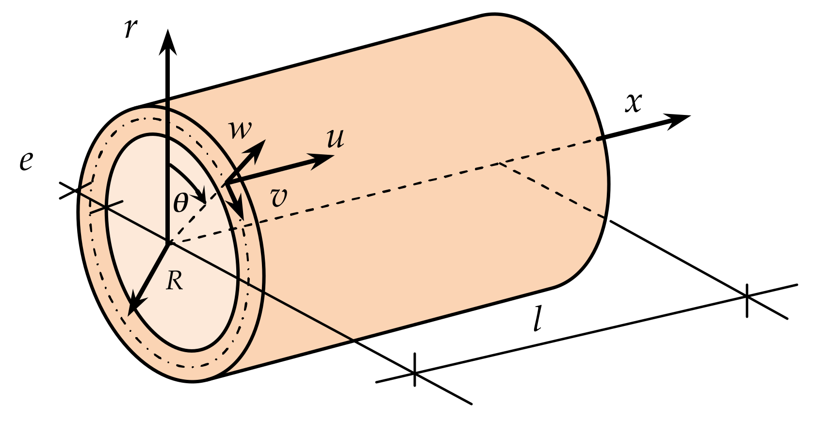
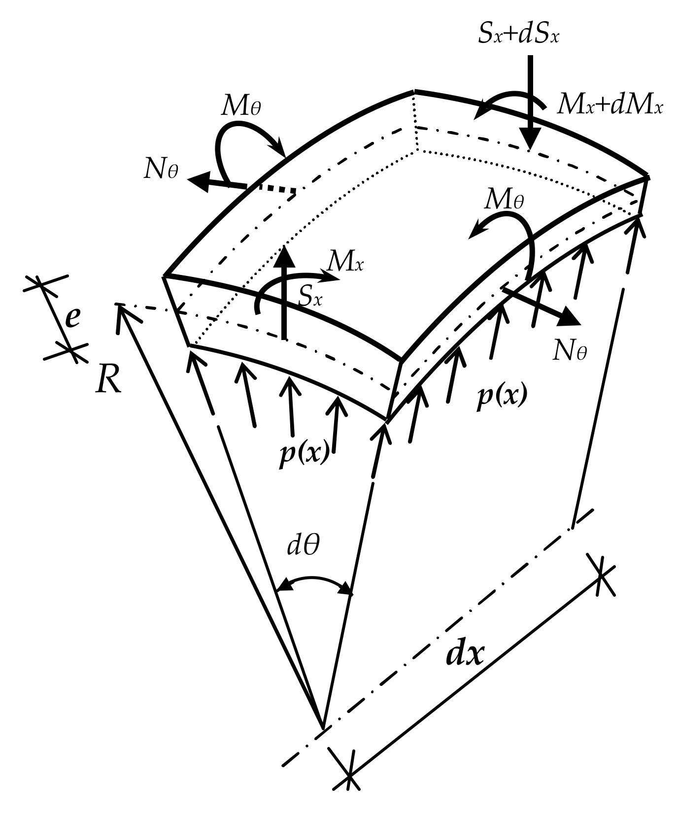
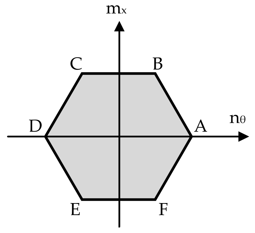
2. Basic Equations for the Limit Analysis of Shells

We observe a simple case of a circular cylindrical shell subjected to pressure p(x) in the outward radial direction. A homogeneous and orthotropic material with rigid, perfectly plastic behavior is considered. The cylindrical coordinate system (r, θ, x) is chosen with the axis x, along with the symmetry. All functions depend on x only. The only displacement of the median surface of the shell is in the radial direction. For the assumption that the elements normal to the median surface are straight and normal after deformation, see Figure 1.

The power of dissipation energy $\mathcal{D}$ across a shell element is given by

$$\mathcal{D}={\displaystyle \underset{-e/2}{\overset{+e/2}{\int }}\left({\sigma }_x{\dot{\epsilon }}_x+{\sigma }_0{\dot{\epsilon }}_{\theta }\right)dz},$$

(1)

${\dot{\epsilon }}_{\theta }$ and ${\dot{\epsilon }}_x$ are the strain rates of unit circular and axial lengths. It follows as

$$\mathcal{D}=\frac{d^2\dot{w}}{d{x}^2}{M}_x+\frac{\dot{w}}{R}{N}_{\theta }$$

(2)

where the stress resultants M_x and N_θ are introduced (See Figure 2). Introducing the dimensionless values m_x and n_{θ, i.e.},

$$m_x=\frac{M_x}{M_{px}}, n_{\theta }=\frac{N_{\theta }}{N_{p\theta }}$$

(3)

where

$$M_{px}=\frac{{\sigma }_0{e}^2}{4}, N_{p\theta }={\sigma }_{0}e.$$

(4)

The dissipation $\mathcal{D}$ from (1) is given

$$\mathcal{D}={\sigma }_{0}e\left({\dot{k}}_x{m}_x+{\dot{\lambda }}_{\theta }{n}_{\theta }\right).$$

(5)

The strain rates ${\dot{k}}_x$ and $\dot{\lambda }$ corresponding to the generalized stresses $m_x$ and $n_{\theta }$ respectively are the generalized strain rates

$${\dot{k}}_x=\frac{e}{4}\frac{d^2\dot{w}}{d{x}^2}, {\dot{\lambda }}_{\theta }=\frac{\dot{w}}{R}$$

(6)

where $\dot{w}$ is the displacement rate of the median surface of the shell.

The equilibrium of the shell differential element leads to the differential equation

$$\frac{d^2{M}_x}{d{x}^2}+\frac{N_{\theta }}{R}-p\left(x\right)=0.$$

(7)

By denoting M_x and N_θ from (3), Equation (7) reads

$$\frac{d^2{m}_x}{d{x}^2}+2{\omega }^2\left(n_{\theta }-\overline{p}\right)=0,$$

(8)

where

$${\omega }^2=\frac{2}{eR}, \overline{p}=p\frac{R}{{\sigma }_{0}e}.$$

(9)

Hodge’s yield condition. The yield condition shows the points of the structure where stresses M_x and N_θ are in a state of plasticity. Unlike the previous ones, the stresses M_θ and T_x do not appear in the dissipation and represent a reaction correlating to the work by Prager [7]. Starting from Tresca’s material, we obtained a nonlinear interaction curve. On the suggestion of Drucker, the linear approximation was made [20]. Using dimensionless variables $n_{\theta }$$m_x$, the result was Hodge’s hexagon (see Figure 3).

For a shell element in a limited state, the stresses are represented by a point on Hodge’s hexagon. The sides of the hexagon provide the relationship variables m and n given in Hodge’s Table 11-1 in [21] (p. 277). For each side of the hexagon, we find $\dot{w}$ with (6), $\dot{w}$ is a continuous function.

3. Conditions of Minimum Cost Plastic Design of Full Steel Cylindrical Shells

3.1. Hypothesis

Let there be the cylindrical shell (Figure 4) whose middle surface area and boundary conditions are known. The material which constitutes a rigid plastic shell has the yield stress σ_o. Shell layout is divided into n rings bound by the known abscissas. The technological constraints are as follows: $e_{i,inf}\le e_i\le e_{i,sup}$. The problem can be expressed in the following way:

The total cost C of the shell is given as

$$C={\displaystyle \sum _{i=1}^n{A}_i{c}_i}\hspace{0.17em},$$

(10)

where $A_i=2\pi R{l}_i$, i = 1, …, n and c_i is specific cost, i.e., cost per unit of middle surface area of the ring number i. We assume that the specific cost is a function of the thickness of the ring, e_i. The problem of the optimal plastic design of the shell is set as follows: find the set of values e_i (i = 1, …, n) such that the shell is exactly on the verge of collapse under load p(x), to meet technological constraints and the total cost C of the shell (the objective function) be minimal.

We assume that the specific cost c_i is the function of thickness e_i.

Suppose without loss of generality, an external, uniformly distributed load p(x). As is usual for thin shells, volume forces are ignored. The stresses in the shell due to volume forces are many times lower than the stresses caused by the limit load where the yield stress of steel is ${\sigma }_0=235 \mathrm{M}\mathrm{P}\mathrm{a}$.

3.2. Sufficient Optimality Conditions for the Full Shell Case

The structural design is expressed through the shell thicknesses of the rings, e_i. The shell under load p(x) is exactly on the verge of collapse. The collapse mechanism describes a displacement velocity field. Using the combined theorem of the limit analysis, we can write

$${\displaystyle \underset{A}{\int }p(x)}\dot{w}(x)\mathrm{d}A={\displaystyle \sum _{i=1}^n{D}_i}\hspace{0.17em},$$

(11)

Let a neighboring design $e_i^{*}=e_i+\delta e_i$ meet technological constraints so that it can at least sustain a given load. The upper bound theorem of the limit analysis implies

$${\displaystyle \underset{A}{\int }p\left(x\right)}\dot{w}\left(x\right)\mathrm{d}A\le {\displaystyle \sum _{i=1}^n{\mathcal{D}}_{{}_i}^{*}=}{\displaystyle \sum _{i=1}^n{\mathcal{D}}_i+{\displaystyle \sum _{i=1}^n\delta e_i\frac{\partial {\mathcal{D}}_i}{\partial e_i}}}.$$

(12)

The field of displacements rates ${\dot{w}}_x^{\left(i\right)}$ is added to the dimensioning e_i, but is only allowed for dimensioning e_i* and therefore an inequality sign is established. The specific power of dissipation energy ${\mathcal{D}}_i\left[\dot{w}\left(x\right)\right]$ is assumed to be a continuously differentiable function at e_i. Thus, we have

$${\displaystyle \sum _{i=1}^n\delta e_i}\frac{\partial {\mathcal{D}}_i}{\partial e_i}\ge 0$$

(13)

Suppose that the collapse mechanism,$\dot{w}\left(x\right)$, is such that

$$\frac{\partial {\mathcal{D}}_i}{\partial e_i}={\left(\frac{dc}{de}\right)}_{\begin{array}{l}e=e_i\\ c=c_i\end{array}}{A}_i+t_i, i=1, \dots , n,$$

(14)

where t_i, i = 1, …, n, are constants and $A_i$ is the surface of the midline of the ring with thickness e_i. From (13) with (14) we have

$${\displaystyle \sum _{i=1}^n\delta e_i}{\left(\frac{dc}{de}\right)}_{\begin{array}{l}e=e_i\\ c=c_i\end{array}}{A}_i+{\displaystyle \sum _{i=1}^n\delta e_i}{t}_i\ge 0,i=1, \dots , n,$$

(15)

Analyzing the previous relation, we obtain

$$\frac{\partial {\mathcal{D}}_i}{\partial e_i}\le {\left(\frac{dc}{de}\right)}_{\begin{array}{l}e=e_i\\ c=c_i\end{array}}{A}_i, \mathrm{for} e_i=e_{i,inf},$$

(16)

$$\frac{\partial D_i}{\partial e_i}\ge {\left(\frac{dc}{de}\right)}_{e=e_i}{A}_i, \mathrm{for} e_i=e_{i,sup},$$

(17)

$$\frac{\partial D_i}{\partial e_i}={\left(\frac{dc}{de}\right)}_{e=e_i}{A}_i, \mathrm{for} e_{i,inf}<e_i<e_{i,sup}.$$

(18)

For the Inequalities (16) and (17) were $\delta e_i{t}_i\le 0$ and to obtain Equation (18) was $t_i=0$. For the previous analysis, the Inequality (15) can be written in a stronger form

$${\displaystyle \sum _{i=1}^n\delta e_i}{\left(\frac{dc}{de}\right)}_{\begin{array}{l}e=e_i\\ c=c_i\end{array}}{A}_i\ge 0,$$

(19)

which indicates that the design e_i* includes a higher cost than design e_i.

The relationships (16), (17), and (18) represent relative minimum cost.

3.3. Necessary Optimality Conditions for the Full Shell Case

Let e_i be the design that satisfies all the technological constraints, which is exactly on the verge of collapse due to external loads p(x) and gives the minimum total cost C of the shell. Starting with (11) we make a dimensioning change e_i. The corresponding collapse mechanism obtains another strain displacement $\dot{w}$ as well as another limit load p. Thus, Equation (11) becomes

$${\displaystyle \sum _{i=1}^n\left(\frac{\partial {\mathcal{D}}_i}{\partial e_i}\delta e_i+\frac{\partial {\mathcal{D}}_i}{\partial \dot{w}}\delta \dot{w}\right)}={\displaystyle \underset{A}{\int }\left(\frac{\partial \left(p \dot{w}\right)}{\partial \dot{w}}\delta \dot{w}+\frac{\partial \left(p \dot{w}\right)}{\partial p}\delta p\right)\mathrm{d}A.}$$

(20)

Using the principle of virtual work,

$${\displaystyle \sum _{i=1}^n\frac{\partial {\mathcal{D}}_i}{\partial \dot{w}}}\delta \dot{w}={\displaystyle \underset{A}{\int }p(x)\delta \dot{w}\mathrm{d}A,}$$

(21)

Equation (20) gives

$${\displaystyle \sum _{i=1}^n\frac{\partial {\mathcal{D}}_i}{\partial e_i}}\delta e=i{\displaystyle \underset{A}{\int }\dot{w}\delta p}\mathrm{d}A.$$

(22)

From the assumption that e_i represents an optimal design, we have

$${\displaystyle \sum _{i=1}^n{A}_i\frac{\partial c_i}{\partial e_i}}\delta e_i\ge 0 \mathrm{if} \delta p=0.$$

(23)

Subtracting Equation (22) from the Inequality (23), we obtain

$$\delta e_i\left(A_i\frac{\partial c_i}{\partial e_i}-\frac{\partial {\mathcal{D}}_i}{\partial e_i}\right)\underset{}{\ge }0.$$

(24)

Now, we have three possibilities:

• If $e_i=e_{i,inf}$, a variation $\delta e_i$ must be positive or equal to zero, and the inequality (24) is satisfied by (16)
• If $e_i=e_{i,sup}$, a variation $\delta e_i$ must be negative or equal to zero, and the Inequality (24) is satisfied by (17)
• If $e_{i,inf}<e_i<e_{i,sup}$, a variation $\delta e_i$ must be positive or negative, and the Inequality (24) is satisfied by (18).

The conditions (16), (17), and (18) are necessary conditions of the optimal plastic design. They are identical to the sufficient conditions for the relative minimum cost of full shells composed of rings of different thicknesses and were first derived by Igić in [22].

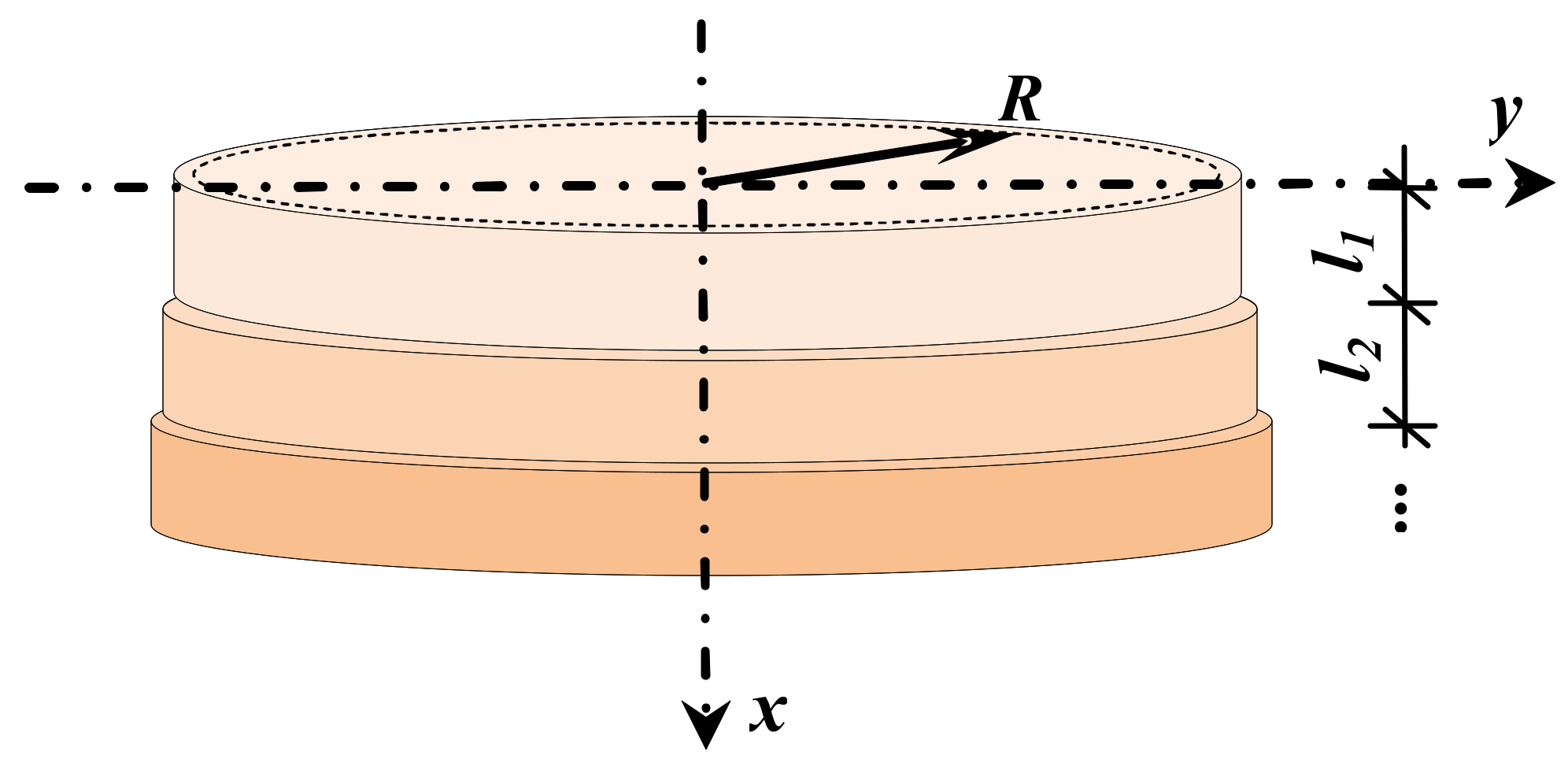
4. Optimal Plastic Design of Shell Composed of Three Rings

In this section, we consider the optimal plastic design of a circular cylindrical full shell composed of three rings. The ring thicknesses are e₁ and e₂ were e₂ ≥ e₁. The shell is subjected to an axially symmetric radial uniform pressure distribution p₀ and no end load. The shell is simply supported. Assuming the perfect plasticity, the dimensioning will use Hodge’s yield hexagon for cylindrical shells. The thicknesses e₁ and e₂ of the rings should be determined so that the shell is on the verge of collapse due to the given limit load p₀ and with total minimum volume. The mechanism of shell collapse is presented in Figure 5.

Dimensioning. Based on the method for obtaining the required thicknesses e₁ and e₂ in the static part, we start with the equilibrium equations of the shell, assuming that the shell is on the verge of collapse. According to the plastic regime on Hodge’s yield condition and expression for moments, we used fracture mechanics, support conditions, symmetry, and the fact that plastic hinges formed in the cross-section, between the rings, are on the side of the ring with smaller thickness e₁.

Thus, six equations from which we determined the unknown ring thicknesses e₁ and e₂ and the unknown constants for the bending moments $M_x^{\left(1\right)}$ and $M_x^{\left(2\right)}$ on the part of the ring e₁ and e₂, respectively, were obtained. In addition to these six equations, we also have the equation of the relationship between the moments of plasticity of the rings. So, in these seven equations, we have seven unknowns.

4.1. Statically Admissible Solution

Based on the static boundary conditions, the continuity of the section forces, and the conditions of symmetry, we obtained the following six equations

$$\begin{array}{l}x=0;M_x^{(1)}=0; \\ x=x_1;M_x^{(1)}=-\xi M{p}_2;\\ x=x_1;\frac{d{M}_x^{(1)}}{dx}=\frac{d{M}_x^{(2)}}{dx};\\ x=x_1;M_x^{(2)}=-\xi M{p}_2; \\ x=x_2=L;M_x^{(2)}=-M{p}_2;\\ x=x_2=L;\frac{d{M}_x^{(2)}}{dx}=0.\end{array}$$

(25)

Using Hodge’s yield condition and Table 11-3 in [21] (p. 277) to our case under consideration, we can obtain for bending moment $M_{{}_x}^{\left(i\right)}$, normal force $N_{\theta }^{\left(i\right)}$, and displacement rate ${\dot{w}}_x^{\left(i\right)}$, as follows

$$M_{{}_x}^{\left(i\right)}=\frac{{\sigma }_0{e}_i^2}{2}\left(D_3^{\left(i\right)}\sin {\omega }^{\left(i\right)}x+D_4^{\left(i\right)}\cos {\omega }^{\left(i\right)}x+\overline{p_0}-1\right),$$

(26)

$$N_{\theta }^{\left(i\right)}={\sigma }_0{e}_i\left(D_3^{\left(i\right)}\sin {\omega }^{\left(i\right)}x+D_4^{\left(i\right)}\cos {\omega }^{\left(i\right)}x+{\overline{p}}_0\right),$$

(27)

$${\dot{w}}_x^{\left(i\right)}=D_1^{\left(i\right)}\sin {\omega }^{\left(i\right)}x+D_2^{\left(i\right)}\cos {\omega }^{\left(i\right)}x,$$

(28)

where $D_1^{\left(i\right)}$$D_2^{\left(i\right)}$ and are the constants and ${\omega }^{\left(i\right)}$ is a parameter from (9). Using the parameter ξ, the relationship moments of plasticity of rings $M_{px}^{\left(i\right)}=\frac{{\sigma }_0{e}_i^2}{4}, (i=1,2)$ is defined by

$$\xi \cdot M_{px}^{\left(2\right)}=M_{px}^{\left(1\right)}, \mathrm{i}.\mathrm{e}.,\xi \cdot e_2^2=e_1^2.$$

(29)

The system Equations (25) with (26) and (29) reads

$$\begin{array}{cc}& \frac{{\sigma }_0{e}_1^2}{2}\left(D_3^{\left(1\right)}\sin {\omega }^{\left(1\right)}x+D_4^{\left(1\right)}\cos {\omega }^{\left(1\right)}x+{\overline{p}}^{\left(1\right)}-1\right)=0;\hfill \\ & \frac{{\sigma }_0{e}_1^2}{2}\left(D_3^{\left(1\right)}\sin {\omega }^{\left(1\right)}{x}_1+D_4^{\left(1\right)}\cos {\omega }^{\left(1\right)}{x}_1+{\overline{p}}^{\left(1\right)}-1\right)=-\xi \frac{{\sigma }_0{e}_2^2}{4};\hfill \\ & \frac{{\sigma }_0{e}_1^2}{2}{\omega }^{\left(1\right)}\left(D_3^{\left(1\right)}\cos {\omega }^{\left(1\right)}{x}_1-D_4^{\left(1\right)}\sin {\omega }^{\left(1\right)}{x}_1\right)=\frac{{\sigma }_0{e}_2^2}{2}{\omega }^{\left(2\right)}\left(D_3^{\left(2\right)}\cos {\omega }^{\left(2\right)}{x}_1-D_4^{\left(2\right)}\sin {\omega }^{\left(2\right)}{x}_1\right);\hfill \\ & \frac{{\sigma }_0{e}_2^2}{2}\left(D_3^{\left(2\right)}\sin {\omega }^{\left(2\right)}{x}_1+D_4^{\left(2\right)}\cos {\omega }^{\left(2\right)}{x}_1+{\overline{p}}^{\left(2\right)}-1\right)=-\xi \frac{{\sigma }_0{e}_2^2}{4};\hfill \\ & \frac{{\sigma }_0{e}_2^2}{2}\left(D_3^{\left(2\right)}\sin {\omega }^{\left(2\right)}{x}_2+D_4^{\left(2\right)}\cos {\omega }^{\left(2\right)}{x}_2+{\overline{p}}^{\left(2\right)}-1\right)=-\frac{{\sigma }_0{e}_2^2}{4};\hfill \\ & \frac{{\sigma }_0{e}_2^2}{2}{\omega }^{\left(2\right)}\left(D_3^{\left(2\right)}\cos {\omega }^{\left(2\right)}{x}_2-D_4^{\left(2\right)}\sin {\omega }^{\left(2\right)}{x}_2\right)=0,\hfill \end{array}$$

(30)

where

$${\overline{p}}^{\left(i\right)}=\frac{p_{0}R}{{\sigma }_0{e}_i}, {\omega }^{\left(i\right)}=\sqrt{\frac{2}{e_{i}R}}.$$

(31)

We introduce the dimensionless values

$$P_s=\frac{p_0}{{\sigma }_0},E_i=\frac{e_i}{R},X_i=\frac{x_i}{R}.$$

(32)

The system (30) and (29) contains seven unknown variables e₁, e₂, constants $D_3^{\left(1\right)}$, $D_4^{\left(1\right)}$, $D_3^{\left(2\right)}$, $D_4^{\left(2\right)}$ and the parameter ξ. After eliminating constants, three nonlinear equations with unknowns e₁, e₂, and ξ were obtained

$$\left(\frac{1}{2}-\frac{P_s}{E_2}\right)\cdot \left\{\cos \left[(X_2-X_1)\sqrt{\frac{2}{E_2}}\right]-1\right\}+\frac{\xi }{2}-\frac{1}{2}=0,$$

(33)

$$\left[1-\frac{P_s}{E_1}-\frac{\xi }{2}{\left(\frac{E_2}{E_1}\right)}^2\right]\cos \left(X_1\sqrt{\frac{2}{E_1}}\right)-\left(1-\frac{P_s}{E_1}\right)-{\left(\frac{E_2}{E_1}\right)}^2\sqrt{\frac{E_1}{E_2}}\left(0.5-\frac{P_s}{E_2}\right)\cdot \sin \left(X_1\sqrt{\frac{2}{E_1}}\right)\sin \left[\left(X_2-X_1\right)\sqrt{\frac{2}{E_2}}\right]=0,$$

(34)

$$\xi \cdot E_2^2=E_1^2$$

(35)

By introducing $E_1=E_2$, then $X_2=X_1$ and ξ = 1 into (34), this Equation (34) becomes the equation of the shell of constant thickness E₁, i.e.,

$$\left(\frac{1}{2}-\frac{P_s}{E_1}\right)\cos \left(X_1\sqrt{\frac{2}{E_1}}\right)+\frac{P_s}{E_1}-1=0.$$

(36)

To solve this system of nonlinear equations, a numerical procedure was implemented. Knowing that the ratio of moments of plasticity is as in (29) and $E_1\le E_2$, the variable ξ must be in the interval $0\le \xi \le 1$. In a computer program, created according to that procedure, we reduce ξ by a fixed step h. The main program contains two subroutines adopted for the numerical calculation of nonlinear equations. In the first subroutine, we determine E₂ and with this value, we obtain E₁ from (34). By entering the values E₁ and E₂, calculated in the first step, into the main program is it checked whether the condition (35) is met. If this condition is not met, we reduce the initial interval for ξ by the initial step h = 0.1 and n = 10. Then, the procedure is repeated with a new step $h_1=\frac{h}{n}=\frac{1}{n^2}$, etc. We interrupt the procedure $h_m=\frac{1}{n^{m+1}}<\epsilon$. In this way, the statically admissible solutions, E₁ and E₂, were obtained. In Section 5 and Section 6, Example 1, a part of this procedure will be shown.

Knowing the values of E₁, E₂, and ξ, we can calculate the constants $D_3^{\left(i\right)}$ and $D_4^{\left(i\right)}$, (i = 1, 2) from (30). After that, we can calculate the bending moments (26) and the normal forces (27).

4.2. Kinematically Admissible Solution and Optimality Conditions

In this part of the paper, the boundary conditions of the shell (37) and the condition of the compatibility of displacements rates (38) will be used (see Figure 5)

$$x=0;{\dot{w}}_x^{(1)}=0;$$

(37)

$$x=x_1;{\dot{w}}_x^{(1)}={\dot{w}}_x^{(2)}.$$

(38)

The conditions (37) and (38) reads

$$D_1^{\left(1\right)}\sin {\omega }^{\left(1\right)}x+D_2^{\left(1\right)}\cos {\omega }^{\left(1\right)}x=0, (x=0),$$

(39)

$$D_1^{\left(1\right)}\sin {\omega }^{\left(1\right)}{x}_1+D_2^{\left(1\right)}\cos {\omega }^{\left(1\right)}{x}_1=D_1^{\left(2\right)}\sin {\omega }^{\left(2\right)}{x}_1+D_2^{\left(2\right)}\cos {\omega }^{\left(2\right)}{x}_1.$$

(40)

Two equations with four unknown variables $D_1^{\left(1\right)}$, $D_2^{\left(1\right)}$, $D_1^{\left(2\right)}$ and $D_2^{\left(2\right)}$ are obtained, and using (31) and (32) it follows as

$$D_2^{\left(1\right)}=0;$$

(41)

$$D_1^{\left(1\right)}\sin \left(X_1\sqrt{\frac{2}{E_1}}\right)=D_1^{\left(2\right)}\sin \left(X_1\sqrt{\frac{2}{E_2}}\right)+D_2^{\left(2\right)}\cos \left(X_1\sqrt{\frac{2}{E_2}}\right).$$

(42)

Application of Optimum Conditions

The conditions of optimum (18), derived in Section 3. for this case, will take the form

$$\frac{\partial {\mathcal{D}}_1}{\partial e_1}=A_1\frac{d{c}_1}{d{e}_1},$$

(43)

$$\frac{\partial {\mathcal{D}}_2}{\partial e_2}=A_2\frac{d{c}_2}{d{e}_2}.$$

(44)

For a specific cost, we choose c₁ = e₁ and c₂ = e₂, which leads to the shell of minimal volume and minimal weight. From Equations (43) and (44) it follows

$$\frac{\partial {\mathcal{D}}_1}{\partial e_1}=2\pi R{x}_1.$$

(45)

$$\frac{\partial {\mathcal{D}}_2}{\partial e_2}=2\pi R\left(x_2-x_1\right).$$

(46)

By substituting m_x and n_θ from (3) and (4) and ${\dot{k}}_x$, ${\dot{\lambda }}_{\theta }$ and ${\dot{w}}_x$ from (6) and (28) into the expression (5) of the power of dissipation energy of the ring of thickness e₁, $\mathcal{D}$₁ is obtained as

$$\begin{array}{l}{\mathcal{D}}_1=\left(\frac{\pi R{\sigma }_0{e}_1{}^2{\omega }^{\left(1\right)}}{2}+\frac{2\pi {\sigma }_0{e}_1}{{\omega }^{\left(1\right)}}\right)\left[D_1^{\left(1\right)}\cos \left({\omega }^{\left(1\right)}{x}_1\right)-\right.\left.D_2^{\left(1\right)}\sin \left({\omega }^{\left(1\right)}{x}_1\right)\right]-\\ \frac{\pi R{\sigma }_0{e}_1{}^2}{2}\left[D_1^{\left(2\right)}{\omega }^{\left(2\right)}\cos \left({\omega }^{\left(2\right)}{x}_1\right)-D_2^{\left(2\right)}{\omega }^{\left(2\right)}\sin \left({\omega }^{\left(2\right)}{x}_1\right)\right]-\frac{2\pi {\sigma }_0{e}_1}{{\omega }^{\left(1\right)}}{D}_1^{\left(1\right)}.\end{array}$$

(47)

The optimum condition (45) with the dissipation $\mathcal{D}$₁ from (47) becomes

$$\begin{array}{l}{\overline{D}}_1^{(1)}\left[4.5\sqrt{\frac{E_1}{2}}\cos \left(X_1\sqrt{\frac{2}{E_1}}\right)+1.5X_1\sin \left(X_1\sqrt{\frac{2}{E_1}}\right)-3\sqrt{\frac{E_1}{2}}\right]+{\overline{D}}_2^{(1)}\left[1.5X_1\cos \left(X_1\sqrt{\frac{2}{E_1}}\right)-4.5\sqrt{\frac{E_1}{2}}\sin \left(X_1\sqrt{\frac{2}{E_1}}\right)\right]-\\ {\overline{D}}_1^{(2)}{E}_1\sqrt{\frac{2}{E_2}}\cos \left(X_1\sqrt{\frac{2}{E_1}}\right)+{\overline{D}}_2^{(2)}{E}_1\sqrt{\frac{2}{E_2}}\sin \left(X_1\sqrt{\frac{2}{E_2}}\right)-2X_1=0,\end{array}$$

(48)

where the notation for constants ${\overline{D}}_i^{\left(i\right)}$ was introduced

$${\overline{D}}_i^{\left(i\right)}=\frac{{\sigma }_0}{R}{D}_i^{\left(i\right)}, i=1,2.$$

(49)

Due to the symmetry of the shell, only half of it was considered, as well as half of the dissipation $\mathcal{D}$₂ of the central ring. By analogous procedure as for $\mathcal{D}$₁, a dissipation $\mathcal{D}$₂ was obtained

$$\begin{array}{l}{\mathcal{D}}_2=D_1^{\left(2\right)}\left[\frac{2\pi {\sigma }_0{e}_2}{\sqrt{\frac{2}{e_{2}R}}}\right.\cos \left(\sqrt{\frac{2}{e_{2}R}}{x}_2\right)-\frac{2\pi {\sigma }_0{e}_2}{\sqrt{\frac{2}{e_{2}R}}}\cos \left(\sqrt{\frac{2}{e_{2}R}}{x}_1\right)+\frac{\pi R{\sigma }_0{e}_2{}^2}{2}\sqrt{\frac{2}{e_{2}R}}\left.\cos \left(\sqrt{\frac{2}{e_{2}R}}{x}_2\right)\right]+\\ D_2^{\left(2\right)}\left[-\frac{2\pi {\sigma }_0{e}_2}{\sqrt{\frac{2}{e_{2}R}}}\sin \left(\sqrt{\frac{2}{e_{2}R}}{x}_2\right)+\right.\left.\frac{2\pi {\sigma }_0{e}_2}{\sqrt{\frac{2}{e_{2}R}}}\sin \left(\sqrt{\frac{2}{e_{2}R}}{x}_1\right)-\frac{\pi R{\sigma }_0{e}_2{}^2}{2}\sqrt{\frac{2}{e_{2}R}}\sin \left(\sqrt{\frac{2}{e_{2}R}}{x}_2\right)\right].\end{array}$$

(50)

With (50) and the optimality condition (46), the fourth equation (51) was obtained

$$\begin{array}{l}{\overline{D}}_1^{(2)}\left[4.5\sqrt{\frac{E_2}{2}}\cos \left(X_2\sqrt{\frac{2}{E_2}}\right)-3\sqrt{\frac{E_2}{2}}\cos \left(X_1\sqrt{\frac{2}{E_2}}\right)\right.+\left.1.5X_2\sin \left(X_2\sqrt{\frac{2}{E_2}}\right)-X_1\sin \left(X_1\sqrt{\frac{2}{E_2}}\right)\right)+\\ {\overline{D}}_2^{(2)}\left(3\sqrt{\frac{E_2}{2}}\sin \left(X_1\sqrt{\frac{2}{E_2}}\right)-4.5\sqrt{\frac{E_2}{2}}\sin \left(X_2\sqrt{\frac{2}{E_2}}\right)\right.+\left.1.5X_2\cos \left(X_2\sqrt{\frac{2}{E_2}}\right)-X_1\cos \left(X_1\sqrt{\frac{2}{E_2}}\right)\right]-2\left(X_2-X_1\right)=0.\end{array}$$

(51)

The system of the linear Equations (41), (42), (48) and (51) is simply to solve and calculate the unknown constants ${\overline{D}}_1^{\left(1\right)}$, ${\overline{D}}_2^{\left(1\right)}$, ${\overline{D}}_1^{\left(2\right)}$ and ${\overline{D}}_2^{\left(2\right)}$. Finally, the displacements rates ${\dot{w}}_x^{\left(1\right)}$ and ${\dot{w}}_x^{\left(2\right)}$ can be obtained by

$${\dot{w}}_x^{\left(i\right)}=D_1^{\left(i\right)}\sin {\omega }^{\left(i\right)}x+D_2^{\left(i\right)}\cos {\omega }^{\left(i\right)}x,\hspace{1em}\left(i=1,2\right),$$

(52)

and the collapse mechanism is determined. In this way, a complete solution in the sense of the theory of limit analysis, including the statically and kinematically parts, can be determined.

5. Numerical Examples

A full cylindrical shell composed of rings of different thicknesses is simply supported and subjected to the uniform internal pressure p₀, as in Figure 2. The following initial data as dimensionless values are given as ring length X₁, then X₂, and $P_s=p_0/{\sigma }_0$. The values of optimal ring thicknesses E₁ and E₂ were determined according to the procedure given in Section 4.

Example 1.

In this example, the dimensioning of the shell is calculated with the given data X₁ = 0.08, X₂ = 0.16, and P_s = 0.035. In the applied numerical procedure, the process is interrupted with the criterion of achieved accuracy$\epsilon =0.0001$.

Table 1. Last iteration for ξ of the numerical procedure.

ξ	E2	E1	ξ∙E2∙E2	E1∙E1	VOLUME
0.7429	0.03073	0.02635	0.000701410	0.000694219	0.004566007
0.7428	0.03072	0.02636	0.000701118	0.000695064	0.004566942
0.7427	0.03071	0.02638	0.000700826	0.000695907	0.004567874
0.7426	0.03071	0.02640	0.000700534	0.000696753	0.004568809
0.7425	0.03071	0.02641	0.000700242	0.000697590	0.004569744
0.7424	0.03071	0.02643	0.000699947	0.000698453	0.004570687
0.7423	0.03070	0.02644	0.000699653	0.000699302	0.004571624
0.7422	0.03070	0.02646	0.000699363	0.000700150	0.004572559
0.7421	0.03069	0.02648	0.000699072	0.000700999	0.004573497

shows the last iteration in which ξ was varied in the interval (0.743; 0.742) with$n=10$.

The step in that iteration was h₃ = 10⁻⁴ and the numerical procedure was completed when ε = 0.0001 was reached. For ξ = 0.7422, the ring thicknesses E₁ = 0.02646 and E₂ = 0.0307 were calculated. The minimum volume is $\overline{V}=0.009145$ where it is $\overline{V}=\frac{V}{2\pi R^3}$. The displacement rates ${\dot{w}}_i$ (i = 1, 2) and its slopes P_i (i = 1, 2) corresponding to the circular plastic hinges of the shell collapse mechanism were calculated (see

Table 2. The strain rate velocities and their slopes.

X1	${\dot{\mathit{w}}}_1$	X2	${\dot{\mathit{w}}}_2$
0.00000000	0.00000000	0.08000000	−17.97580596
0.00800000	−1.94955594	0.08800000	−19.08173715
0.01600000	−3.88968472	0.09600000	−20.108173715
0.02400000	−5.81100477	0.10400000	−21.05072739
0.03200000	−7.70422548	0.11200000	−21.90557981
0.04000000	−9.56019208	0.12000000	−22.66913126
0.04800000	−11.36992999	0.12800000	−23.33819928
0.05600000	−13.12468814	0.13600000	−23.90999527
0.06400000	−14.81598132	0.14400000	−24.38213601
0.07200000	−16.43563122	0.15200000	−24.75265364
0.08000000	−17.97580596	0.16000000	−25.02000388
X1	P1	X2	P2
0.000	−244	0.08	−136
0.08	−187	0.16	−22

).

In this way, the kinematic part of the solution of this example is satisfied.

Bearing in mind that dimensionless quantities were taken into account in the calculation, we assume that it is σ₀ = 235 Mpa and the radius of the shell R = 2 m. The thickness of the ring near the support is e₁ = 52.92 mm, the thickness of the central ring is e₂ = 61.4 mm, and imposed limit load p₀ = 8.225 Mpa.

Example 2.

The following examples show the results of the optimal design of two shells with rings of different lengths, subjected by the same limit load$p_0=0.0345{\sigma }_0$. The data for the first shell is X₁ = 0.085 and X₂ = 0.17 and for the second X₁ = 0.09 and X₂ = 0.18. In the upper part of

Table 3. The calculated thicknesses of optimal shells.

	Ps = 0.0345
X1	0	0.09	0	0.085
X2	0.18	0.18	0.17	0.17
E1	-	0.02861	-	0.02755
E2	0.0321	0.033	0.031	0.0321
	Ps = 0.035
X1	0	0.07	0.095	0.11
X2	0.19	0.19	0.19	0.19
E1	-	0.02638	0.02961	0.03096
E2	0.0332	0.034	0.0345	0.0344

, we represent the calculated thicknesses of these shells E₁ and E₂ and case when X₁ = 0 for the shells of constant thicknesses E = E₂.

Example 3.

The examples of the shells with the same limit load$P_s=0.035{\sigma }_0$and the same length$\overline{L}=2X_2$, but different ring lengths, were calculated (See Table 3, lower part). The following data for X₁: 0 (the shell of constant thickness); 0.7; 0.095 and 0.11 have been taken. Comparing these shells, we conclude that the shell with a constant thickness has a maximum volume,$\overline{V}=0.012616$.

6. Results and Discussion

Performing the structural optimization, the objective function is chosen to be connected with the variables of dimensioning, i.e., the ring thicknesses e₁ and e₂. It was necessary for optimization to be connected with the determination of the minimum of energy and total power of dissipation energy of rings of the shell that the conditions of optimum, derived in Section 3, provide. Through the limit analysis, the greatest resistance of the shell is used. While the shell is operating at the limits of its resistance, we perform a variation of the variable dimensioning, during the derivation of the condition of optimum, to reach the minimum of the energy of dissipation. Thus, the “best” solution that works with the least material under the limit load p₀ was determined. In the condition of optimum, the total power of dissipation energy depends only on bending moments M_x, M_px, normal forces N_θ, N_p, and on-field of displacement rates ${\dot{w}}_x^{\left(i\right)}$ which characterize the collapse mechanism.

In the optimal plastic design (Section 4), both analytical and numerical approaches are exposed. To solve this nonlinear problem (Equations (33)–(35)), we start from the fact that it is real and practical. For approximate initial values, the thickness e from the shell of constant thickness was used, as well as the condition $e_1\le e_2$. Thus, the initial value of E₂ of the central ring thickness was chosen in the subroutine as very small in relation to the shell of constant thickness e. As the number of steps increases, the interval in which the unknown E₂ is located occurs. The determination of the thickness E₁ was carried out in a similar way. As explained in Section 4.1, the main program decreases the interval of parameter ξ at the point where the difference $\xi \cdot E_2^2-E_1^2$ from (35) change sign and specifies the new interval of ξ. In Example 1, (Table 1), this change in sign would be between ξ = 0.7423 and ξ = 0.7422. In this particular case, the interval is reduced because accuracy is required; ε = 0.0001 is reached and this procedure is interrupted.

Based on the same Example 1 and Table 2, a diagram of the displacement rates ${\dot{w}}_x^{\left(i\right)}$ as well as the slopes, i.e., tangents, on the plastic hinges are shown (see Figure 6). Thus, the collapse mechanism of this shell was verified.

In Example 3, three shells with rings were considered. Although each of these shells with rings for a set value of length X₁ is optimal in the plastic range, its gains of volumes (and weights) in relation to the shell of constant thickness are different as follows: for X₁ = 0.07, g₁ = 6.43539%; for X₁ = 0.095, g₂ = 3.571987%; for X₁ = 0.11, g₃ = 2.4425%.

The minimal volume, (i.e., the weight) was obtained for a shell with ring length X₁ = 0.07. We conclude that by choosing the length X₁ we can obtain a generally optimal volume, i.e., the optimal weight for the imposed limit load.

7. Conclusions

• The necessary and sufficient conditions of the optimum for the full circular cylindrical shell with technological limitations, composed of rings of variable thicknesses have been derived with one behavioral constraint related to a specific constitutive low, for limit load-carrying capacity p₀. The paper proves that the necessary optimality conditions are identical to the sufficient conditions of the optimum. The objective function is cost C. The specific cost c_i is the function of thickness e_i which leads to the shell of minimal volume, and also minimal weight. These conditions are derived for a more complex case, i.e., for a full shell with technological constraints, not a sandwich-type shell. Note that in [23], Schielld was the first to derive optimal conditions in the plastic region for a sandwich-type shell, whose thickness can vary continuously from zero to infinity.
• The optimal structural design of shell (in detail with three rings) with an analytical approach complemented by numerical tools and direct connection with basic equations of limit analysis (Section 2) is given. In the static part, the problem is reduced to three linear Equations (33)–(35) and the procedure for their numerical solution is briefly explained, which leads to the optimal dimensions of the shell. Within the kinematic part, the energy dissipation of rings ${\mathcal{D}}_1$ and ${\mathcal{D}}_2$ were analytically obtained, and, using the optimum conditions, the displacement rates of the shell ${\dot{w}}_x$ were determined. In this way, the real collapse mechanism is defined with a minimum of dissipative shell energy. This numerical procedure was applied, and the dimensions in numerical examples were obtained.
• In numerical examples, the optimal dimensions of shells were successfully calculated, applying the conditions of optimum derived in Section 3. Due to the choice of the cost function C, $c_i=e_i$, the shells have minimum volume. In Example 1, the collapse mechanism is shown and confirmed (see Figure 6). For shells of the same limit load p₀ and the same length L, the length of ring X₁ is varied. By comparing these shells, for technological reasons, composed of three rings, with an optimal shell of constant thickness, a gain of 6.4% was achieved. This gain was for the shell of length X₁ = 0.07. By further calculation, the most favorable length X₁ can be obtained.
• This type of cylindrical shell constituted of rings is common in the mechanical, chemical industry, etc. With the increase in the number of rings, the gains also increase. Due to complexity, there are very few solutions to this problem given in analytical, closed-form, and only for simple cases with the results of strongly simplifying assumptions are obtained. The solutions in this paper, which are mostly analytical and complemented by exposed numerical tools, can be useful for confirming numerical procedures, as well as providing information for creating concepts and ideas for technological solutions to more practical and complex problems.
• In further work, this problem will be extended, especially, to the cases of shells with stiffeners, then with end loads for more complex problems of stability and dynamics from practice. Based on the results presented in this paper, the shells, differing in terms of the limit conditions, types of loads, and the number of rings of various thicknesses may be the object of new research and experimental verification to obtain new results.

References

1. Farshad, M. Design and Analysis of Shell Structures; Springer: Berlin/Heidelberg, Germany, 2010. [Google Scholar]
2. Farkas, J.; Jarmal, K. Optimum Design of Steel Structures; Springer: Berlin/Heidelberg, Germany, 2013. [Google Scholar]
3. Kouam, M. Contribution a L’analyse Limite eau Dimensionnement Optimal des Coques Cylindriques. Ph.D. Thesis, Faculte Polytechnique, Palaiseau, French, 1983. [Google Scholar]
4. Caseiro, J.F.; Andrade-Campos, A. An Evolutionary-Inspired Optimization Algorithm Suitable for Solid Mechanics Engineering Inverse Problems. Int. J. Mechatron. Manuf. Syst. 2011, 4, 415–440. [Google Scholar] [CrossRef]
5. Rocha, T.M.; Meireles, J.F.; Pinho, A.C.; Ambrósio, J.A. Update of Coarse Finite Elements Structural Models for Dynamic Analysis Identified from Reference Responses. Int. J. Mechatron. Manuf. Syst. 2011, 4, 402–414. [Google Scholar] [CrossRef]
6. Save, M.; Igić, T. Examples of double-purpose optimal beams. J. Theor. Appl. Mech. 1982, 1, 311–321. [Google Scholar]
7. Save, M.; Prager, W. Structural Optimization, Vol. 1. Optimality Criteria; Plenum Press: New York, NY, USA, 1985. [Google Scholar]
8. Karpat, F. A Virtual Tool for Minimum Cost Design of a Wind Turbine Tower with Ring Stiffeners. Energies 2013, 6, 3822–3840. [Google Scholar] [CrossRef] [Green Version]
9. Radu, D.; Sedmak, A.; Sedmak, S.; Dunjić, M. Stress Analysis of Steel Structure Comprising Cylindrical Shell with Billboard Tower. Teh. Vjesn. 2018, 25, 429–436. [Google Scholar] [CrossRef] [Green Version]
10. Cui, J.; Zheng, Y.; Ohsaki, M.; Luo, Y. Shape Optimization of Piecewise Free-form grid Surface using Plate Components. Eng. Struct. 2021, 245, 112865. [Google Scholar] [CrossRef]
11. Krejsa, M.; Seitl, S.; Brozovsky, J.; Lehner, P. Fatigue damage prediction of short edge under various load: Direct Optimized Probabilistic Calculation. In Proceedings of the 2nd International Conference on Structural Integrity, ICSI 2017, Funchal, Portugal, 4–7 September 2017. [Google Scholar]
12. Wang, D.; Qin, X.; Chen, W.; Wang, S. Simulation of the Deformation and Failure Characteristics of a Cylinder Shell under Internal Explosion. Appl. Sci. 2022, 12, 1217. [Google Scholar] [CrossRef]
13. Hamouche, W. Contrôle de Forme de Coques Multi stables: Modélisation, Optimisation et Miseen Œuvre. Ph.D. Thesis, Université Pierre et Marie Curie Paris VI, Paris, France, 2016. [Google Scholar]
14. Fraldi, M.; Guarracino, F. An Improved Formulation for the Assessment of the Capacity Load of Circular Rings and Cylindrical Shells under External Pressure. Part1. Analytical derivation. Thin-Walled Struct. 2011, 49, 1054–1061. [Google Scholar] [CrossRef]
15. Ambati, M.; Kiendl, J.; DeLorensis, L. Isogeometric Kirchhoff-Love Shell Formulation for Elasto-Plasticity. Comput. Methods Appl. Mech. Eng. 2018, 340, 320–339. [Google Scholar] [CrossRef]
16. Tokarev, A.S.; Karetnikov, D.V.; Fayrushin, A.M. Determining Optimal Geometric Dimensions of Alternative Design Elements of Rolled and Welded Tube-to-Tube Sheet Joints. In Proceedings of the International Conference on Industrial Engineering (ICIE2020), Sochi, Russia, 18–21 May 2020; pp. 227–233. [Google Scholar]
17. Filatov, V.H. Optimal Design of Single-Layered Reinforced Cylindrical Shells. J. Mech. Eng. 2021, 24, 58–64. [Google Scholar] [CrossRef]
18. Zheng, Y.; Zhang, J.; Ohsaki, M.; Wan, H.; Yang, C.; Luo, Y. Optimization of the rod forces in the reticular support structure of JUNO central detector. Structures 2021, 33, 1645–1658. [Google Scholar] [CrossRef]
19. Bideq, M.; Boussitine, L.; Guerlement, G. Contribution à l’optimisation des coques sphériques par l’analyse limite et les algorithmes génétiques. In Proceedings of the 23ènie Congrès de Méchanique, Lille, France, 28 September 2017; Available online: https://hal.archives-ouvertes.fr/hal-03465803/document (accessed on 1 January 2022).
20. Drucker, D.C. Limit Analysis of the Cylindrical Shells under Axially-symmetric Loading. In Proceedings of the 1st Midwestern Conference Solid Mechanics, Urbana, IL, USA, 24–25 April 1953. [Google Scholar]
21. Hodge, P. Plastic Analysis of Structures; McGraw-Hill: New York, NY, USA, 1959. [Google Scholar]
22. Igić, T.S. Contribution to the Optimum Design of Structures. Ph.D. Thesis, Civil Engineering Faculty, University of Nis, Nis, Serbia, 1980. [Google Scholar]
23. Shield, R.T. On the optimum design of shells. J. Appl. Mech. 1960, 27, 316–322. [Google Scholar] [CrossRef]
Figure 1. Circular cylindrical shell.
Applsci 12 02282 g001
Figure 2. Shell differential element.
Applsci 12 02282 g002
Figure 3. Hodge’s plastic yield condition.
Applsci 12 02282 g003
Figure 4. The cylindrical shell formed by rings.
Applsci 12 02282 g004
Figure 5. The simply supported full shell composed of three rings and shell collapse mechanism.
Applsci 12 02282 g005
Figure 6. The simply supported full shell composed of three rings.
Applsci 12 02282 g006