Abstract
The computational cost of the full-scale flue gas desulfurization (FGD) tower with perforated sieve trays is too high, considering the enormous scale ratio between the perforated hole at the sieve tray and the relevant size of the full-scale tower. As a result, the porous media model is used to replace the complex perforated structure at the sieve tray in this study, which has been validated for the measured data for both the small- and full-scale FGD tower. Under a lower inlet gas volume flow rate, the simulation result of the four-tray tower indicates that the uprising gas flow of high SO2 mass fraction can move along the wall of the tower. This region lacks two-phase mixing and, hence, its desulfurization efficiency is similar to that of empty and one-tray towers under the same flow conditions. However, when the gas volume flow rate increases, the liquid column becomes larger because of the stronger inertial of the uprising gas flow. In this situation, the implementation of the sieve tray suppresses the deflection of liquid flow and provides a better mixing within sieve trays, leading to a noticeable increase in desulfurization efficiency. This study provides insightful information for the design guideline for the relevant industries.
1. Introduction
In order to reduce the environmental acidification of sulfur dioxide (SO2) from the fossil fuel power plants or similar facilities, a flue gas desulfurization (FGD) tower is used to absorb the SO2 component from the exhaust gas before it enters the environments [1,2]. Downward alkaline solution injected from spray nozzles mixes with the upward exhaust gas within the tower [2,3,4]. During the desulfurization process, the gas SO2 dissolves into alkaline solution in aqueous phase to form the sulfurous acid (SO2∙H2O), and the ensuing dissociation produces sulfurous by-products, such as bisulfite (HSO3−) and sulfite (SO32−). The sulfurous species lead to the acidification of the alkaline solution. A higher pH value of the solution from the nozzles can neutralize the severity of acidification and absorb more SO2 before its pH value eventually drops [5].
The setups of the nozzles, guide vane, direction of inlet exhaust gas can have tremendous impacts on the two-phase mixing, which can significantly influence the SO2 removal efficiency. The ideal mathematical model that simplifies the flow conditions with uniform velocity [1,6,7,8] could hardly capture these complex geometric effects within a facility, and hence, the Computational Fluid Dynamics (CFD) technique can provide more insightful information and benefit to optimal design. CFD has already been applied widely to solve the multiphase flow dynamics within the FGD tower [4,5,9,10,11,12,13,14,15,16] and other facilities or processes with relevant fields, such as scrubbers of CO2 emissions [11] and fine particle dust concentrators [17]. Depending on its approach to the interactions between liquid–solid and gas phase, the multiphase flow model can be categorized as an Eulerian–Lagrangian model [9,11,12,13,14] and an Eulerian–Eulerian model [5,10].
The liquid droplets are usually regarded as a dispersed phase in the Eulerian–Lagrangian model with tracking of a large number of particles [18]. The droplet is usually regarded as a parcel which contains the same properties [11,12,19,20,21]. The drag coefficient of the particle is determined by the relative Reynolds number, which is based on the slip velocity between the liquid and solid phase. The drag force of a particle usually feeds back to the continuous phase as two-way coupling [9,14]. The chemical reaction is modelled by dual-film theory, Henry’s Law [11,12,13], and Chilton–Colburn analogy [8]. Under the aforementioned framework, Marocco and Inzoli [9] have simulated the hydrodynamics and chemical reaction for a dispersed liquid droplet within an open spray tower. Eight dissolved species from gas to liquid phase are considered during the desulfurization process, and the deposition and splashing of liquid particle as they hit the wall of tower are handled by an empirical droplet–wall interaction model. Qu et al. [11] evaluated the effect of droplet diameter. A finer diameter benefits the mass transfer but could reduce the uniformity of the liquid–gas flow, and vice versa for a particle of larger diameter. An optimal diameter such as 200 μm was selected based on their simulations. Qu et al. [12] further investigated the flow structures at different region of the tower, and the two-phase mixing is stronger in the middle region that dominates the desulfurization process. The evaporation occurs at the inlet region of the gas phase, which only has minor influence on the desulfurization performance. Xu et al. [13] investigated the CO2 removal efficiency by NH3 solution and the effect of the layout of the nozzle spray. A fraction of upward gas can be allowed to flow downward by the entrainment effect of the downward spraying liquid. An upward spray at a lower altitude can enhance 7% removal efficiency from a downward spray at a higher altitude because the former offers a longer residence time and increases the droplet volume fraction.
As for the Eulerian–Eulerian model, it treats both phases as continuous flow. As the upward gas flow and downward liquid flow have a significant slip velocity, two sets of Navier–Stokes equations are required [5,10]. The two-phase mass and force interaction is modelled similar to that in the Eulerian–Lagrangian model, except all the source terms activate in the continuous phase without summation from the dispersed particles. Gomez et al. [5] used an Eulerian–Eulerian model to simulate the desulfurization process by limestone and oxidation for the production of gypsum in the bottom tank. There are six additional species transport equations to tackle the complex chemical reactions. Depending on the complexity of the geometry of the FGD tower, it can be impractical to solve all the chemical species, which could cause convergence issues and increase computational cost. As a result, instead of solving every transport equation, a prepared chemical database that couples with the flow solver [22] was developed in our previous study [10], which significantly reduces the required number of transport equations.
The implementation of a sieve tray can enhance the uniformity of the flow, which is usually favorable to the operation conditions [5,12,23]. The tray-equipped FGD tower is found to increase the SO2 removal efficiency by 7% compared to the empty tower [24]. The detailed two-phase mixing of a small-scale FGD tower implemented by sieve tray was already simulated in our previous study [5]. The number of the perforated holes at each tray is 300 for this small-scale FGD tower. However, this number exceeds 200,000 for the large-scale FGD tower [4]). Considering the extremely large ratio of hole at tray to height and width of the tower, the computation cost can be very large for simulation of the full-scale tower. As a result, the porous media model [5,25] that replaces the perforated details at the sieve tray is used in this study. The porous media model regards the tray region as a flow domain and compensates for the pressure drop by a momentum sink term. The porous media model has already been found to be able to replace the detailed structures for flow past packed beds, filter papers, and perforated plates [24,25,26,27]. The empirical coefficients of the porous media model can be tabulated from Idelchik [28], and the velocity and pressure for a gas flow past tray tower by using porous media model are very consistent with that with a real perforated structure [4], saving significant computational time from the grid resolution near the trays.
In this study, the two-phase chemical flow model is used together with the porous media model, which further validates the capability of the porous media model to replace the complex structures of the FGD tower. It avoids having a tremendous number of grid points near the regions of sieve trays. The required computational time speeds up by 13 times, and hence, it becomes easier to conduct different designs for the small-scale tower, such as the influences of sieve tray and inlet gas flow rate on the two-phase mixing and the ensuing desulfurization efficiency within the FGD tower. The model replacement can also be extended to the full-scale tower simulations of more practicality. This study provides a reliable and fast computational framework and insightful information for the design guidelines for the FGD tower in the relevant industries.
2. Computational Models
The computational framework is based on an Eulerian–Eulerian two-phase model with Navier–Stokes equations, porous media model, standard k-ε turbulence closure, and species equations. This Eulerian–Eulerian model, chemical reactions, and porous media model are discussed in Section 2.1, Section 2.2 and Section 2.3.
2.1. Eulerian–Eulerian Two-Phase Flow Model
The Favre-Averaged Navier–Stokes model [5,18,22] has been used to account for the density variation between liquid and gas phases, and the Eulerian–Eulerian two-phase model [5,10] is utilized to handle the slip velocity. Two sets of Navier–Stokes equations are solved in this study. For each phase, the continuity in Equation (1) and Navier–Stokes equations in Equation (2) based on the Eulerian–Eulerian model are presented as follows:
In Equations (1) and (2), the gas and liquid phases are represented by the subscripts g and l, respectively, and the subscripts i and j are the Einstein notations. The symbol u represents velocity, ρ is density, P is pressure, α is volume fraction, τ is laminar stress, τR is Reynolds stress, G is gravity (9.8 m/s2 in –y direction), Ki is the exchange coefficient, and M is a momentum sink term for the porous media model. For simulation by real perforated structure, the porous media model is not activated.
As shown in Figure 1, air and SO2 gas are the components of gas phase, and the sulfurous slurry and magnesium hydroxide (Mg(OH)2) are the components of liquid phase. The Mg(OH)2 solution removes the SO2 gas phase by absorption, and new chemical by-product, namely sulfurous slurry, is generated in the liquid phase. The SO2 gas is less than 130 ppm, and hence it is reasonable to assume that the corresponding phase change in Figure 1 does not really affect the continuity and momentum equations. Therefore, the source term related to chemical reactions is absent in Equations (1) and (2) [1,5,10,29]
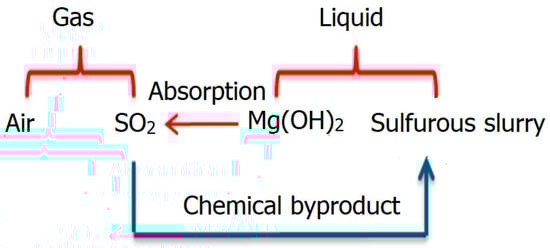
Figure 1.
This schematic shows the components in gas and liquid phases during the desulfurization process.
The symbols ρg and ρl in Equation (3) are the mixture densities for the gas and liquid phases, respectively:
The value of ρg can be calculated from the mass fractions of SO2 and air within the gas phase (YSO2 and Yair) and their densities (ρSO2 = 2.384 kg/m3 and ρair = 1.066 kg/m3). Similarly, ρl is obtained from the mass fractions of slurry and Mg(OH)2 solution within the liquid phase (Yslurry and YM) and the corresponding densities (ρSlurry = 998.2 kg/m3 and ρM = 983 kg/m3).
The laminar stress τ in Equation (2) is based on the Newtonian assumption, which is the product of the velocity gradient and the mixture viscosity μ. The turbulent stress τR in Equation (2) is computed by standard k-ε turbulence model [5,22,30,31]. The turbulent viscosity stems from the empirical relations between turbulence kinetic energy k and turbulent dissipation rate ε. The turbulent stress τR, which utilizes the Boussinesq’s approximation, is also the product of the velocity gradient and the turbulent viscosity.
In Eulerian–Eulerian model, Ki(ug,I − ul,i) in Equation (2) is the i-direction interaction force from liquid to gas phase. As a result, the interaction force from gas to liquid in i-direction is Ki(ul,I − ug,i), which switches the direction but has the same magnitude. Ki is the exchange coefficient of i-direction, and its value can be determined from the empirical relations as follows [6,22,32]:
In Equation (4), f is the drag function, Cd is the drag coefficient, τr is the relaxation time, Rer is the Reynolds number based on two-phase slip velocity and the liquid droplet diameters dl. The size of droplet diameter is chosen as 500 μm in this study from preliminary results, which is also similar to the selection of ref. [11,12].
After chemical reactions, the SO2 within gas phase is reduced, and the slurry is produced in liquid phase, as indicated in Figure 1. This desulfurization process is controlled by Equation (5) with source term S, which will be discussed in the next subsection.
An isothermal temperature around 58 °C is measured within the FGD tower by China Steel Cooperation. Therefore, the energy equation is not activated in this study. Similar situations can be seen in ref. [1,5,10,20,29].
2.2. Chemical Mechanisms
Figure 2 illustrates the chemical reactions during the desulfurization process. In the upper left corner of Figure 2, it indicates that the SO2 gas dissolves into liquid phase and hydrates to form SO2∙H2O. One proton is lost and HSO3− is generated because of the dissociation, and HSO3− has subsequent dissociation to lose another proton and form SO3−2:
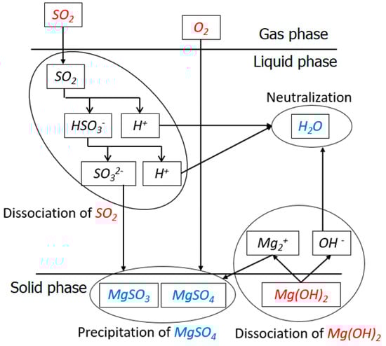
Figure 2.
This schematic illustrates the chemical reactions during the desulfurization process.
The subscript “(aq)” in Equation (6) denotes the aqueous phase. The Mg(OH)2 solution is a strong electrolyte, which can dissociate completely to release magnesium ions (Mg2+) and OH− ions. The neutralization takes place between OH− ions from Mg(OH)2 and H+ ion from Equation (6):
The nonlinear algebraic equations for Equations (6) and (7) can be listed as below:
In Equation (8), K1, K2, and K3 are the equilibrium constants for the corresponding reactions based on 58 °C [5]. The symbol corresponds to the molar concentration (mole/m3) of H+ in the liquid phase l, which can also be applied to the symbols for other species. The sulfurous species, such as HSO3−, SO32−, and SO2 in the liquid phase, are usually added together and regarded as a single variable, as denoted byClSlurry [5,9]:
Moreover, Equation (10) is the charge balance:
As the Mg(OH)2 solution has complete dissociation, the initial value from the spray nozzles is double that of the . Additionally, the value of pH from the nozzles has always been kept as 7.7 in the facility. The value of can be calculated:
In Equation (11), 10−7.7 is the concentration of H+ ion from the inlet of nozzle sprays, and K3 is equilibrium constant for neutralization as shown in Equations (7) and (8). is calculated as 3.08 × 10⁻⁷ mole/m3 from Equation (13). Since Mg2+ does not participate in the chemical reactions, this value is regarded as constant within the flow domain and only has influence on the balance of the electric charge in Equation (10).
Therefore, from Equations (8) to (10), there are six unknowns, , within five equations. The nonlinear algebraic sets of Equations (8)–(10) can be solved numerically once ClSlurry is known. This value can be calculated in Equation (12):
The molecular weight of the slurry phase Wslurry (kg/mole) is 80 in Equation (12) [5,10,33]. Similar to Equation (12), the molar concentration of the SO2 gas, CgSO2, can be obtained as the molecular weight of the SO2 WSO2 = 64:
The chemical source term S in Equation (5) is modelled as follows [5,9,10]:
In Equation (14), Aint is the interfacial contact area per unit volume, which is defined as 6αl/dl. The Henry’s law constant HSO2 is 82. The mass transfer coefficient kgSO2 for SO2 in the gas is 4 × 10⁻⁵ m/s while that in liquid phase (klSO2) is 3.4 × 10⁻⁴ m/s. The enhancement factor ESO2 is 1.3 in this study. All the chemical relevant constants above are taken based on the values of 58 °C [5].
In this study, the flow solver we use is ANSYS Fluent [22]. The computational procedures that couple the flow solver and chemical reactions are described as follows:
- Step 1:
- Solve the Eulerian–Eulerian two-phase flow models from Equations (1) to (5) at the current time step, while the chemical source term S in Equation (14) is obtained from the previous time step.
- Step 2:
- Obtain ClSlurry from Equation (12) and CgSO2 from Equation (13) according to the flow variables of the current time step.
- Step 3:
- Input ClSlurry from Equation (12) into a prepared chemical database by UDF. This database is written in Matlab to solve the sets from Equations (8) to (10). With ClSlurry given from flow solver, this chemical database can solve the remaining unknowns and then output the value of ClSO2 to the flow solver.
- Step 4:
- Insert CgSO2 from step 2 and ClSO2 from step 3 into Equation (14) to calculate a new chemical source term S for the next time step.
- Step 5:
- Update the time step and repeat step 1 to 4 if necessary.
The couple between flow solver and chemical database can avoid too many additional transport equations for species introduced in Figure 2, which can save computational time and reduce the ensuing numerical difficulties [5].
2.3. Porous Media Model
A momentum sink term M, as shown in Equation (2), is activated in the designated porous media region to compensate the pressure loss because the detailed solid boundary is not resolved [4,24,25]:
In Equation (15), the subscript q stands for either gas phase g or liquid phase l, and i represents the direction. Additionally, C represents the inertial loss coefficient, and th is the thickness of the porous media region. The value of inertial loss coefficient in Equation (15) is usually calculated by an empirical equation based on a large number of experimental data [25,26,27,28]. For example, Idelchik [28] provided the inertial loss coefficient C:
In Equation (16), the hole diameter is Dh, and fh is the porosity and defined as the ratio of the total hole area to total area of the plate. The coefficients ξ1, ξ3, ξ4, and λ in Equation (16) can be tabulated based on the porosity fh, hole Reynolds number Reh, and th/Dh, which is the ratio of the tray thickness to the hole diameter. As for Reh, it is defined as ρVDh/fhμ where ρ, V, and μ correspond to values from gas or liquid phases.
3. Validations of the Two-Phase and Porous Media Model
3.1. Geometries of the Small- and Full-Scale FGD
A small-scale pilot FGD tower was used for validation first. Figure 3a illustrates the details of the facility. All the spray nozzles and four sieve trays are set up in the right tower while the left tower is closed in this series of experiments. The height of the tower is 2.4 m, and the diameter is 0.6 m. The spacing between each tray is 0.4 m, and the spray system is placed above the highest tray by 0.2 m as shown in Figure 3a,b. The liquid Mg(OH)2 solution is injected downward without spray angle by 33 nozzles, as arranged in Figure 3b from the top view. The array of nozzles has a radial distance of 0.05 m, and the diameter of each nozzle is 0.01 m. The pH value of liquid Mg(OH)2 solution is 7.7 at the exit of nozzle. The gas with SO2 enters the domain from a pipeline of a diameter 0.4 m in the rightmost face, as shown in Figure 3a. With a series of chemical reactions shown in Section 2.2, the desulfurization process reduces the concentration of SO2, while the sulfurous process increases the acidity of the slurry. The liquid slurry then is discharged through the outlet under the bottom tank. Furthermore, Figure 3b highlights the sampling locations to measure the SO2 removal efficiency. Assuming point P in Figure 3b is the origin in the x–y plane, the locations of the sampling points from GT1 to GT3 are (−0.2, 0.93), (−0.2, 1.345), and (−0.263, 2.16), respectively, with meter as the unit.
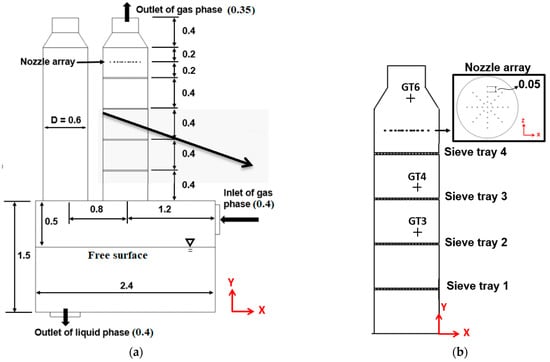
Figure 3.
This figure displays (a) details of the small-scale FGD tower and (b) the layout of the nozzle arrays from the top view with the sampling locations for the SO2 concentration. The unit is meter.
Figure 4 illustrates the full-scale FGD tower. The height and diameter of the tower are 23 and 7 m. The tower has three sieve trays, and the gas is transported by a pipeline with diameter of 3.6 m and it leaves the domain from the outlet with a diameter of 3.6 m. There are two sets of nozzle arrays. One is above the highest tray by 1 m with 192 nozzles, and the other is below the lowest tray by 1.2 m with 29 nozzles. Both sets of nozzles have spray angle of 65°and diameter of 0.05 m. The experiments for both small- and large-scale towers have already been conducted by China Steel Cooperation [34] with measured data for desulfurization and pressure at designated sampling points.
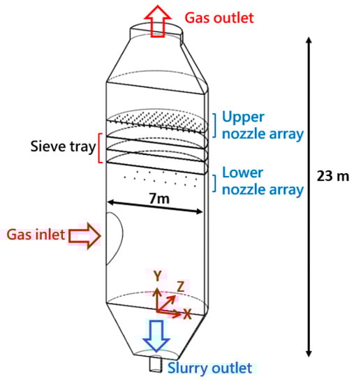
Figure 4.
This figure highlights the details of the large-scale FGD tower. The unit is meter.
3.2. Geometries of the Perforated Sieve Trays of the Small- and Full-Scale FGD
The perforated hole structure on a sieve tray is illustrated in Figure 5 from the top view (left) and side view (right). For the small-scale tower, the important parameters required to determine the inertial loss coefficient C in Equation (16) are listed in Table 1 for different cases and phases. The hole diameter Dh is 20 mm, the tray thickness th is 15 mm, and the pitch Ph is 28.8 mm. With the aligned layout shown in Figure 5, the hole diameter Dh and pitch Ph can determine the porosity fh as 34.3%. The hole Reynolds number for gas phase Reh,g = ρgVgDh/fhμg is 5130, where ρg and μg are the density and dynamic viscosity of the gas phase, and Vg (1.4 m/s) is the cross-sectional average velocity of the gas phase within the tower. L/G is defined as the mass flow rate ratio of the total liquid to the exhaust gas. There are two setups for the small-scale tower, and this value varies as 4.9 or 3.2 for the small-scale tower, namely, Case 1 and 2. For Case 1, the velocity of the liquid solution is 0.766 m/s from each spray nozzle with a diameter of 0.01 m, and the velocity of Case 2 is 0.511 m/s. Similar to gas phase, the hole Reynolds number for liquid phase Reh,l is 860 and 570, respectively.
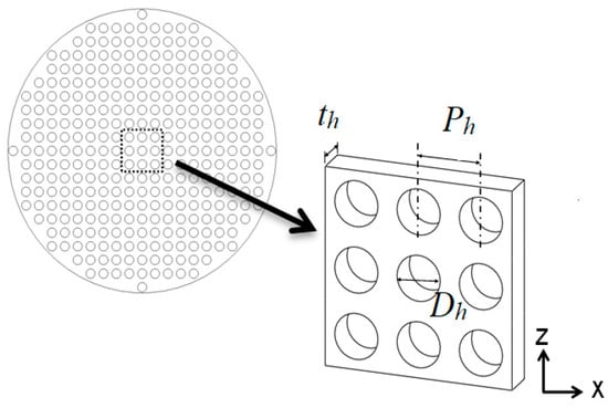
Figure 5.
This figure illustrates the top view of the perforated structure of the sieve tray.

Table 1.
This table displays the important parameters of the sieve tray.
Each sieve tray has 308 holes for the small-scale tower. By using the porous media model in Equation (16), these aforementioned parameters are used to determine the inertial loss coefficient to replace the detailed perforated structures. As for the tray of full-scale tower, its perforated hole is 8 mm. The porosity fh is 27.7%, th/Dh=0.75, the hole Reynolds numbers Reh for liquid and gas phase are 5500 and 940, respectively, which are all similar to those of Case 1 in the small-scale tower. As for the number of holes, there are 200,000 holes at each sieve tray for the large-scale tower.
3.3. Working Conditions of the Small- and Full-Scale FGD
For the small-scale tower, the inlet gas flow Reynolds number, Reinle, is around 8 × 10⁴ according to the gas mixture density (1.067 kg/m3), velocity (3.2 m/s), and the diameter of the pipeline (0.4 m) at the inlet as shown in Figure 3a. With different L/G values, the inlet Reynolds numbers for the liquid are about 1.6 × 10⁴ for Case 1 and 1.07 × 10⁴ for Case 2. These flow conditions of the gas and liquid inlets of the small-scale tower are highlighted in Table 2 and Table 3. Moreover, the concentration of SO2 gas at inlet is 152 and 145 ppm, respectively.
Table 2.
This table highlights the important parameters of inlet flow of Case 1 (L/G=4.9) for the small-scale tower.
Table 3.
This table lists the important parameters of inlet flow of Case 2 (L/G=3.2). for the small-scale tower.
As for the large-scale tower, the Reynolds number at inlets is 6.35 × 10⁵, 1.35 × 10⁵, and 1.44 × 10⁵ for gas at inlet, liquid at the lower, and higher spray array, respectively. The corresponding value of L/G is 5, and the SO2 gas at inlet is 359 ppm.
3.4. Boundary Conditions, Grid Layouts, and Validations for the Small-Scale Tower
Figure 6a illustrates the grid layouts by cut-cell technique [5,22] for the small-scale tower at the symmetric plane at z = 0. Its computational domain is discretized by hexahedral elements with finer resolution around the spray nozzles and sieve trays in Figure 6b. The velocities at inlets for both gas and liquid are prescribed according to Table 2 and Table 3, while the pressure is extrapolated. The turbulent quantities are specified as eddy-to-laminar viscosity ratio equal to 1000. At the gas inlet, the volume fraction of gas phase αg is 1. For Case 1, the concentration of SO2 gas YSO2 at this inlet is 3.42 × 10⁻⁴, converting from the ppm value (152 ppm) and inlet densities. At the liquid inlets, the liquid volume fraction αl and mass fraction YM for the Mg(OH)2 are all set up as 1.
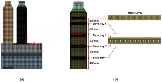
Figure 6.
The figure displays the grid distributions of the small-scale FGD tower at the symmetric plane (z = 0) in (a) and the detailed layouts for the right tower near the sieve trays and nozzles in (b).
The pressure at gas outlet is maintained as 1 atm, while remaining variables are extrapolated. The liquid outlet at the bottom surface of Figure 3a is set up as 1.1 atm, in order to maintain the height of the free surface of the bottom tank by 1 m.
For the simulation by real perforated sieve tray, the no-slip boundary condition is applied to the surface of the sieve tray and wall of the tower. The turbulent quantity k is zero, while ε is calculated by wall function. In this study, the y+ value for the first grid away from the no-slip wall is around 60. As for the porous media model, the tray region becomes an interior flow domain without solid boundary and retains the same grid resolution as that outside the tray.
The nonlinear sets of equations from Equations (1)–(5) are solved by Phase Coupled SIMPLE (PC-SIMPLE) [22,35], which is based on an extension of the SIMPLE algorithm to multiphase flows. The Second Order Upwind scheme (SOU) [22,30] is used for the convective nonlinear terms, and the central difference is applied to diffusion terms. The time step size for small-scale tower is 0.01 s. Although the time-dependent computation is considered, the solution finally reaches a steady state for a small-scale tower.
After a series of grid dependency test, the mesh with number of grid points as 1.2 × 10⁶ is chosen for the further simulations. Table 4 and Table 5 list the simulated SO2 removal efficiencies at three sampling locations for Case 1 (L/G = 4.9) and Case 2 (L/G = 3.2) by real perforated structures. The measured values [36] have also been compared, and the results are consistent with most of discrepancies less than 10%.
Table 4.
This table displays the SO2 removal efficiencies of small-scale tower by numerical and experimental results [36] at different sampling points as L/G = 4.9.
Table 5.
This table displays the SO2 removal efficiencies of small-scale tower by numerical and experimental results [36] at different sampling points as L/G = 3.2.
3.5. Comparisons between Numerical Results by Perforated Structures and Porous Media Model in a Small-Scale Tower
After validation in a small-scale tower, this subsection discusses the feasibility of using porous media model for saving computational cost. Case 1 and Case A have the same flow conditions, except the latter applies the porous media model, and the same situation applies to Case 2 and Case B. Different setups for number of sieve trays and inlet gas flow rate will further be discussed by using the porous media model in Section 4. Table 6 presents the case name, flow condition, parameters in porous media model, and SO2 removal efficiency at outlet for all the different cases.
Table 6.
This table highlights the different cases of small-scale tower that computed by porous media model with SO2 removal efficiencies at outlet.
For the small-scale tower of L/G = 4.9, the hole Reynolds number for gas phase Reh, is 5130, porosity fh is 34.3%, and th/Dh is 0.75 for Case 1, as shown in Table 1. These values are used to tabulate in ref. [28], and obtain values of ξ1= 0.123, ξ3 = 0.658, ξ4 = 0.525, and λ = 0.037 in Equation (16). The inertial loss coefficient in Equation (2) for gas flow in y-direction Cg,y is 11.33 after inserting these values into Equation (16). As for liquid phase in Table 1, the hole Reynolds number for liquid phase Reh,l is 860 for Case 1, corresponding to ξ1 = 0.25, ξ3 = 0.513, ξ4 = 0.525, and λ = 0.074. From Equation (16), the inertial loss coefficient for liquid phase Cl,y is calculated as 10.31.
As the main direction of flow within the perforated hole aligns with the y-direction, the inertial loss coefficients of these two phases in the x- and z-directions are amplified by 100 times from their corresponding values in the y-direction [4,22]. From our preliminary results, based on the aforementioned setups (Cg,y = 11.33 and Cl,y = 10.31) for porous media model, the pressure drop within the right tower of the small-scale tower as L/G = 4.9 is 86.7 Pa, while that computed by real perforated structures (Case 1) is 104.6 Pa. This deficiency by using porous media model is caused by Equation (16) being calibrated based on experiments with single-phase flow [4,25,28] and the two-phase flows within the tower have opposite direction.
As a result, it is reasonable to increase the inertial loss coefficients for the two-phase counterflow. Considering that gas flow occupies most of the domain within the tower, only the value of gas flow Cg,y increases by 33% from 11.3 to 15 after a series of tests. The numerical results of Case A by Cg,y = 15 and Cl,y = 10.31 yields a pressure drop 103.5 Pa, which is exactly the same as that by Case 1 with perforated structures. As for Case B with a lower L/G, the information in Table 1 yields original values of Cg,y = 11.3 and Cl,y = 10.48 from Equation (16). Similar to that for Case A, Cg,y = 11.3 is increased by 33% to Cg,y = 15 while Cl,y is maintained as 10.48. The corresponding pressure drop is 96.8 Pa, which is very consistent to 95.5 Pa of Case 2 by real perforated structures. Therefore, these treatments that increase Cg,y by 33% and retain the original Cl,y are applied to all the simulations by porous media model, as shown in Table 6.
Figure 7 displays the liquid volume fraction (αl), streamlines of gas phase, and the mass fraction of SO2 (YSO2) within the right tower of small-scale FGD facility for Case 1 and Case A at L/G = 4.9. Both cases of perforated structures and porous media model have similar flow patterns. Figure 8 presents the liquid flow velocity (ul,y) and gas flow velocity (ug,y) in the y-direction along the centerline of the small-scale tower for Case 1 and Case A, and the velocity is normalized by average gas velocity Vg (1.4 m/s). The dashed lines display the positions of sieve trays. It is clear that the downward liquid flow in Figure 8a accelerates between each sieve tray and decelerates as the liquid flow approaches the sieve tray.
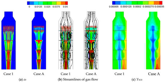
Figure 7.
The figure displays (a) the liquid volume fraction, (b) streamlines of gas flow, and (c) the mass fraction of SO2 within the right tower of the small-scale FGD facility for Case 1 (real perforated structure) and Case A (porous media model).
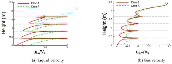
Figure 8.
This figure displays the liquid and gas flow velocity along the centerline of the small-scale tower for Case 1 and A.
For Case A, the porous media model can also obtain a strong deceleration as that in Case 1 with real perforated structures. Since the sieve tray is not regarded as a no-slip boundary condition in the porous media model, the liquid flow cannot decelerate to zero velocity when it impacts the porous-based sieve tray, as shown in Figure 8a. Moreover, the sudden reduction of the cross section within the real perforated sieve tray leads to a very strong acceleration. However, the porous media model regards the sieve tray as an interior flow domain, and hence, the strong acceleration cannot be displayed by Case A in Figure 8a. As a result, the liquid velocity between two sieve trays is slower by using the porous media model in Figure 8a. Considering the extremely large liquid-to-gas density ratio, the gas flow inside the liquid column travels downward with the liquid flow instead of rising, which is illustrated in Figure 8b for gas flow at the centerline of the tower for both cases. Since the liquid flow of Case 1 is faster, as mentioned previously in Figure 8a, it can accelerate the gas flow into a faster velocity. Correspondingly, the gas flow velocity between two sieve trays is made slower by using the porous media model in Figure 8b.
Since the liquid flow decelerates to zero as it approaches the sieve trays for Case 1 as shown in Figure 8a, it tends to accumulate at each top surface of sieve tray, as shown in Figure 7a. As for the porous media model of Case A, although the liquid flow cannot decelerate to zero velocity onto the sieve tray, it remains sufficient to hold the liquid flow and produce accumulation near the locations of sieve trays.
In contrast with the downward gas flow within the liquid column, the gas flow outside it moves upward, which can be seen in the streamlines in Figure 7b. As a result, the liquid column serves as a boundary to separate the upward and downward gas flow, and hence, a pair of counter vortexes between two neighboring sieve trays can be seen in Figure 7b for both cases. The radius of liquid column can be extracted from Figure 7a, which defines the size occupied by liquid flow. Figure 9 illustrates the radius as function of y-direction for Case 1 and Case A. The trend is comparable with average deficiency as 15% between Case 1 with perforated structure and Case A by porous media model.
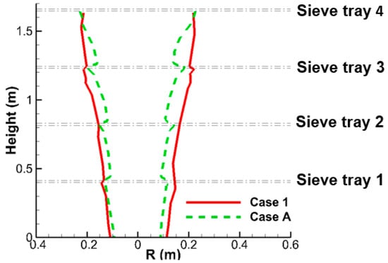
Figure 9.
This schematic shows the radius of liquid column of the small-scale tower for Cases 1 and A.
Since the two-phase flow structures are comparable for both cases, as shown in Figure 7a,b, Figure 8 and Figure 9, the mass fraction of SO2 (YSO2) in Figure 7c also has similar trends. Table 4 and Table 5 further compare the SO2 removal efficiencies at different sampling points, which also displays similar trends and values between perforated structures (Case 1 and Case 2) and porous media models (Case A and B). Most important of all, the number of grid points after the sensitivity test for Case A and Case B is only 2 × 10⁵, which is one-sixth that of Case 1 and Case 2. As a result, the computational time is reduced significantly from 8 days to 15 h (32 cores with 3.82 GHz processer), which makes it easier to conduct different designs as Case C–G for the small-scale FGD tower in Table 6.
3.6. Numerical Results by Porous Media Model in a Large-Scale Tower
A mesh with number of grid points 1.2 × 10⁶ is required for a small-scale tower that has 1200 holes at those four sieve trays. As for the large-scale tower, the number of holes becomes 600,000, and it could require a mesh of six hundred million grid points if their resolutions remain the same. The previous subsection validated the feasibility of the porous media model in a small-scale tower, which has also been utilized for the large-scale tower in this study to save computational costs. The number of grid points for the large-scale tower is 8 × 10⁵ with the porous media model near the sieve trays.
The size and flow conditions of the large-scale tower were introduced in Figure 4, Section 3.1 and Section 3.3. The setup of the boundary conditions is the same as that for the small-scale tower in Section 3.4. The characteristics of perforated sieve trays used in the large-scale tower are fh = 27.7%, th/Dh = 0.75, Reh,g = 5500, and Reh,l = 940, corresponding to Cg,y = 18.41 and Cl,y is 17.3 from Equation (16). By comparing with the measured pressure drop as 901 Pa in the experiment, the inertial loss coefficient of gas Cg,y is adjusted 3 times from 18.41 to 73.3, while Cl,y remains 17.3 to compensate the effects of two-phase counter flow as mentioned previously in Section 3.5. After these treatments, the pressure drop calculated by the porous media model is 892 Pa, which is very close to the measured data. The simulation result displays unsteady flow structures, and is illustrated in Figure 10a,b with time step size as 0.05 s. The two-phase mixing is very strong within the tray regions in Figure 10a, resulting in a significant reduction of SO2 mass fraction from the inlet, as shown in Figure 10b.
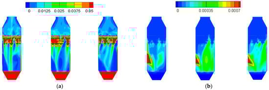
Figure 10.
The figure displays (a) the liquid volume fraction and (b) the mass fraction of SO2 (YSO2) for the large-scale tower at different times, by the porous media model.
Figure 11 shows the instantaneous variation of mass fraction of SO2 (YSO2) at outlet for the full-scale tower. The value of YSO2 varies between 4 and 11 ppm, corresponding to SO2 removal efficiency of 97–98.9%. The average efficiency is 98.3%. The experiment of this large-scale tower by China Steel Cooperation reports the efficiency as 96%. Therefore, this subsection further validates the porous media model in the full-scale tower.
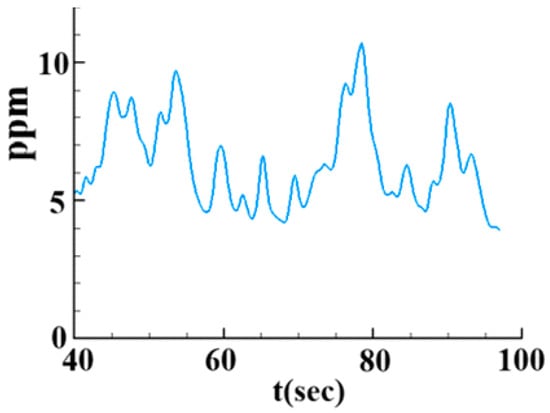
Figure 11.
The schematic shows the instantaneous variation of mass fraction of SO2 (YSO2) at outlet for the full-scale tower.
4. Designs of the Small-Scale Tower from Numerical Experiments
4.1. Comparisons between Four-Tray and Empty Tower (Case A and Case C)
Case C has the same flow conditions (L/G = 4.9) as Case A, except all the sieve trays are removed. Figure 12a,b shows the liquid flow structures by αl and gas flow structure by streamlines for Cases A and C. As the implementation of sieve trays can provide deceleration of the liquid phase as it approaches the sieve tray, the liquid phase of Case A is apparently much denser at the tray locations than for Case C in Figure 12a. The gas flow within the liquid column of Case C remains downward because of the large liquid-to-density ratio. Instead of several pairs of counter vortexes, as shown in Figure 12b for Case A, the downward gas flow only forms one larger pair of counter vortexes with the uprising gas flow outside the liquid column. Therefore, the complex flow structure of Case A in Figure 12b can enhance the two-phase mixing and the ensuing chemical reactions in Equations (6)–(8) more efficiently. As a result, the SO2 mass fraction within the liquid column of Case A is lower than that of Case C in Figure 12c.
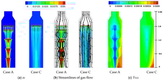
Figure 12.
The figure displays (a) the liquid volume fraction, (b) streamlines of gas flow, and (c) the mass fraction of SO2 within the right tower of a small-scale FGD facility for Case A and Case C (empty tower).
However, from Table 6, the SO2 removal efficiency at outlet of Case C (56.9%) is very close to that of Case A (57.1%), which seems to be inconsistent with previous results shown in Figure 12c. The contradiction can be explained in Figure 13. Figure 13 shows the top view of SO2 mass fraction at different cross sections as y = 0.615 and 2.46 m from Figure 12c. The SO2 mass fraction is indeed lower for Case A near the center where the liquid column passes through, but there exists a high SO2 region to the right of the lateral at each cross section. This trend can also be seen in Figure 12c for Case A near the right wall, which is related to the size of liquid column and explained as follows.
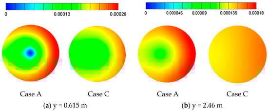
Figure 13.
This schematic shows the mass fraction of SO2 (YSO2) at different cross sections from top view for Case A and Case C.
Figure 8 above displays the deceleration of liquid flow near the top surface of each sieve tray and acceleration as liquid flow penetrates it. Furthermore, the dilute liquid flow can accumulate into a denser liquid column by using sieve trays, as shown in Figure 7a. As a result of the continuity, the deceleration enlarges the region of the liquid column, while the acceleration reduces it. This trend can be seen every time the liquid column passes the tray regions from their top to bottom surfaces in Figure 9. Figure 8 further indicates that the velocity of liquid flow has not reached its terminal velocity between each sieve tray, which implies that the acceleration remains even after the tray region. As a result, the size of the liquid column keeps decreasing in the region between two trays. These aforementioned mechanisms result in a continuous reduction of the radius of liquid column, as shown in Figure 9.
Without a sieve tray, the liquid flow fails to accumulate to form a liquid column with a higher liquid volume fraction. The liquid column resembles several different discrete liquid flows. This scatter characteristic makes its variation in size less sensitive to the y-direction. The radius of liquid column is almost decided by the radial location of the outermost nozzle spray shown in Figure 3b. As a result, the radius of the liquid column of Case A is reduced more rapidly than that of Case C in Figure 12a, which is further illustrated in Figure 14 in the y-direction. The size of the liquid column is apparently larger for Case C without sieve tray.
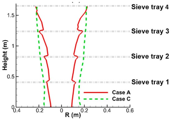
Figure 14.
This schematic shows the radius of liquid column of the small-scale tower for Cases A and C.
The region outside the liquid column is the uprising gas flow. It is basically located around the wall of tower with poor two-phase mixing and corresponds to a region of high SO2 mass fraction. Therefore, the narrower liquid column for Case A incurs a larger area of uprising gas flow with high SO2 mass fraction than that in Case C, as illustrated in Figure 12c and Figure 13. Moreover, one can see that the distributions of high SO2 regions are not symmetric. As the inlet of gas flow is at the right side of the tower as shown in Figure 3a, a portion of the gas flow has already encountered the liquid column at the region of y < 0 in Figure 3a before it enters the left side of the tower as y > 0. Consequently, the SO2 mass fraction is higher on the right side than on the left side of the tower, as shown in Figure 13.
To sum up, although the two-phase mixing within the liquid column for Case A is better than that of Case C in Figure 12c, the narrower liquid column in Figure 14 produces a larger area with high SO2 mass fraction when the four sieve trays are implemented. These two competing effects end up with very comparable SO2 removal efficiencies at outlet, as listed in Table 6 (57.1% and 56.9%).
4.2. Comparisons between Empty and One-Tray Tower (Case C and Case D)
As shown in Table 6, Case D has the same flow conditions (L/G = 4.9) as Case A and C, except only the lowest sieve tray is implemented, as shown in Figure 15a. Figure 15a,b shows the liquid flow structures for Cases C and D. Before the liquid flow reaches the lowest sieve tray, Cases C and D have consistent size of liquid column, as shown in Figure 15a and Figure 16. Moreover, the liquid flow reaches the terminal velocity 4.2 m/s at y = 0.75 m for both cases, and this stronger inertia causes a more obvious deflection when it impacts the lowest sieve tray for Case D, as highlighted in Figure 16. Although the liquid column becomes smaller after the lowest sieve tray, as discussed previously, the deflection makes the reduction from a wider liquid column. This results in a larger liquid column for Case D than Case C in Figure 16.
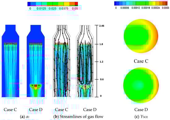
Figure 15.
The figure displays (a) the liquid volume fraction, (b) streamlines of gas flow, and (c) the mass fraction of SO2 from the top view at y = 0.615 m for Case C (empty tower) and Case D (one-tray tower).
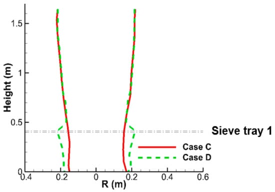
Figure 16.
This schematic shows the radius of liquid column of the small-scale tower for Case C and D.
Correspondingly, the high SO2 region near the wall of tower is reduced significantly from Case C to Case D, as shown in Figure 15c at y = 0.615 m. The stronger two-phase mixing near the sieve tray and smaller region of high SO2 near the wall lead to a higher SO2 removal efficiency for Case D (61.6%) than Case C (56.9%) in Table 6. In comparison with the four-tray Case A in Figure 13, the one-tray Case D in Figure 15c reduces the high SO2 region significantly, while it lacks two-phase mixing from the other three trays. The benefit of the first overwhelms the drawback from the latter, which makes Case D with only one tray perform better than Case A (57.1%).
4.3. Comparisons between Different Inlet Gas Flow Rates (Case E–Case G)
From Case A to Case D, the inlet gas volume flow rates Q are all 24 m3/min, as shown in Table 6. Further increase in gas volume flow rates to 36 m3/min are applied at empty, one-tray, and four-tray tower as Case E, Case F, and Case G. The two-phase inertial loss coefficients are set up as Cg,y = 15.7 (33% increase from Equation (16)) and Cl,y = 10.31 under the same treatments as described in Section 3.5.
The stronger inertia of gas flow deflects the liquid flow into the right side of the tower for Case E (empty tower), as shown in Figure 17a, and its streamlines of gas phase in Figure 17b indicate that the two-phase mixing is very weak in the left of the tower because of the deflection. Therefore, its SO2 removal efficiency is only 48% in Table 6. As for Case F in Figure 17a, the sieve tray can enhance the uniformity of the gas flow [4] to avoid the deflection in the empty tower and exhibit a better two-phase mixing, as shown in Figure 17b. As a result, the SO2 removal efficiency increases from 48% to 58.9%, as shown in Table 6.
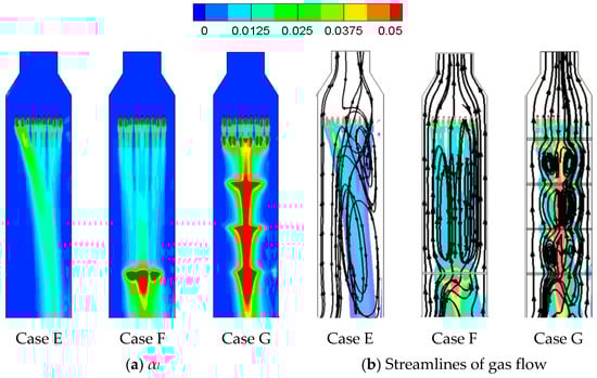
Figure 17.
The figure displays (a) the liquid volume fraction and (b) streamlines of gas flow for Case E–Case G.
With a lower Q of 24 m3/min, the implementation of an additional three sieve trays reduces the SO2 removal efficiency from 61.6% (Case D) to 57.1% (Case A), as discussed in Section 4.2 and shown in Table 6. With all four sieve trays implemented, the gas and liquid flow structures of Case G in Figure 17 are very similar to those of Case A in Figure 12 under a lower value of Q. However, the full implementation of sieve tray under a higher Q of 36 m3/min enhances the efficiency from 58.8% (Case F) to 63% (Case G) and even increases the efficiency by 15% from the empty tower (Case E).
As the inertia of the uprising gas flow is stronger as Q increases, the acceleration of downward liquid flow as that discussed in Figure 8 for Case A becomes weaker. For Case A with Q = 24 m3/min, the downward liquid flow velocity can reach maximum velocity of 2.5 m/s between two trays, while it is only 1.9 m/s for Case G. This weaker acceleration leads to a gentler reduction of the size of liquid column. As a result, the radius of liquid column for four-tray Case G is only 26% smaller than that of one-tray Case F, as illustrated in Figure 18 (Q = 36 m3/min), while the additional three sieve trays incur a greater reduction of 48% (from Case A to Case D), as shown in Figure 14 and Figure 16 (Q = 24 m3/min).
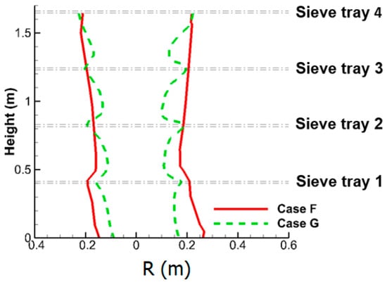
Figure 18.
This schematic shows the radius of liquid column of the small-scale tower for Cases F and G.
Correspondingly, in comparisons with Case F, the full implementation of sieve tray for Case G significantly enhances the two-phase mixing between neighboring trays in Figure 17b, and only reduces the size of liquid column by 26% in Figure 18. The former suppresses the latter and favors the SO2 removal efficiency, as shown in Table 6 for Q = 36 m3/min.
5. Conclusions
This study applied an Eulerian–Eulerian two-phase model with Navier–Stokes equations, porous media model, standard k-ε turbulence closure, and species equations to investigate the fluid mechanics and desulfurization process within the FGD tower of sieve trays. Important findings and contributions can be highlighted as follows:
- The complex structures of sieve trays are replaced by the porous media model, which significantly saves the computational time with consistent results with those simulated by detailed perforated structures and measured data in a small-scale FGD tower. As for the full-scale tower, the computational cost with detailed structure is too expansive considering the enormous scale ratio between the perforated hole at the sieve tray and radius of tower. The porous media model makes the simulations of full-scale tower more practical and was validated in the experiments, which further proves the feasibility of using a porous media model.
- The liquid column from the nozzle experiences deceleration near the top surface of sieve tray and acceleration within it. As the liquid flow has not reached its terminal velocity, the acceleration remains even the liquid passes the tray region. The deceleration leads to the accumulation of liquid volume fraction near the sieve tray, while the acceleration reduces the size of liquid column because of continuity. These mechanisms result in the reduction of liquid column between two neighboring sieve trays and affect the two-phase mixing within the FGD tower.
- The empty, one-tray, and four-tray towers were simulated at different flow conditions. The size of liquid column with better two-phase mixing in the center and the area of uprising gas near the wall play the most important roles to determine the desulfurization performance. At different flow conditions, such as the variation of inlet gas flow rate, these two competing effects end up with different results, which also affects the selections of tray setups.
- The four-tray tower has the best two-phase mixing. However, its liquid column is the smallest, which also ensues the largest area of uprising gas near the wall with higher SO2 concentration. As a result, the four-tray tower at a lower gas flow rate fails to improve the SO2 removal efficiency from the other two tray setups at a lower gas flow rate.
- For a higher inlet gas volume flow rate, the stronger inertial of uprising gas flow leads to a weaker acceleration of the liquid column, and hence, the reduction in size of the liquid column is gentler. Correspondingly, implementing four sieve trays is more efficient under a higher gas volume flow rate. It enhances the performance by 15% from empty tower and 5% from one-tray tower.
- Section 4.2 and Section 4.3 indicate that the sieve tray can enhance two-phase mixing within the liquid column, but it also increases the region of uprising gas where the SO2 mass fraction is higher. Depending on different values of the gas volume flow rate Q, these two competing effects end up with different trends for SO2 removal efficiency.
Author Contributions
Conceptualization, C.-C.T.; methodology, C.-C.T.; software, C.-J.L.; validation, C.-C.T. and C.-J.L.; formal analysis, C.-C.T.; investigation, C.-C.T. and C.-J.L.; resources, C.-C.T.; data curation, C.-C.T.; writing—original draft preparation, C.-C.T.; writing—review and editing, C.-C.T.; visualization, C.-J.L.; supervision, C.-C.T.; project administration, C.-C.T.; funding acquisition, C.-C.T. All authors have read and agreed to the published version of the manuscript.
Funding
This research was funded by MOST under Grant No. MOST 110-2628-E-006-002–and China Steel Cooperation under Grant No. 03A210393.
Institutional Review Board Statement
Not applicable.
Informed Consent Statement
Not applicable.
Data Availability Statement
The data presented in this study are available upon request from the corresponding author.
Acknowledgments
Special thanks Sheng-Yen Hsu in National Sun Yat-sen university for their help, and thanks China Steel Cooperation and China Ecotek Cooperation for their experimental. Additionally, thanks for the funding support of MOST under Grant No. MOST 110-2628-E-006-002-.
Conflicts of Interest
The authors declare no conflict of interest.
Nomenclatures
| Symbol | |
| Aint | Interfacial contact area per unit volume |
| Cqp | Molar concentration of species p in q phase |
| Cq,i | Inertial loss coefficient of phase q in i direction |
| Cd | Drag coefficient |
| Dh | Hole diameter |
| dl | Liquid droplet diameters |
| ESO2 | Enhancement factor for SO2 |
| f | Drag function |
| fh | Porosity |
| G | Gravity |
| HSO2 | Henry’s law constant for SO2 |
| Ki | Exchange coefficient in momentum equations |
| K1,K2,K3 | Equilibrium constants |
| KgSO2, KlSO2 | Mass transfer coefficients for SO2 in the gas and liquid phases |
| k | Turbulence kinetic energy |
| M | Momentum sink term for porous media model |
| P | Pressure |
| Reh | Hole Reynolds number |
| Rer | Relative Reynolds number |
| S | Chemical source term |
| t | Time |
| th | Thickness of the porous media region |
| u | Velocity |
| W | Molecular weight |
| xi | i direction |
| Y | Mass fraction |
| Greek symbols | |
| α | Volume fraction |
| τ | Laminar stress |
| τR | Reynolds stress |
| τr | Relaxation time |
| μ | Mixture viscosity |
| ε | Turbulent dissipation rate |
| ρ | Density |
| ξ1, ξ2, ξ3, ξ4, λ | Tabulated coefficients for the porous media model |
| Subscripts | |
| g | gas phase |
| i, j | Direction |
| l | liquid phase |
| M | Mg(OH)2 solution |
| Slurry | Liquid slurry |
References
- Gao, X.; Huo, W.; Luo, Z.-Y.; Cen, K.-F. CFD simulation with enhancement factor of sulfur dioxide absorption in the spray scrubber. J. Zhejiang Univ. A 2008, 9, 1601–1613. [Google Scholar] [CrossRef]
- Nygaard, H.G.; Kiil, S.; Johnsson, J.E.; Jensen, J.N.; Hansen, J.; Fogh, F.; Dam-Johansen, K. Full-scale measurements of SO2 gas phase concentrations and slurry compositions in a wet flue gas desulphurisation spray absorber. Fuel 2004, 83, 1151–1164. [Google Scholar] [CrossRef]
- Sai, J.; Wu, S.; Xu, R.; Sun, R.; Zhao, Y.; Qin, Y. Mass transfer and reaction process of the wet desulfurization reactor with falling film by cross-flow scrubbing. Korean J. Chem. Eng. 2007, 24, 481–488. [Google Scholar] [CrossRef]
- Tseng, C.-C.; Li, C.-J. Numerical investigation of the inertial loss coefficient and the porous media model for the flow through the perforated sieve tray. Chem. Eng. Res. Des. 2016, 106, 126–140. [Google Scholar] [CrossRef]
- Tseng, C.-C.; Li, C.-J. Eulerian-Eulerian numerical simulation for a flue gas desulfurization tower with perforated sieve trays. Int. J. Heat Mass Transf. 2018, 116, 329–345. [Google Scholar] [CrossRef]
- Brogren, C.; Hakansson, R.; Benton, K.; Rader, P. Performance enhancement plates (PEP): Up to 20 percent reduction in power consumption of wfgd. In Proceedings of the Combined power plant pollutant control mega symposium, Atlanta, GA, USA, 16–20 August 1999. [Google Scholar]
- Dopatka, J.; Ford, N.; Jiajanpong, K. Opportunities to achieve improved WFGD performance and economics. In Proceedings of the Combined Power Plant Control Mega Symposium 2003, Washington, DC, USA, 19–22 May 2003. [Google Scholar]
- Zhu, J.; Zhao, P.; Yang, S.; Chen, L.; Zhang, Q.; Yan, Q. Continuous SO2 absorption and desorption in regenerable flue gas desulfurization with ethylenediamine-phosphoric acid solution: A rate-based dynamic modeling. Fuel 2021, 292, 120263. [Google Scholar] [CrossRef]
- Marocco, L.; Inzoli, F. Multiphase Euler–Lagrange CFD simulation applied to wet flue gas desulphurisation technology. Int. J. Multiph. Flow 2009, 35, 185–194. [Google Scholar] [CrossRef]
- Gómez, A.; Fueyo, N.; Tomás, A. Detailed modelling of a flue-gas desulfurisation plant. Comput. Chem. Eng. 2007, 31, 1419–1431. [Google Scholar] [CrossRef]
- Qu, J.; Qi, N.; Li, Z.; Zhang, K.; Wang, P.; Li, L. Mass transfer process intensification for SO2 absorption in a commercial-scale wet flue gas desulfurization scrubber. Chem. Eng. Process. Process Intensif. 2021, 166, 108478. [Google Scholar] [CrossRef]
- Qu, J.; Qi, N.; Zhang, K.; Li, L.; Wang, P. Wet flue gas desulfurization performance of 330 MW coal-fired power unit based on computational fluid dynamics region identification of flow pattern and transfer process. Chin. J. Chem. Eng. 2021, 29, 13–26. [Google Scholar] [CrossRef]
- Xu, Y.; Chen, X.; Zhao, Y.; Jin, B. Modeling and analysis of CO2 capture by aqueous ammonia + piperazine blended solution in a spray column. Sep. Purif. Technol. 2021, 267, 118655. [Google Scholar] [CrossRef]
- Deng, Q.; Ran, J.; Niu, J.; Yang, Z.; Pu, G.; Yang, L. Numerical Study on Flow Field Distribution Regularities in Wet Gas Desulfurization Tower Changing Inlet Gas/Liquid Feature Parameters. J. Energy Resour. Technol. 2020, 143, 023005. [Google Scholar] [CrossRef]
- Du, J.; Hui, Z.; Wu, F.; Yan, Y.; Yue, K.; Ma, X. CFD Analysis of a Water Vaporization Process in a Three-Dimensional Spouted Bed for Flue Gas Desulfurization. ACS Omega 2021, 6, 2759–2766. [Google Scholar] [CrossRef] [PubMed]
- Wu, F.; Bai, J.; Yue, K.; Gong, M.; Ma, X.; Zhou, W. Eulerian-Eulerian Numerical Study of the Flue Gas Desulfurization Process in a Semidry Spouted Bed Reactor. ACS Omega 2020, 5, 3282–3293. [Google Scholar] [CrossRef]
- Jamshidifard, S.; Shirvani, M.; Kasiri, N.; Movahedirad, S. Fine particle removal from gas stream using a helical-duct dust concentrator: Numerical study. Chem. Eng. Process. Process Intensif. 2019, 143, 107516. [Google Scholar] [CrossRef]
- Chou, Y.-J.; Shao, Y.-C. Numerical study of particle-induced Rayleigh-Taylor instability: Effects of particle settling and entrainment. Phys. Fluids 2016, 28, 043302. [Google Scholar] [CrossRef]
- Sun, Y.; Guan, Z.; Gurgenci, H.; Hooman, K.; Li, X.; Xia, L. Investigation on the influence of injection direction on the spray cooling performance in natural draft dry cooling tower. Int. J. Heat Mass Transf. 2017, 110, 113–131. [Google Scholar] [CrossRef]
- Crowe, C.T.; Sharma, M.P.; Stock, D.E. The Particle-Source-In Cell (PSI-CELL) Model for Gas-Droplet Flows. J. Fluids Eng. 1977, 99, 325–332. [Google Scholar] [CrossRef]
- Benyahia, S.; Galvin, J.E. Estimation of numerical errors related to some basic assumptions in discrete particle methods. Ind. Eng. Chem. Res. 2010, 49, 10588–10605. [Google Scholar] [CrossRef] [Green Version]
- ANSYS Fluent. ANSYS Fluent 12.0 User’s Guide; Ansys Inc.: Canonsburg, PA, USA, 2009; Volume 15317, pp. 1–2498. [Google Scholar]
- Choi, M.; Lim, Y.; Lee, H.; Jung, H.; Lee, J. Flow uniformizing distribution panel design based on a non-uniform porosity distribution. J. Wind Eng. Ind. Aerodyn. 2014, 130, 41–47. [Google Scholar] [CrossRef]
- Chen, Z.; Wang, H.; Zhuo, J.; You, C. Experimental and numerical study on effects of deflectors on flow field distribution and desulfurization efficiency in spray towers. Fuel Process. Technol. 2017, 162, 1–12. [Google Scholar] [CrossRef]
- Guo, B.; Hou, Q.; Yu, A.; Li, L.; Guo, J. Numerical modelling of the gas flow through perforated plates. Chem. Eng. Res. Des. 2013, 91, 403–408. [Google Scholar] [CrossRef]
- Ergun, S. Fluid flow through packed columns. Chem. Eng. Prog. 1952, 48, 89–94. [Google Scholar]
- Jackson, G.W.; James, D.F. The permeability of fibrous porous media. Can. J. Chem. Eng. 1986, 64, 364–374. [Google Scholar] [CrossRef]
- Idelchik, I.E. Handbook of Hydraulic Resistance, 3rd ed.; Begell Houss: Danbury, CT, USA, 1996. [Google Scholar]
- Wenbin, L.; Botan, L.; Guocong, Y.; Xigang, Y. A new model for the simulation of distillation column. Chin. J. Chem. Eng. 2011, 19, 717–725. [Google Scholar]
- Shyy, W.; Thakur, S.S.; Ouyang, H.; Liu, J.; Blosch, E. Computational Techniques for Complex Transport Phenomena; Cambridge University Press: Cambridge, UK, 1997. [Google Scholar]
- Launder, B.; Spalding, D. The numerical computation of turbulent flows. Comput. Methods Appl. Mech. Eng. 1974, 3, 269–289. [Google Scholar] [CrossRef]
- Schiller, L.; Naumann, A. A drag coefficient correlation. Zeit. Ver. Deutsch. Ing. 1933, 77, 318–320. [Google Scholar]
- Harris, D.C. Quantitative Chemical Analysis; Macmillan: New York, NY, USA, 2010. [Google Scholar]
- China Steel Cooperation. 2021. Available online: http://www.csmc.com.tw/csr06_ch.aspx (accessed on 31 December 2021).
- Patankar, S.V. Numerical Heat Transfer and Fluid Flow; Hemisphere: Washington, DC, USA, 1980. [Google Scholar]
- Huang, Y.S.; Tseng, C.C.; Chien, C.C. Numerical Simulation of the Flue Gas Desulfurization in the Sieve Tray Tower. China Steel Rep. 2015, 28, 52–57. [Google Scholar]
Publisher’s Note: MDPI stays neutral with regard to jurisdictional claims in published maps and institutional affiliations. |
© 2022 by the authors. Licensee MDPI, Basel, Switzerland. This article is an open access article distributed under the terms and conditions of the Creative Commons Attribution (CC BY) license (https://creativecommons.org/licenses/by/4.0/).