
Analytical Design of Fractional-Order PI Controller for Parallel Cascade Control Systems

Abstract
:1. Introduction
2. Materials and Methods
2.1. Fractional Calculus
2.2. Crone Approximation
2.3. Fractional Linear Model
2.4. The FOPI Controller in the Frequency Domain
2.5. Maximum Sensitivity Value
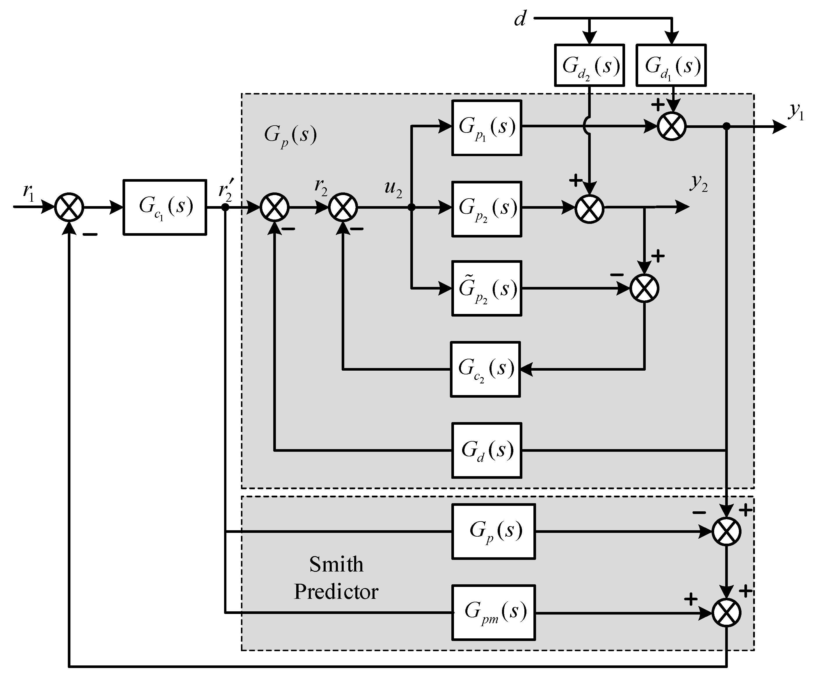
2.6. Analytical Design of FOPI Controller for PCCS Combining with Smith Predictor
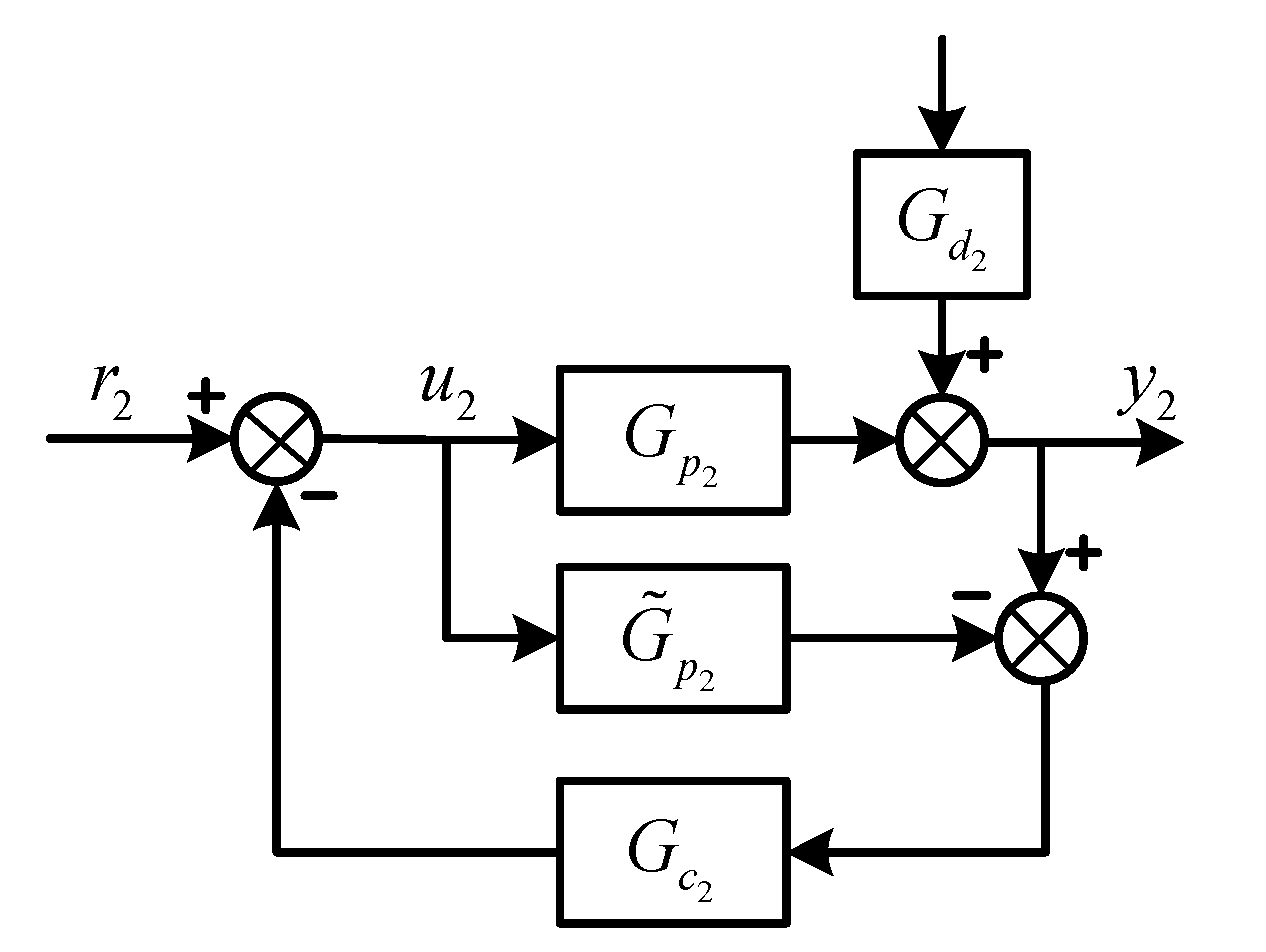
2.6.1. Design of Secondary Controller Based on IMC Approach for Disturbance Rejection
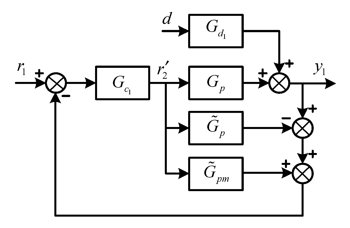
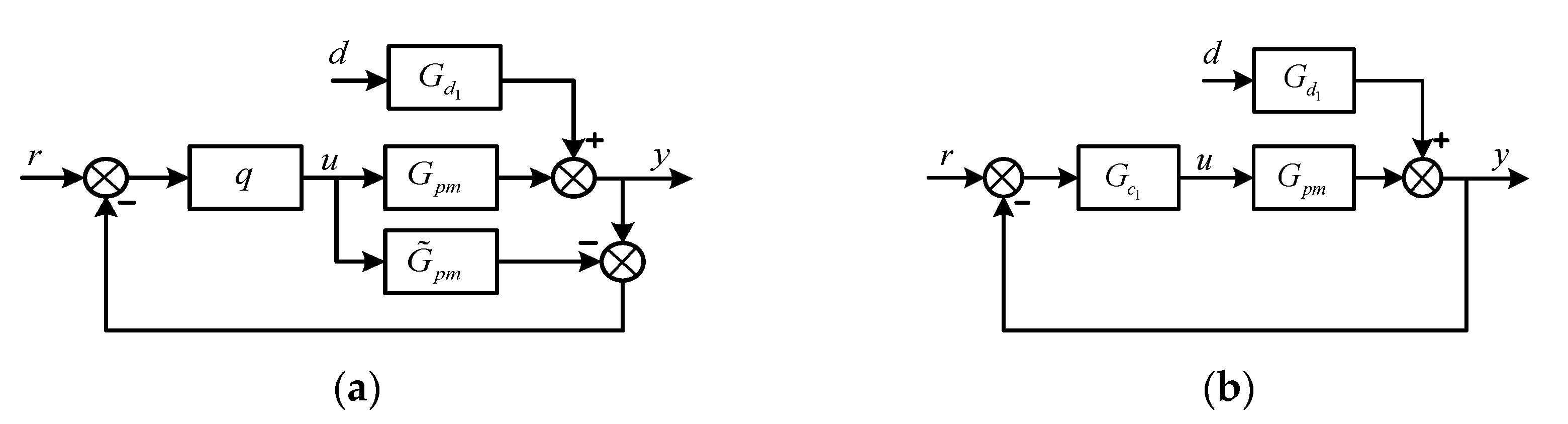
2.6.2. FOPI Controller Design for the Primary Control Loop
2.6.3. The General Proposed Design Method for the Above Three Cases of the Primary Controller
| Algorithm 1: The proposed tuning algorithm for case 2. |
| 1: Initialization |
| Calculate according to Equations (32) and (41) ; ; assign the value of |
| do |
| according to Equation (31) |
| based on Equation (40) |
| according to Equations (50) and (51) |
| for each set of control parameters |
| by: |
| : assign % avoid an infinite loop |
| 9: end while |
| 10: end |
| Algorithm 2: The proposed tuning algorithm for case 3. |
| 1: Initialization |
| Calculate according to Equations (36) and (37) Choose from this range |
| according to Equation (35) |
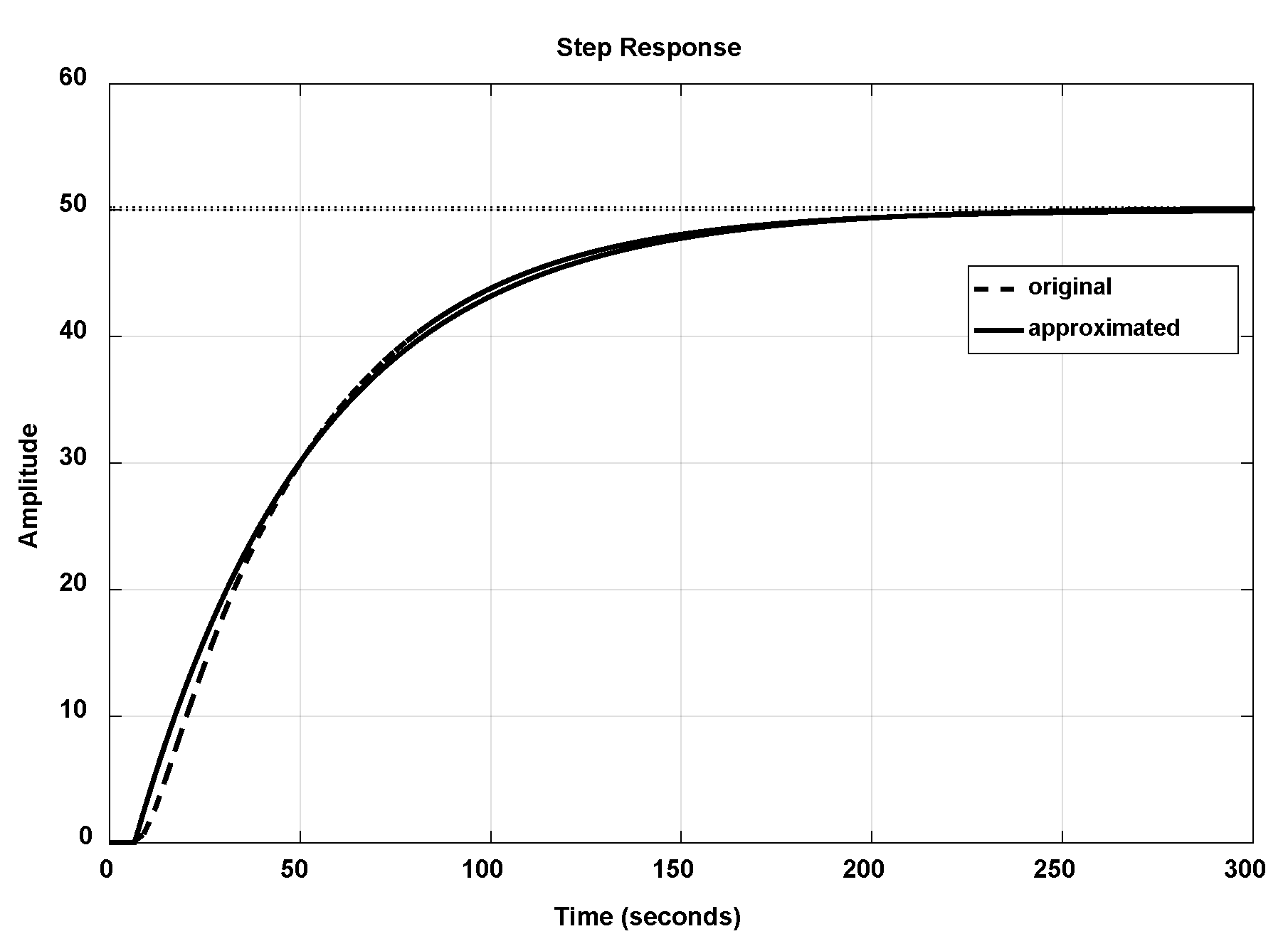
| 3: Approximate into FOPDT using PSO algorithm |
| based on Equation (40) |
| according to Equations (50) and (51) |
| 6: end |
3. Results
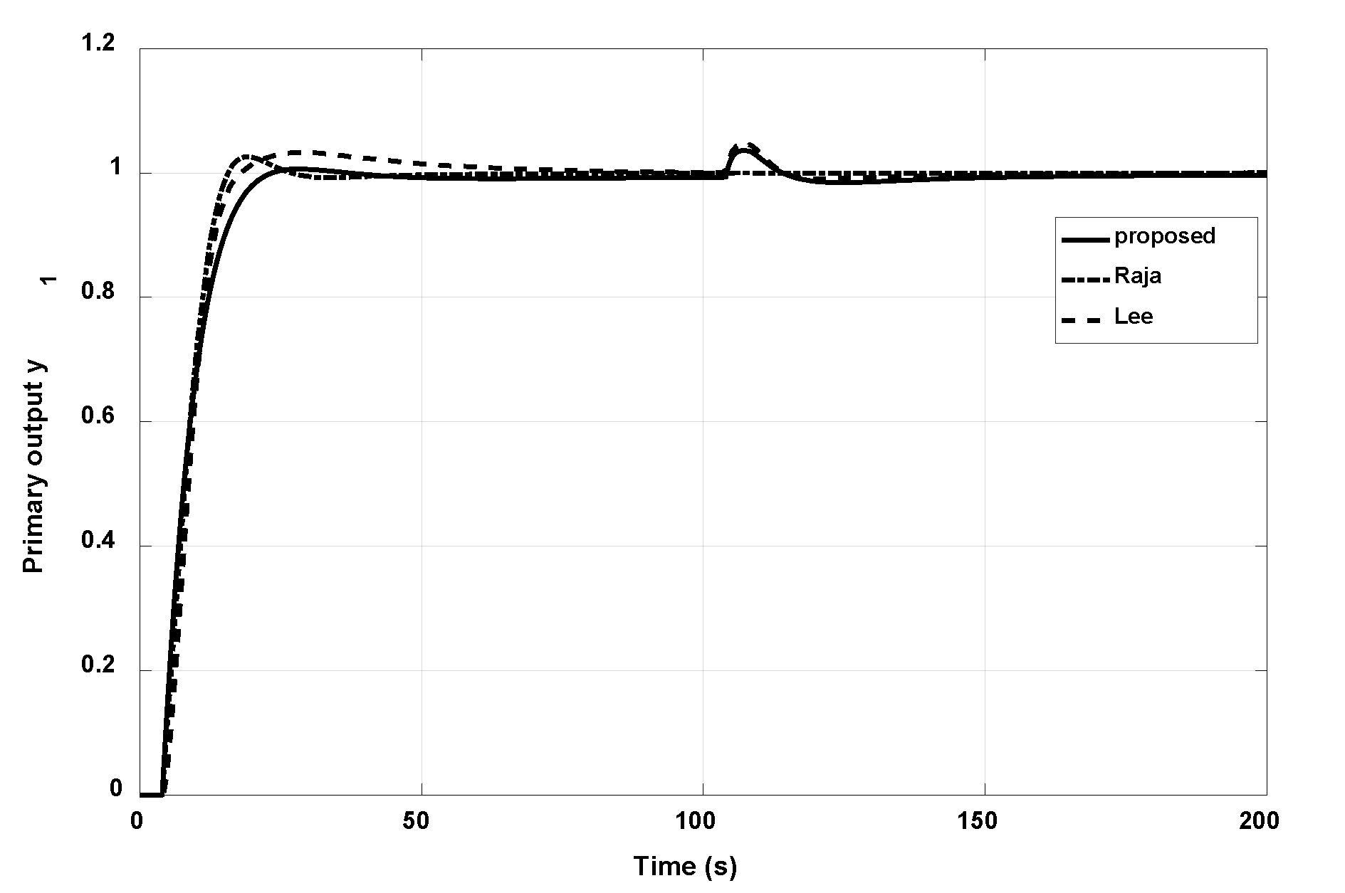
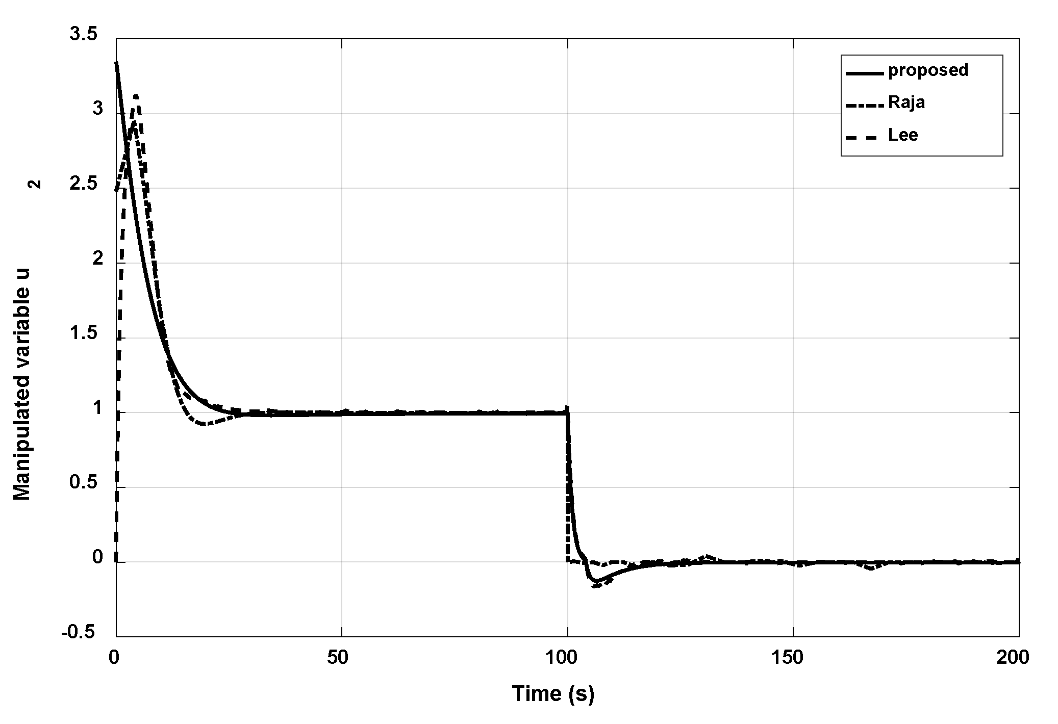
3.1. Example 1
- -
- Step 1: Determine the stabilized controller, in this example . Therefore, the equivalent transfer function of the primary loop is derived as in Equation (54):
- -
- Step 2: Applying Equations (40), (50), and (51) to derive the control parameters. The obtained controller and is shown in Table 1.
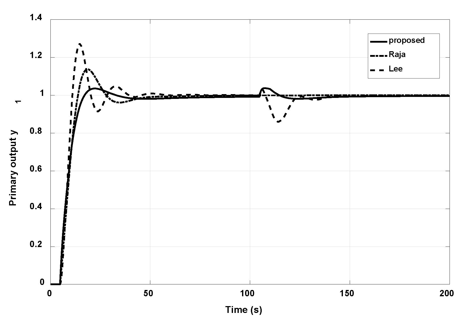
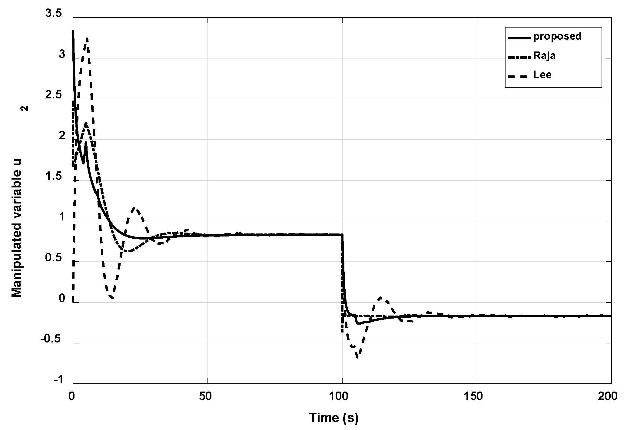
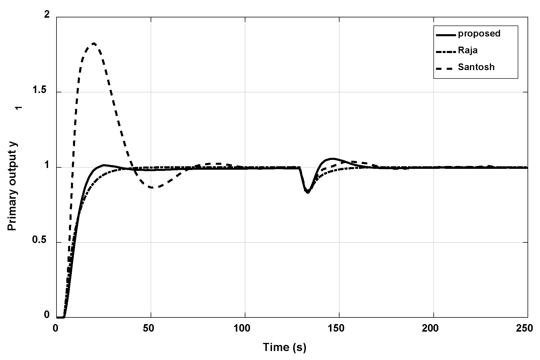
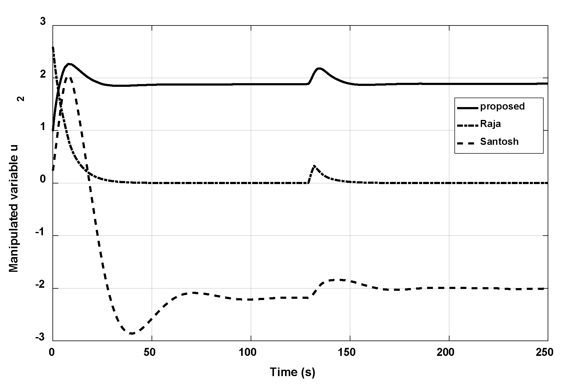
3.2. Example 2
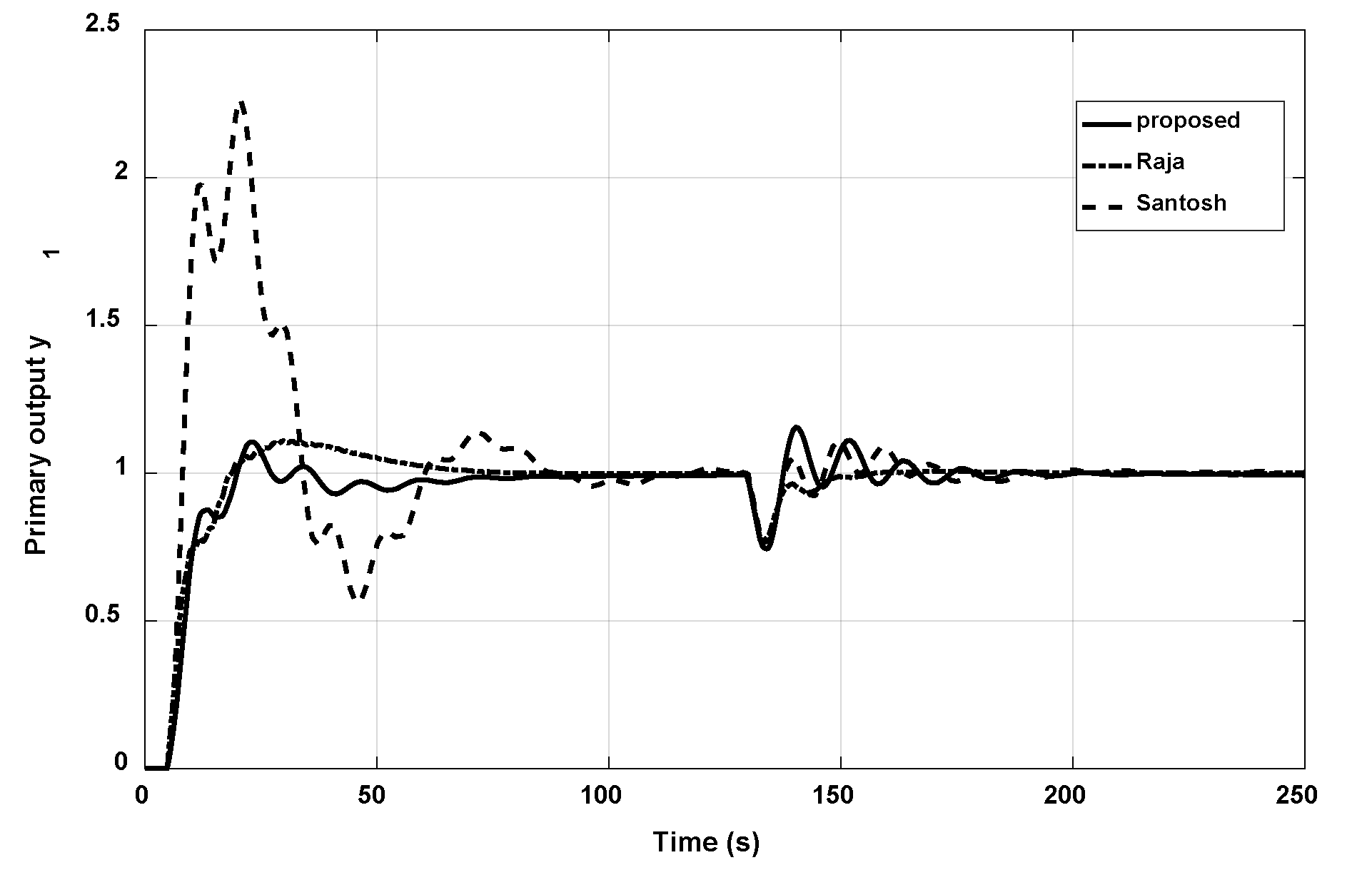
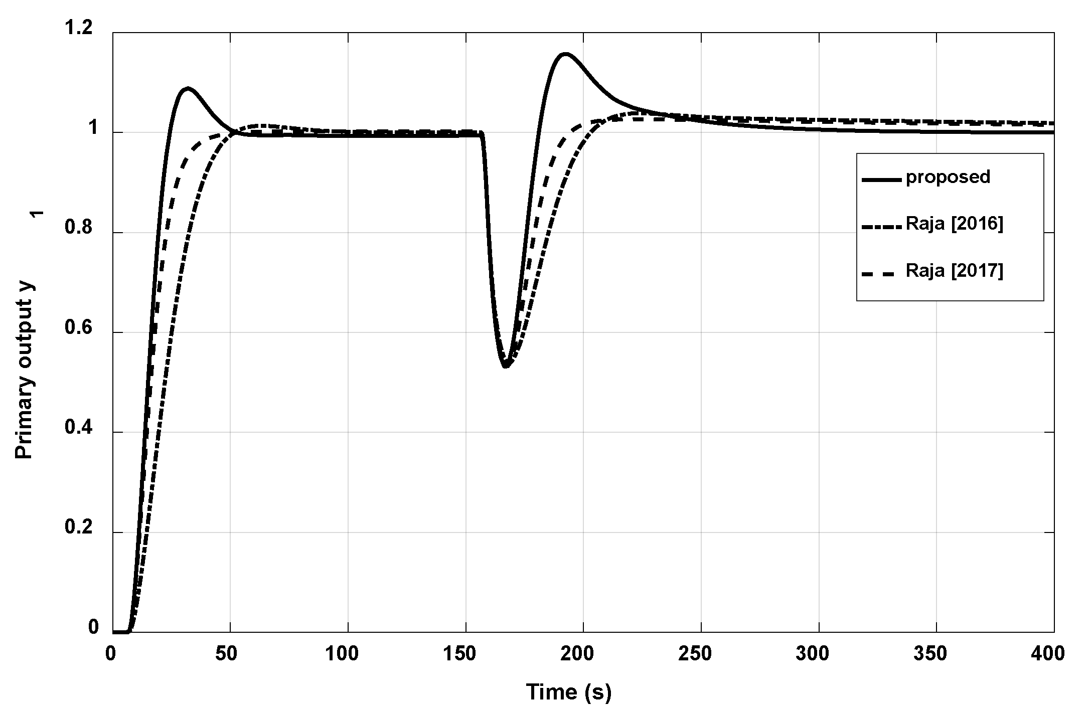
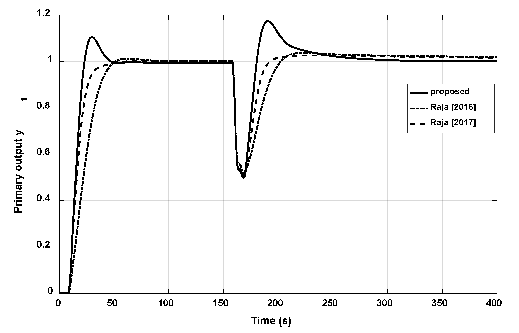
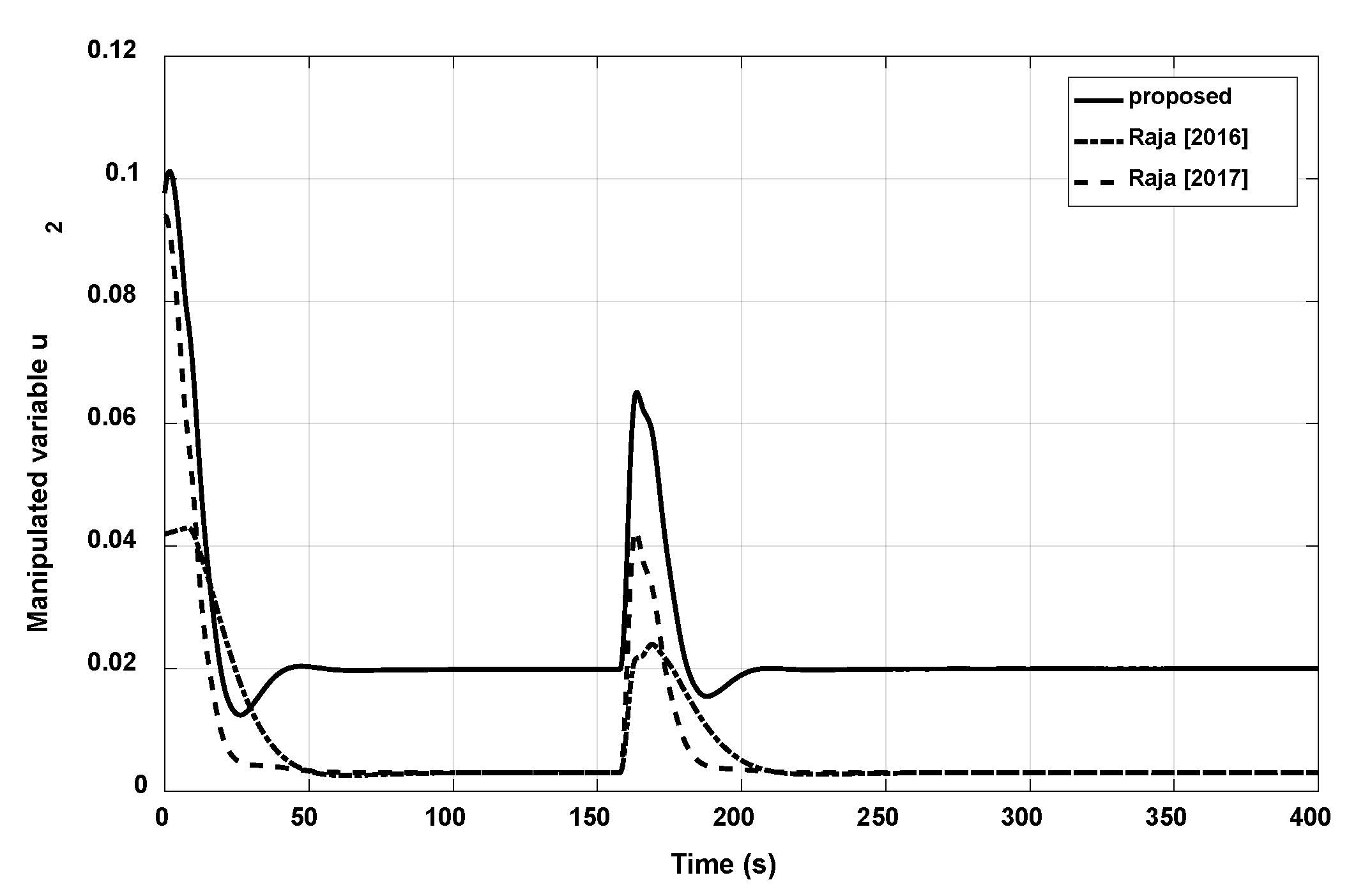
3.3. Example 3
4. Conclusions
Author Contributions
Funding
Institutional Review Board Statement
Informed Consent Statement
Data Availability Statement
Conflicts of Interest
References
- Luyben, W.L. Parallel Cascade Control. Ind. Eng. Chem. Fundam. 1973, 12, 463–467. [Google Scholar] [CrossRef]
- Santosh, S.; Chidambaram, M. A simple method of tuning parallel cascade controllers for unstable FOPTD systems. ISA Trans. 2016, 65, 475–486. [Google Scholar] [CrossRef] [PubMed]
- Raja, G.L.; Ali, A. Modified parallel cascade control strategy for stable, unstable and integrating processes. ISA Trans. 2016, 65, 394–406. [Google Scholar] [CrossRef] [PubMed]
- Lee, Y.; Skliar, M.; Lee, M. Analytical method of PID controller design for parallel cascade control. J. Process Control 2006, 16, 809–818. [Google Scholar] [CrossRef]
- Rao, A.S.; Seethaladevi, S.; Uma, S.; Chidambaram, M. Enhancing the performance of parallel cascade control using Smith predictor. ISA Trans. 2009, 48, 220–227. [Google Scholar]
- Uma, S.; Chidambaram, M.; Rao, A.S.; Yoo, C.K. Enhanced control of integrating cascade processes with time delays using modified Smith predictor. Chem. Eng. Sci. 2010, 65, 1065–1075. [Google Scholar] [CrossRef]
- Padhan, D.G.; Majhi, S. An improved parallel cascade control structure for processes with time delay. J. Process Control 2012, 22, 884–898. [Google Scholar] [CrossRef]
- Raja, G.L.; Ali, A. Smith predictor based parallel cascade control strategy for unstable and integrating processes with large time delay. J. Process Control 2017, 52, 57–65. [Google Scholar] [CrossRef]
- Pashaei, S.; Bagheri, P. Parallel cascade control of dead time processes via fractional order controllers based on Smith predictor. ISA Trans. 2020, 98, 186–197. [Google Scholar] [CrossRef]
- Monje, C.A.; Chen, Y.Q.; Vinagre, B.M.; Xue, D.Y.; Feliu, V. Fractional-Order Systems and Controls, Fundamentals and Applications; Springer: London, UK, 2010. [Google Scholar]
- Bucolo, M.; Buscarino, A.; Famoso, C.; Fortuna, L.; Gagliano, S. Imperfections in Integrated Devices Allow the Emergence of Unexpected Strange Attractors in Electronic Circuits. IEEE Access 2021, 9, 29573–29583. [Google Scholar] [CrossRef]
- Caponetto, R.; Dongola, G.; Fortuna, L.; Petráš, I. Fractional Order Systems: Modeling and Control Applications; World Scientific: Singapore, 2010; Volume 72. [Google Scholar]
- Podlubny, I. Fractional-Order Systems and PIλDμ-Controllers. IEEE Trans. Autom. Control 1999, 44, 208–214. [Google Scholar] [CrossRef]
- Chen, Y.Q.; Bhaskaran, T.; Xue, D.Y. Practical Tuning Rule Development for Fractional Order Proportional and Integral Controllers. J. Comput. Nonlinear Dyn. 2008, 3, 021403. [Google Scholar] [CrossRef] [Green Version]
- Luo, Y.; Chen, Y.Q.; Wang, C.Y.; Pi, Y.G. Tuning fractional order proportional integral controllers for fractional order systems. J. Process Control 2010, 20, 823–831. [Google Scholar] [CrossRef]
- Padula, F.; Visioli, A. Tuning rules for optimal PID and fractional-order PID controllers. J. Process Control 2011, 21, 69–81. [Google Scholar] [CrossRef]
- Li, M.; Zhou, P.; Zhao, Z.; Zhang, J. Two-degree-of-freedom fractional order-PID controllers design for fractional order processes with dead-time. ISA Trans. 2016, 61, 147–154. [Google Scholar] [CrossRef] [Green Version]
- Vu, T.N.L.; Lee, M. Analytical design of fractional-order proportional-integral controllers for time-delay processes. ISA Trans. 2013, 52, 583–591. [Google Scholar] [CrossRef]
- Beschi, M.; Padula, F.; Visioli, A. Fractional robust PID control of a solar furnace. Control Eng. Pract. 2016, 60, 190–199. [Google Scholar] [CrossRef]
- Li, D.; Liu, L.; Jin, Q.; Hirasawa, K. Maximum sensitivity based fractional IMC-PID controller design for non-integer order system with time delay. J. Process Control 2015, 31, 17–29. [Google Scholar] [CrossRef]
- Vilanova, R.; Arrieta, O.; Ponsa, P. Robust PI/PID controllers for load disturbance based on direct synthesis. ISA Trans. 2018, 81, 177–196. [Google Scholar] [CrossRef]
- Yumuk, E.; Guzelkaya, M.; Eksin, I. Analytical fractional PID controller design based on Bode’s ideal transfer function plus time delay. ISA Trans. 2019, 91, 196–206. [Google Scholar] [CrossRef]
- Moradi, M. A genetic-multivariable fractional order PID control to multi-input multi-output processes. J. Process Control 2014, 24, 336–343. [Google Scholar] [CrossRef]
- Sánchez, H.S.; Padula, F.; Visioli, A.; Vilanova, R. Tuning rules for robust FOPID controllers based on multi-objective optimization with FOPDT models. ISA Trans. 2017, 66, 344–361. [Google Scholar] [CrossRef] [Green Version]
- Hajiloo, A.; Nariman-Zadeh, N.; Moeini, A. Pareto optimal robust design of fractional-order PID controllers for systems with probabilistic uncertainties. Mechatronics 2012, 22, 788–801. [Google Scholar] [CrossRef]
- Pan, I.; Das, S. Chaotic multi-objective optimization-based design of fractional order PIλDµ controller in AVR system. Electr. Power Energy Syst. 2012, 43, 393–407. [Google Scholar] [CrossRef] [Green Version]
- Morari, M.; Zafiriou, E. Robust Process Control, Englewood Cliffs; Prentice Hall: Hoboken, NJ, USA, 1989. [Google Scholar]
- Skogestad, S.; Postlethwaithe, I. Multivariable Feedback Control Analysis and Design, 1st ed.; John Wiley & Sons: Hoboken, NJ, USA, 1996. [Google Scholar]
- Chuong, V.L.; Vu, T.N.L.; Truong, N.T.N.; Jung, J.H. An Analytical Design of Simplified Decoupling Smith Predictors for Multivariable Processes. Appl. Sci. 2019, 9, 2487. [Google Scholar] [CrossRef] [Green Version]


| Secondary Loop | Primary Loop | ||
|---|---|---|---|
| Proposed | |||
| Raja | |||
| Lee (Case B) | |||
| Nominal | Perturbed (±20%) | |||||
|---|---|---|---|---|---|---|
| IAE | ISE | TV | IAE | ISE | TV | |
| Proposed | 6.1723 | 2.7231 | 3.6211 | 6.6548 | 2.8601 | 4.3013 |
| Raja | 8.8062 | 6.8088 | 4.0936 | 10.8054 | 7.6263 | 4.7519 |
| Lee (case B) | 10.727 | 7.4696 | 7.9901 | 12.3538 | 7.8052 | 12.430 |
| Secondary Loop | Primary Loop | ||
|---|---|---|---|
| Proposed | |||
| Raja | |||
| Santosh | |||
| Nominal | Perturbed (±20%) | |||||
|---|---|---|---|---|---|---|
| IAE | ISE | TV | IAE | ISE | TV | |
| Proposed | 8.9633 | 4.0985 | 2.3717 | 11.1245 | 4.2856 | 4.5196 |
| Raja | 7.9704 | 3.5565 | 3.2496 | 8.9385 | 3.5034 | 4.9707 |
| Santosh | 28.0025 | 16.9457 | 8.2492 | 37.2077 | 24.424 | 11.1628 |
| Secondary Loop | Primary Loop | ||
|---|---|---|---|
| Proposed | |||
| Raja (2016) | |||
| Raja (2017) | |||
| Nominal | Perturbed (±20%) | |||||
|---|---|---|---|---|---|---|
| IAE | ISE | TV | IAE | ISE | TV | |
| Proposed | 17.9520 | 7.5790 | 0.1845 | 18.5801 | 7.9852 | 0.2038 |
| Raja (2016) | 39.9687 | 21.848 | 0.0819 | 39.8605 | 22.166 | 0.0851 |
| Raja (2017) | 17.9977 | 8.1274 | 0.1591 | 17.9531 | 8.3991 | 0.1703 |
Publisher’s Note: MDPI stays neutral with regard to jurisdictional claims in published maps and institutional affiliations. |
© 2022 by the authors. Licensee MDPI, Basel, Switzerland. This article is an open access article distributed under the terms and conditions of the Creative Commons Attribution (CC BY) license (https://creativecommons.org/licenses/by/4.0/).
Share and Cite
Vu, T.N.L.; Chuong, V.L.; Truong, N.T.N.; Jung, J.H. Analytical Design of Fractional-Order PI Controller for Parallel Cascade Control Systems. Appl. Sci. 2022, 12, 2222. https://doi.org/10.3390/app12042222
Vu TNL, Chuong VL, Truong NTN, Jung JH. Analytical Design of Fractional-Order PI Controller for Parallel Cascade Control Systems. Applied Sciences. 2022; 12(4):2222. https://doi.org/10.3390/app12042222
Chicago/Turabian StyleVu, Truong Nguyen Luan, Vo Lam Chuong, Nguyen Tam Nguyen Truong, and Jae Hak Jung. 2022. "Analytical Design of Fractional-Order PI Controller for Parallel Cascade Control Systems" Applied Sciences 12, no. 4: 2222. https://doi.org/10.3390/app12042222
APA StyleVu, T. N. L., Chuong, V. L., Truong, N. T. N., & Jung, J. H. (2022). Analytical Design of Fractional-Order PI Controller for Parallel Cascade Control Systems. Applied Sciences, 12(4), 2222. https://doi.org/10.3390/app12042222