Single and Multiple Continuous-Wave Interference Suppression Using Adaptive IIR Notch Filters Based on Direct-Form Structure in a QPSK Communication System

Abstract

The removal filter coefficients in this technique are dependent on the jammer’s power and its Instantaneous Frequency (IF) information, which can both be obtained in the time–frequency domain (adaptive filtering techniques). The dependence of the removing/reducing filter characteristics on the interference power is critical, as it allows an optimal trade-off between removal interference and the amount of self-noise generated by the filter. This trade-off is bounded by the two extreme cases of no notch filter (no self-noise) and full suppression (k₁ = 1) for both low- and high-power jammer values. In this paper, a cascade second-order adaptive direct Infinite Impulse Response (IIR) Notch Filter (NF) with a gradient-based algorithm to suppress the Continuous-Wave (CW and MCW) interference is proposed for maximizing the receiver Signal-to-Noise Ratio (SNR) in a Quadrature Phase-Shift Keying (QPSK)-modulated signal. The suppression approach consists of two Adaptive IIR NFs (ANFs) based on a direct-form structure: the H_d1(z) and H_d1(z). The proposal in this work presents a low-complexity Time-Domain (TD) algorithm for controlling the update filter coefficient and notch depth. Simulation results demonstrate that the proposed approach represents an effective method for removing/reducing the impacts of CWI/MCWI, resulting in improved system performance for low- and high-power jammer values when compared with the case of full suppression (k₁ = 1); furthermore, it also improves the notch filter’s output SNR for a given Jamming-to-Signal Ratio (JSR) value and Bit Error Ratio (BER) performance. For example, the SNR output of the proposed IIR NF was enhanced by 7 dB versus the case without a filter when E_b/N_o = 15 dB and JSR = −5 dB. The proposed method can detect and mitigate weak and strong jamming with JSR values ranging from −30 to 40 dB, and can track the hopping frequency interference. Moreover, an improved BER performance is seen as compared to the case without an IIR NF.

1. Introduction

As the number of wireless applications in use increases, human-made Radio Frequency Interference (RFI) is continuously increasing. Thus, many communication systems, including wireless communication, suffer from human-made RFI. According to [1,2], interference is any disruption of an electronic system or device caused by external electromagnetic emissions at a Radio Frequency (RF) of interest. Human-made RFI can be classified under either unintentional or intentional acts, such as jamming. RFI affects the receiver, lowers the quality of the Signals-of-Interest (SoI), degrades the communication system’s Quality of Service (QoS), lowers the Signal-to-Noise Ratio (SNR), and increases the BER. Jamming is the deliberate broadcasting of interference signals into the frequency bands of a signal of interest—usually at a higher power than the signal of interest. In the literature, jamming has been studied in a variety of contexts, including Wireless Sensor Networks (WSNs) [3,4], Orthogonal Frequency-Division Multiplexing (OFDM) communications [5], Multi-Hop Wireless Networks (MHWNs) [6], and Long-Term Evolution (LTE) cellular communications [7]. In [8], the authors discuss the negative effects of jamming on GNSS receiver performance, and present three types of jamming detection, namely, digital pre-correlation signal processing, post-correlation domain, and Automatic Gain Control (AGC).

Several techniques have been developed to mitigate the RFIs that impact the receiver in various areas of telecommunications—especially wireless communications. In GNSS signals [9], interference can be easily detected and mitigated, as the distance between the transmitter and the receiver is too large (around 20,000 Km); thus, the signal is Wideband (WB). Additionally, the GNSS signals from the satellites are below the noise level.

Furthermore, a higher Jamming-to-Noise Ratio (JNR) enables easier interference detection [10]. When compared to GNSS signals, the amplitude level of a modulated Narrowband (NB) signal, as defined by the Digital Video Broadcasting Satellite Second Generation (DVB-S2) standard [11,12], is significantly higher than the noise. The modulated NB digital communication signal is the main focus of this work. In the literature, most algorithms used in detection and mitigation techniques are in Wideband (WB) signals that do not work directly with NB signals. Therefore, this work utilizes the Jamming-to-Signal Ratio (JSR) instead of JNR in order to mitigate modulated Narrowband (NB) signals. Figure 1 displays the effect of the Power Spectrum (PS) on the received signal with different JSR parameters, and compares the impact of JSR and the energy per bit to the noise power spectral density ratio ($E_b/N_o$) on the effectiveness of detection. Moreover, Figure 1 also describes multiple CWIs with different JSRs added to the modulated signal (QPSK), where the amplitude of the CWI on top of the original signal is significantly affected by JSR. Figure 2 illustrates the impact of the received PS signal with various $E_b/N_o$ parameters on interference clarity. As can be seen, as $E_b/N_o$ decreases, the noise level increases; however, in comparison with the signal’s power level, this does not affect the location and visibility of the CWI peaks, thus indicating that JSR is the primary effective parameter for interference detection.

Adaptive notch filters (ANFs) were used to eliminate or reduce low and strong RFI impacts. ANF methods can suppress CW and other kinds of NB interference. In a typical IIR NF, a zero is placed on a unit circle with a phase equal to the frequency of the instantaneous jammer, so as to completely remove the jamming However, precisely because the jamming is thus completely eliminated, this method generates a significant amount of self-noise [13], as briefly described in [14]. ANFs, for their part, create self-noise, which significantly reduces the receiver’s SNR in this situation [15]; therefore, the depth of ANFs’ excision NFs is adjusted to JSR specifications. In the case of high-power jammers, a deep notch is required for perfect jamming removal. Many papers have been written on the rejection or mitigation of NB interference using various suppression filters; however, most such works emphasize the suppression of CWI and MCWI, while few studies appear to focus on adjusting the depth of the NF based on an estimation of the power of the interference in suppressing CWI and MCWI.

This paper proposes a technique for suppressing CWI and MCWI based on an adaptive direct IIR NF, focusing on adjusting the depth of the NF. The proposed method overcomes the main drawbacks of ANF while removing interference; it avoids the self-noise effect of the NF by adjusting and controlling the depth of the NF using the ANF $H_{d2}\left(z\right)$.

The main contribution of this work is to propose a new class of adaptive algorithms to control the update filter coefficient and adjust the depth of NFs with respect to estimating the power of interference using a second adaptive IIR NF based on a direct-form structure.

The structure of this paper is as follows: Section 2 reviews previous research. The signal model of the received signal in the presence of interference is described in Section 3. The proposed suppression system model, its adaptation algorithm, and the optimal notch depth are described in Section 4. Section 5 presents the proposed performance based on simulation results, and the paper is concluded in Section 6.

2. Related Works

ANFs have been widely used with mitigation systems in different areas, such as biomedical (e.g., cancel 60 Hz interference) [16,17], communications (e.g., reject NBI in the BPSK spread-spectrum communication system), and GNSS applications [18] and control (e.g., controlling the howling in speakerphone systems) [19]. In the literature, various mitigation techniques already exist to reduce and remove the negative effects of RFIs, which can be classified into three groups: adaptive antenna-based techniques [20], Time–Frequency Filtering (TFF)-based methods [21,22], and adaptive-filtering-based techniques [15,23,24].

Adaptive antenna techniques are useful for WB and NB jammers, but their main disadvantage is their accompanying computational complexity [20,25,26].

TFF-based techniques provide useful information in both the Time Domain (TD) and Frequency Domain (FD) simultaneously [27]. TFFs are mainly used to mitigate NB jamming. Bilinear signal distribution [28], filter banks [29], Short-Time Fourier Transforms (STFTs) [30], and Wavelet Transforms (WTs) [31,32,33] are examples of TFF tools. Filter banks and STFTs cannot simulate most nonstationary signals, due to the use of fixed windows. By adjusting the trade-off between frequency and time, the WT solves the drawbacks of filter banks and STFTs; however, for each type of jamming, it must be tuned to perfection [34].

Adaptive-filtering-based techniques for NB jamming rejection are commonly used, and can be classified into two types: FD and TD. In the FD approach, ref. [35] proposed using automatic gain control (AGC) to mitigate CWI and NB; ref. [36] proposed a method to detect CWI by statistical inference, while [11] proposed an IIR NF for detecting and mitigating MCW by implementing it as a first-order IIR NF and using a simplified Welch algorithm. However, computational complexity and higher costs are the main drawbacks of the FD approach. In the TD approach, the adaptive lattice NF is used to detect and mitigate CWI [18,37]. Moreover, ref. [37] described an ANF method for detecting and reducing MCWI in GPS systems. In GNSS Inter-Satellite Links (ISLs), ref. [38] proposed an adaptive NBI suppression approach based on the code-aided technique; refs. [13,15,39] proposed ANF methods based on a lattice form to mitigate the CWI. A low-complexity method based on a second IIR NF for GNSS to mitigate CWI was proposed in [40]. To reduce and mitigate CWI, ref. [41] presented a new low-complexity anti-jamming NF for general wireless communications, while [42] derived FIR excision filters that optimize receiver SNR for NB interference. In GPS, ref. [42] proposed a method to mitigate CWI using adaptive FIR and ACM filters, while [43] proposed a method based on the lattice-form structure for detecting and mitigating an MCWI by controlling the depth of the NF.

Kalman filters [44], ANFs [15,39,45], Approximate Conditional Mean (ACM) filters [46], neural network-based predictors [44,47], and augmented state ACM (ASACM) filters [48] are examples of adaptive-filtering-based techniques and tools. However, adaptive-filtering-based methods have certain drawbacks. ACM and Kalman filters do not work effectively when a priori knowledge of the jamming model parameters is unavailable. The computational complexity of the ASACM filter increases exponentially in the case of MCWI rejection.

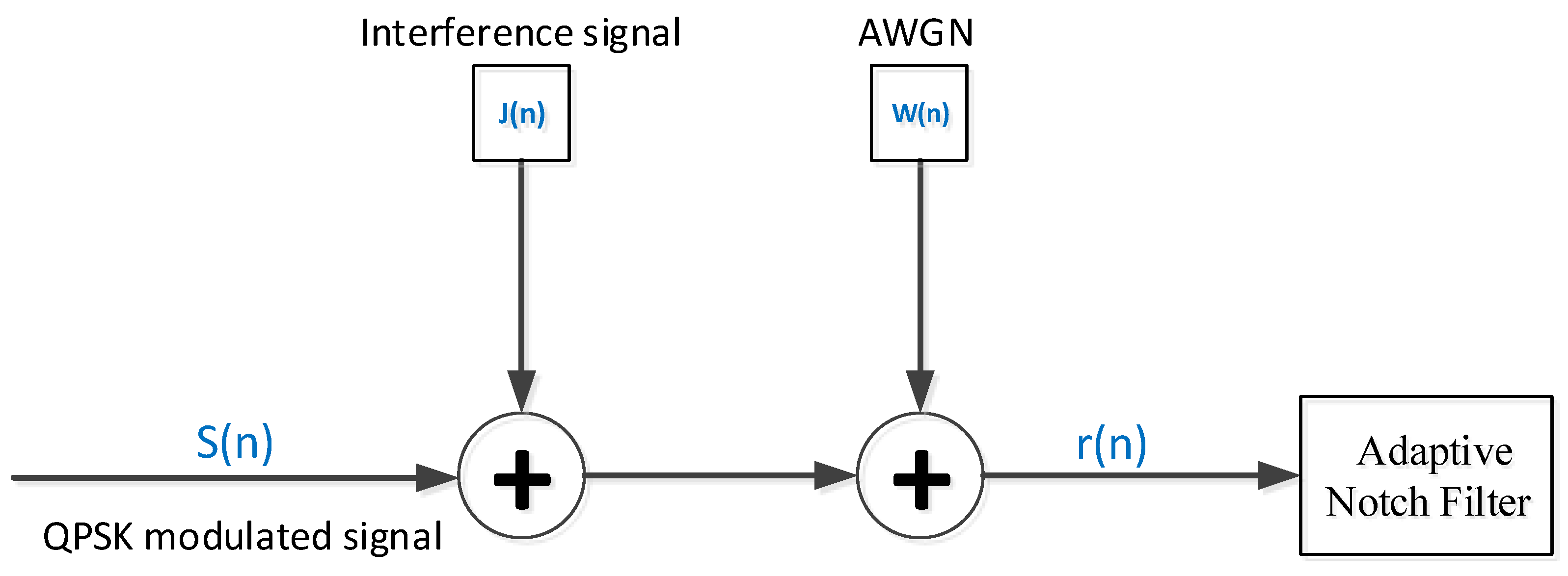
3. Signal Model

A block diagram of the system model for a QPSK-received signal is presented in Figure 3, where a MATLAB simulation model is used to generate a QPSK-modulated signal $S\left(t\right)$ and an interference signal $J_i\left(t\right)$ with the Additive White Gaussian Noise (AWGN) $w\left(t\right)$.

Received Signal Model for The QPSK System

For a QPSK system, the received signal, $r\left(t\right),$ is the input signal to the IIR NF, and it consists of a QPSK-modulated signal $S\left(t\right)$ with the interference signal,$J_i\left(t\right)$, and the AWGN, $w\left(t\right)$, as an illustration of our method, and is expressed as:

$$r\left(t\right)=S\left(t\right)+w\left(t\right)+J_i\left(t\right)$$

(1)

where $S\left(t\right)$ is the transmitted signal (QPSK), and has the following format:

$$S\left(t\right)=S_1\left(t\right)+j{S}_2\left(t\right)$$

and $J_i\left(t\right)$ is the interference signal:

$$J_i\left(t\right)=J_{i1}\left(t\right)+j{J}_{i2}\left(t\right)$$

Equation (1), then sampled at the chip rate to convert it into discrete time n, is $r\left(n\right)$, and is expressed as:

$$r\left(n\right)=S\left(n\right)+w\left(n\right)+J_i\left(n\right)$$

(2)

where $J_i\left(t\right)$ can be modeled as:

$$J_i\left(n\right)={\displaystyle \sum }_{i=1}^m{A}_{i}cos\left({\omega }_{i}n+{\theta }_i\right)$$

(3)

• $A_i$ is the unknown amplitude of the $i\mathrm{th}$ interference signal;
• ${\omega }_i$ is the unknown frequency of the $i\mathrm{th}$ interference signal and ${\omega }_i=2\pi f_{i }$;
• ${\theta }_i$ is the phase delay of the $i\mathrm{th}$ interference signal, which is considered to be a random variable uniformly distributed in the range [$-\pi ,\pi ]$;
• $m$ is the number of CW interferences, and n is the time index.

Substituting interference signal $J_i\left(n\right)$ into Equation (2):

$$r\left(n\right)=S\left(n\right)+w\left(n\right)+{\displaystyle \sum }_{i=1}^m{A}_{i}cos\left(2\pi f_{i}n+{\theta }_i\right)$$

(4)

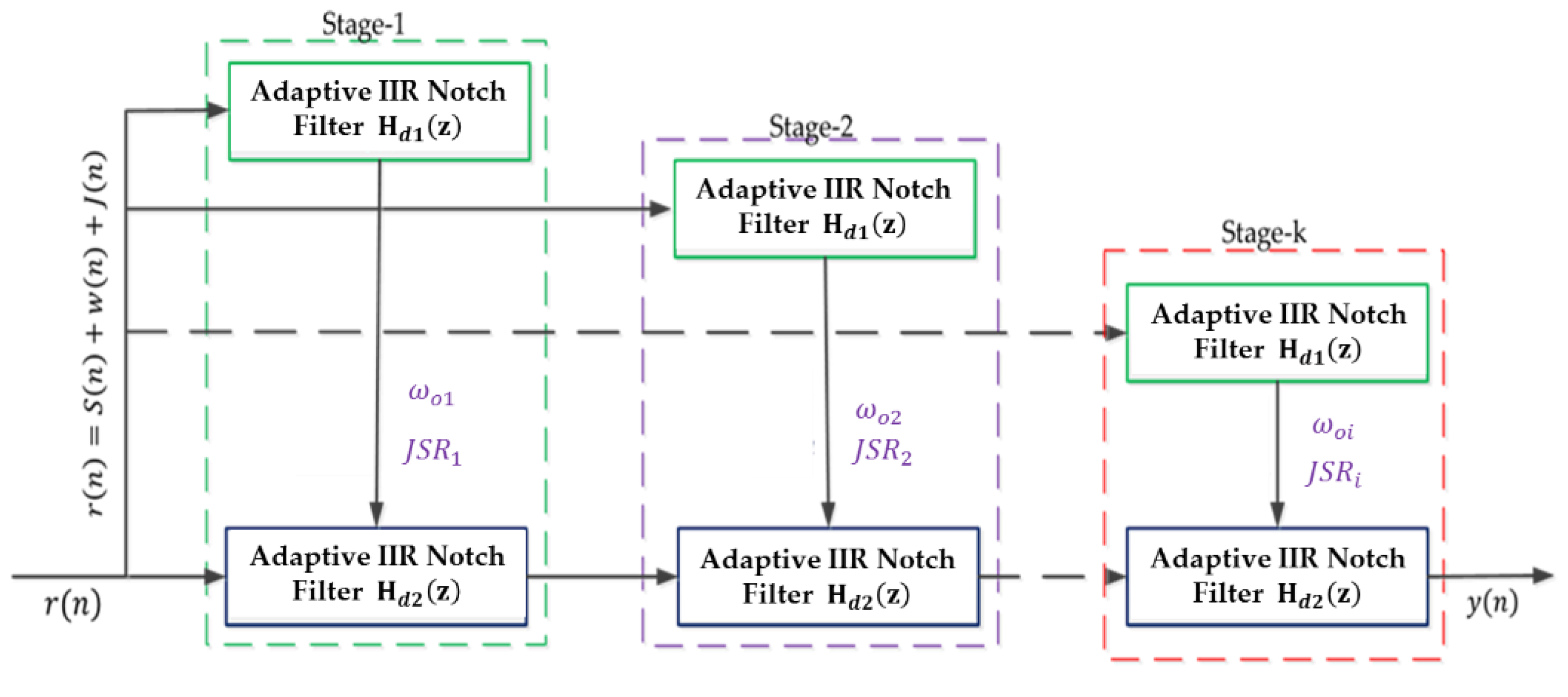
4. Proposed Suppression System Model

This section introduces the structures of the proposed adaptation algorithm for the suppression of CWI and MCWI. The proposed algorithm employs a low-complexity technique for detecting and mitigating CW/MCW interference in the TD. TD is used in order to avoid the drawbacks of the FD approach (i.e., complexity, costs). As previously stated, a deep notch is required for perfect jamming removal in the case of high-power jammers. However, ANFs introduce self-noise, significantly reducing the SNR. Thus, in order to reduce the self-noise, the depth of the notch should be controlled according to the power of the interference. In other words, the depth of the notch should be adjusted with respect to the power of the interference for the trade-off between the information signal distortion and interference reduction. In this paper, a suppression system model is proposed to adjust the depth of the NF based on estimated JSR. The suppression proposed consists of two ANFs based on a second IIR NF direct-form structure—ANF $H_{d1}\left(z\right)$ and ANF $H_{d2}\left(z\right)$—as shown in Figure 4. The ANF $H_{d1}\left(z\right)$ is used in this model to detect and estimate the frequency of the interference (${\omega }_o$) and $JSR$, respectively, through a novel adaptive method as shown in Equation (11) and Equation (13), where the notch’s depth is then adjusted based on the JSR estimation. The ANF $H_{d2}\left(z\right)$ is used to mitigate the CW interference.

To mitigate MCWI, Figure 5 describes the Multiple Adaptive Notch Filter (MANF) model based on the direct-form structure. The MANF model is multistage, with two ANFs in each stage. The structure of each stage can be implemented using the same structure described in Section 4.2.1, modifying the transfer functions $H_{d1}\left(z\right)$ by indicating the adaptive coefficient of the $i\mathrm{th}$ ANF and $H_{d2}\left(z\right).$ The proposed objective is to remove/reduce and maximize the output SNR of the IIR NF, thus improving the system performance.

4.1. Overview of Adaptive Digital Filters Structures

Digital filters are the most widely used technique in the communications, radar, biomedical, and other related fields to solve problems of interference. The adaptive filter can be applied to a variety of structures and realizations. NF passes through all frequencies, except for those in a stop or rejection band centered on a central frequency. NF is defined by two parameters: bandwidth, and central frequency [49]. The bandwidth of an ideal NF should be zero, and the magnitude of the pass band should be one [50]. The Finite Impulse Response (FIR) and the IIR are the two most common types of Adaptive Digital NF (ADNF). FIR filters are also known as Moving Average (MA) filters because they implement a zero-based transfer function. While the Autoregression (AR) and the MA, or ARMA, are frequently used to implement an IIR filter that implements all poles and zero-based transfer functions, the IIR requires fewer filter coefficients to achieve the same notch bandwidth as the FIR. Furthermore, the IIR is more widely used and advantageous than FIR, because it requires less computation. According to [51], an IIR filter can model a pole-zero system more accurately than an FIR filter. In [52], the IIR NF could efficiently remove the CWI or NBI. According to [53], the IIR NF achieves a frequency response that is closer to the ideal NF than an FIR NF of equal length.

4.2. Adaptive IIR NF

The ANF is widely used to estimate and track unknown sinusoid frequencies that have been degraded by noise; it comes in two forms: direct and lattice [54]. This section introduces the structures of the IIR NFs $H_{d1}\left(z\right)$ and $H_{d2}\left(z\right)$ on the direct form. The transfer function $H_{d1}\left(z\right)$ of the second IIR NF with the direct-form structure [15] is defined as in Equation (5), and realized in the direct form shown in Figure 6.

$$H_{d1}\left(z \right)=\frac{N_{d1}(z)}{D_{d1}(Z)}=\frac{1+k_{od}{Z}^{-1}+Z^{-2}}{1+\beta k_{od}{Z}^{-1}+{\beta }^2{Z}^{-2}}$$

(5)

where $\beta$, the pole radius factor, controls the filter’s bandwidth, which is close to but less than 1 in order to ensure the stability of NF, and its value is the interval (0,1). $k_{od}$ is a direct-form IIR NF coefficient parameter that rejects an unknown CWI and is defined as $k_{od}$ = −2 cos(${\omega }_o$). The larger $\beta$, the narrower the NF bandwidth. $H_{d1}\left(z\right)$ is stable if the absolute values of both $\beta$ and $k_{od}$ are less than 1.

4.2.1. Adaptation of Parameter $k_{\mathit{od}}$

In this subsection, the derivation of the new adaptive algorithm for controlling the coefficient of the update filter is utilized using a second IIR NF direct-form structure. Let us assume that the CW interference with the AWGN is added to the QPSK signal as described in Equation (4). $y\left(n\right)$ denotes the output of the $H_{d1}\left(z\right)$, as described in Equation (5), which can be expressed in the TD in terms of the received signal. Thus, the output signal and gradient signal of the second IIR NF are defined as follows:

$$y\left(n\right)=x\left(n\right)+k_{od}x\left(n-1\right)+x\left(n-2\right)-\beta k_{od}\left(n-1\right)-{\beta }^{2}y\left(n-2\right)$$

(6)

The filter’s cost function can be given as in [54]:

$$J\left(k_{od} \right)=E\left\{{\left|y\left(n\right)\right|}^2\right\}$$

(7)

where $E\{\ast \}$ is an expectation operator. Replacing the expectation value in Equation (7) with the ensemble-averaged value as shown in Equation (8), we get:

$$\dot{J}\left(k_{od} \right)=\frac{1}{L}{\displaystyle \sum }_{n=0}^{L-1}{y}^2\left(n\right)$$

(8)

where $L$ is the length of the data. The goal of the filter is to minimize the cost function by adjusting the notch parameter ($k_{od}$) using the gradient-based steepest descent method:

$$k_{od} \left(n+1\right)=k_{od} \left(n\right)-\mu y\left(n\right)\left(g\left(J(k_{od}\right)\right))$$

(9)

where $g\left(J\left(k_{od}\right)\right)$ is the gradient signal of a second ANF based on a direct-form structure for the adaptation of $k_{od},$ and can be expressed as follows:

$$g\left(J\left(k_{od}\right)\right)=\frac{\partial y\left(n\right)}{\partial k_{od}\left(n\right)}=x\left(n-1\right)-\beta y\left(n-1\right)$$

(10)

Substituting Equation (10) into Equation (9):

$$k_{od}\left(n+1\right)=k_{od}\left(n\right)-\mu y\left(n\right)\left(x\left(n-1\right)-\beta y\left(n-1\right)\right)$$

(11)

Equation (11) is the new adaptive algorithm “LMS algorithm” for the proposed ANF that controls the update filter’s coefficient; µ is the step size and the parameter that controls the convergence speed. For stability, k_od ∈ [−2, 2].

Since the normalized notch frequencies, $f_N$ and $k_{od}$, are related by = −2 cos(${\omega }_o$), where ${\omega }_o=2\pi f_N,$ the estimated frequency at sample n can be calculated as follows:

$${\widehat{f}}_N\left(n\right)=\frac{1}{2\pi } Co{s}^{-1}\left(-0.5 k_{od}\left(n\right) \right)$$

(12)

The estimated $JSR$ can be calculated by subtracting the filter’s output $y\left(n\right)$ from the received signal $r\left(n\right),$ and is given as follows:

$$JS{R}_{ dB}=10lo{g}_{10}\left\{{\left|r\left[n\right]-y[n]\right|}^2\right\}$$

(13)

To mitigate the CW interfering signal, a direct-form adaptive IIR NF is used, whose transfer function is given as follows:

$$H_{d2}\left(z\right)=\frac{N_{d2}(z)}{D_{d2}(Z)}=\frac{1+k_{od}\left(k_1\right)Z^{-1}+k_1{Z}^{-2}}{1+k_{od}\left(\beta k_1\right)Z^{-1}+{\beta }^2{k}_1{Z}^{-2}}$$

(14)

where $k_1$ is the notch depth, and is a function of the estimated $JSR$; $\beta$ is the radius of the pole that determines the width of the second IIR NF, as shown in Figure 7 and Figure 8. As stated previously, many implementation schemes can obtain $H_{d2}\left(z\right)$, but in this work, the transfer function $H_{d2}\left(z\right)$ is implemented by cascading all-pole and all-zero direct IIR NF. Note that the setting $k_1=1$ in Equation (14) results in $H_{d2}\left(z\right)\equiv H_{d1}\left(z\right)$, as in Equation (5); hence, the same structure can be used to implement $H_{d2}\left(z\right)$. By copying the $k_{od}$ of $H_{d1}\left(z\right)$, which is tuned to the IF by Equation (11), the notch of Equation (14) can be placed on the IF. As shown in Figure 8, the amount of reduction is a function of the depth of the notch. In the case of $k_1=1$, $H_{d2}\left(z\right)$ is the same as $H_{d1}\left(z\right)$, which has zero on the unit circle and an infinite notch depth, removing all interference caused by excluding some useful signals. Therefore, in order to reduce signal distortion, the depth of the notch $k_1$ should be adjusted with respect to the estimated JSR. To maximize the output SNR, the parameters $\mathrm{JSR}$, $k_{od}$, and $k_1$ are required when designing $H_{d2}\left(z\right)$.

4.2.2. Optimal Notch Depth, Maximizing the Output SNR

In this subsection, the output SNR of the second IIR NF is expressed as a function of its parameters. Moreover, we describe how to obtain the optimal notch depth value $\left(k_1\right)$ that maximizes the $SN{R}_o dB$, as follows:

$$SN{R}_{o}dB=10{\log }_{10}(\frac{E\left[S^2\left(n\right)\right]}{E\left[{\left(y\left(n\right)-S\left(n\right)\right)}^2\right]})$$

(15)

where $y\left(n\right)$ is the output of the second IIR NF $H_{d2}\left(z\right)$, which is expressed as follows:

$$y\left(n\right)=H_{d2}\left(z\right)r\left(n\right)\triangleq S_o\left(n\right)+w_o\left(n\right)+J_o\left(n\right)$$

(16)

where $S_o\left(n\right)$, $w_o\left(n\right)$, and $J_o\left(n\right)$ are the output components of the desired QPSK-modulated signal, the AWGN, and the CWI, respectively. $S_o\left(n\right)$ is a distorted version of the information signal $S\left(n\right)$ caused by information removal at the notch frequency of $H_{d2}\left(z\right)$.

$$E\left[{\left(y\left(n\right)-S\left(n\right)\right)}^2\right]=E\left[y^2\left(n\right)\right]-2E\left[y\left(n\right)S\left(n\right)\right]+E\left[S^2\left(n\right)\right]$$

(17)

Since $E\left[S^2\left(n\right)\right]$= 1 is obtained after normalization, Equation (17) becomes:

$$E\left[{\left(y\left(n\right)-S\left(n\right)\right)}^2\right]=E\left[y^2\left(n\right)\right]-2E\left[y\left(n\right)S\left(n\right)\right]+1$$

(18)

To express $SN{R}_o dB$ as a function of the parameters of the second IIR NF, $E\left[y^2\left(n\right)\right]$ and $E\left[y\left(n\right)S\left(n\right)\right]$ can be expressed with respect to filter parameters by assuming that $S_o\left(n\right),w_o\left(n\right), and J_o\left(n\right)$ are independent and expressing them as a function of the parameters of the second IIR NF:

$$E\left[y^2\left(n\right)\right]=E[{\left(S_o\left(n\right)+w_o\left(n\right)+J_o\left(n\right)\right)}^2]$$

(19)

$$E\left[y^2\left(n\right)\right]=E\left[S_o{}^2\left(n\right)\right]+E\left[w_o{}^2\left(n\right)\right]+E\left[J_o{}^2\left(n\right)\right]$$

(20)

The components ($S_o\left(n\right),w_o\left(n\right), and J_o\left(n\right)$) are independent of one another; thus, other terms will be equal to zero. Equation (20) can therefore be expressed as follows:

$$E\left[y^2\left(n\right)\right]={{\displaystyle \sum }}_{k=0}^{\infty }{h}_k{}^2+{\sigma }_{w_o}{}^2+{\sigma }_{J_o}{}^2$$

(21)

where $h_k$ is the impulse response of the second IIR NF, while ${\sigma }_{w_o}{}^2$ and ${\sigma }_{J_o}{}^2$ are variances of $w_o\left(n\right) and J_o\left(n\right)$, respectively. $E\left[y\left(n\right)S\left(n\right)\right]$ can be expressed as follows:

$$\begin{gathered} E\left[y\left(n\right)S\left(n\right)\right]=E\left[\left(S_o\left(n\right)+w_o\left(n\right)+J_o\left(n\right)\right)S\left(n\right)\right] \\ =E[\left(S_o\left(n\right) S\left(n\right)\right]=h_o \end{gathered}$$

(22)

Substituting Equations (21) and (22) into Equation (18):

$$E\left[{\left(y\left(n\right)-S\left(n\right)\right)}^2\right]={{\displaystyle \sum }}_{k=0}^{\infty }{h}_k{}^2+{\sigma }_{w_o}{}^2+{\sigma }_{J_o}{}^2-2h_o+1$$

(23)

Then, substituting Equation (23) into Equation (15), note that $h_o=1$

$$SN{R}_{o}dB=10{\log }_{10}(\frac{1}{{{\displaystyle \sum }}_{k=0}^{\infty }{h}_k{}^2+{\sigma }_{w_o}{}^2+{\sigma }_{J_o}{}^2-1})$$

(24)

As stated previously, in order to express $SN{R}_o$ as a function of the parameters of the second IIR NF in Equation (24), we first define $u\left(n\right)$ as the output of $\frac{1}{D_{d2}(Z)}$ with input signal $w\left(n\right):$

$$u\left(n\right)=\frac{1}{D_{d2}(Z)}w\left(n\right)$$

(25)

where $D_{d2}(Z)$ is the all-pole of the second IIR NF, as in Equation (14).

Let $R_{uu}\left(m\right)$ be the autocorrelation of $u\left(n\right),$ i.e., $E\left[u\left(n\right)u\left(n-m\right)\right]$; $R_{uu}\left(0\right)$, $R_{uu}\left(1\right)$, and $R_{uu}\left(2\right)$ can then be expressed as follows [54]:

$$R_{uu}\left(0\right)=E\left[u\left(n\right)u\left(n\right)\right]= \frac{1}{\left(1-{\beta }^2{k}_1^2\right)\left(1-k_{od}^2\right)} {\sigma }^2$$

(26)

$$R_{uu}\left(1\right)=E\left[u\left(n\right)u\left(n-1\right)\right]= \frac{-k_{od}}{\left(1-{\beta }^2{k}_1^2\right) \left(1-k_{od}^2\right)} {\sigma }^2$$

(27)

$$R_{uu}\left(2\right)=E\left[u\left(n\right)u\left(n-2\right)\right]== \frac{k_{\mathit{od}}^2\beta k_1-{\beta }^2{k}_1}{\left(1-{\beta }^2{k}_1^2\right) \left(1-k_{od}^2\right)} {\sigma }^2$$

(28)

where ${\sigma }_{w_o}^2=E\left[w_o^2\left(n\right)\right]$. Since $w_o\left(n\right)=N_{d2}(z)u\left(n\right)$, $w_o\left(n\right)$ can then be expressed as follows:

$$w_o\left(n\right)=\left(1+k_{od}{k}_1{Z}^{-1}+k_1{Z}^{-2}\right)u\left(n\right)$$

(29)

$$w_o\left(n\right)=u\left(n\right)+k_{od}{k}_{1}u\left(n-1\right)+k_{1}u\left(n-2\right)$$

(30)

The variance of $w_o\left(n\right)$ is given by ${\sigma }_{w_o}^2=E\left[w_o^2\left(n\right)\right]$; thus:

$$\begin{gathered} {\sigma }_{w_o}^2=E[{\left(u\left(n\right)+k_{od}{k}_{1}u\left(n-1\right)+k_{1}u\left(n-2\right)\right)}^2] \\ {\sigma }_{w_o}^2=\left\{1+k_{od}^2{k}_1{}^2+k_1{}^2\right\}{R}_{uu}\left(0\right)+\left\{2k_{od}{k}_1\right(1+k_1\left)\right\}{R}_{uu}\left(1\right)+2k_1{R}_{uu}\left(2\right) \end{gathered}$$

(31)

Substituting Equations (26)–(28) into Equation (31), the ${\sigma }_{w_o}^2$ becomes:

$${\sigma }_{w_o}^2=\frac{1+k_1^2-2{\beta }^2{k}_1^2}{\left(1-{\beta }^2{k}_1^2\right)}{\sigma }^2$$

(32)

Moreover, since ${\sigma }_{w_o}^2=E\left[w_o^2\left(n\right)\right]={\sigma }^2{{\displaystyle \sum }}_{k=0}^{\infty }{h}_k^2$, we have:

$${{\displaystyle \sum }}_{k=0}^{\infty }{h}_k^2=\frac{1+k_1^2-2{\beta }^2{k}_1^2}{\left(1-{\beta }^2{k}_1^2\right)}$$

(33)

${\sigma }_{J_o}{}^2$ in Equation (24) is the interference power after the second IIR NF, since $J_o\left(n\right)$ CWI with center frequency ${\omega }_o$, the variance of $J_o\left(n\right)$ is given as follows:

$${\sigma }_{J_o}{}^2=\frac{A^2}{2}{\left|H\left(e^{j{\omega }_o}\right)\right|}^2$$

(34)

When the adaptive algorithms in Equation (6) and Equation (11) are successfully converged, $k_{od}$ = −2 cos(${\omega }_o$), and Equation (34) becomes:

$${\sigma }_{J_o}{}^2=\frac{A^2}{2}\frac{{\left(1-k_1\right)}^2}{{\left(1-\beta k_1\right)}^2}$$

(35)

Hence, substituting Equations (32), (33), and (35) into Equation (24) yields the described $SN{R}_{o }dB$ in terms of filter parameters, as follows:

$$SN{R}_{o}dB=10{\log }_{10}(\frac{1}{\left(1+{\sigma }^2\right)\left(\frac{1+k_1^2-2{\beta }^2{k}_1^2}{\left(1-{\beta }^2{k}_1^2\right)}\right)+JS{R}_i\left(\frac{{\left(1-k_1\right)}^2}{{\left(1-\beta k_1\right)}^2}\right)-1})$$

(36)

where ${\sigma }^2$ is the variance of AWGN, and $JS{R}_i=\frac{A_i^2}{2}$.

To maximize $SN{R}_o dB$ in Equation (36), the optimal value $k_1$ needs to be found. After some modifications, the denominator in Equation (36) can be rewritten as a function of $k_1$:

$$f{(k}_1)=\left(\frac{1+k_1^2-2{\beta }^2{k}_1^2}{\left(1-{\beta }^2{k}_1^2\right)}\right)+G_i\left(\frac{{\left(1-k_1\right)}^2}{{\left(1-\beta k_1\right)}^2}\right)-\frac{1}{\left(1+{\sigma }^2\right)}$$

(37)

where $G_i=\frac{JS{R}_i}{\left(1+{\sigma }^2\right)}$. To find the optimal $k_1$, we differentiate $f{(k}_1)$ and solve $f^{\prime }\left(k_1\right)=0$ for all possible roots of $k_1,$ as shown in Equation (37):

$$f^{\prime }\left(k_i\right)={\beta }^2{G}_i{k}_1^3+\left[2\beta G_i-{\beta }^2{G}_i-{\beta }^2-\beta \right]k_1^2+\left[1+\beta +G_i-2\beta G\right]k_1-G_i=0$$

(38)

Equation (38) has at least one real root in the [0 1] range that gives the optimal $k_1$ as a function of $JS{R}_i$.

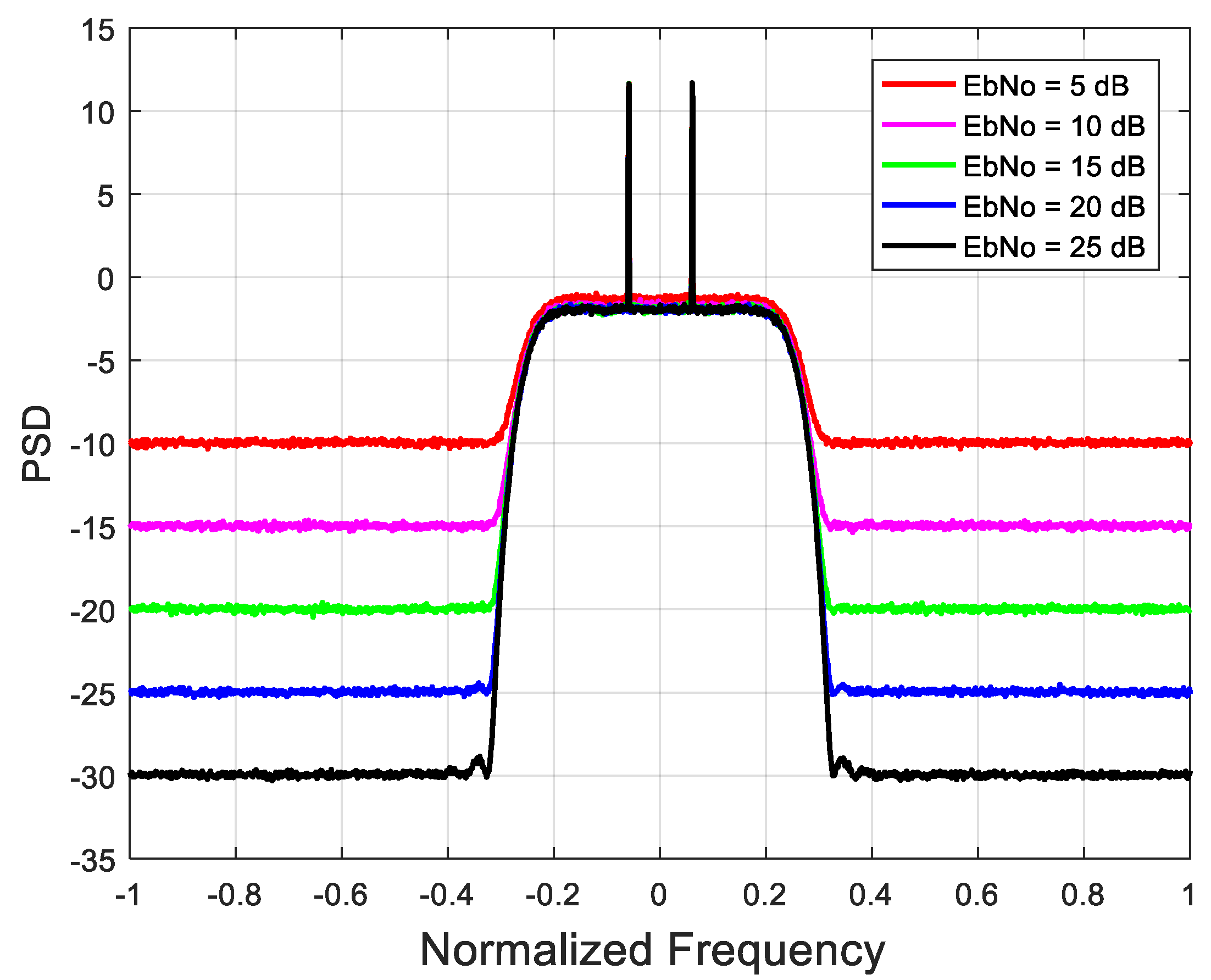
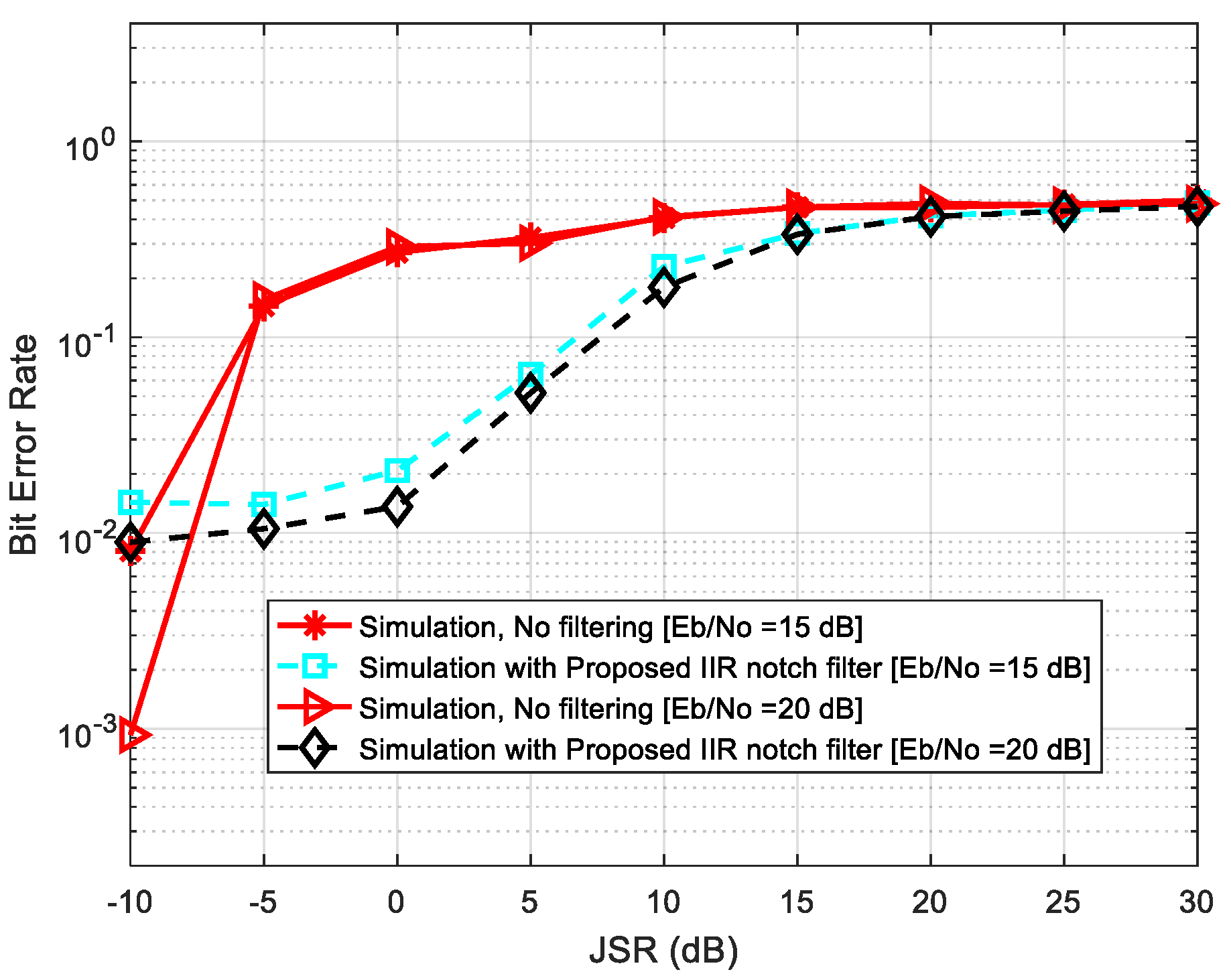
5. Simulation Results and Discussion

This section discusses the performance of the proposed adaptation algorithm for CWI and MCWI suppression scenarios. The proposed algorithm uses a second IIR NF based on a direct-form structure to control the update filter coefficient and notch depth in the TD. The ${\mathit{SNR}}_o\mathit{dB}$ and the BER are used to evaluate the system performance for the proposed algorithm in terms of varying the SOI power ($E_b/N_o$) and JSR. In this work, the number of CWIs is considered to be 2 for the $i\mathrm{th}$ jamming signal, with center frequencies ($f_1=0.03$ and $f_2=0.08$) and with an unknown amplitude ($A_i$). The simulation was run for 1e7 data bits to mitigate CWI and MCWI. β was set to 0.98 in order to provide more acceptable outcomes in various scenarios. There was a trade-off between some properties of ANF $H_{d1}\left(z\right)$ and ANF $H_{d2}\left(z\right)$, and β was chosen. A large β value gave more accurate frequency estimates and JSR, but slower convergence and tracking [54] in $H_{d1}\left(z\right)$. However, for $H_{d2}\left(z\right)$, a large β gave a larger NB noise at the output but a smaller broadband noise [40]. The BER was quantified in terms of JSR changes. All simulation results were obtained using ${\mathrm{MATLAB}}^{\circledR }$ software.

In Figure 9, the notch depth is a function of the estimated JSR. As the JSR increases, the magnitude of the notch depth and bandwidth decreases. The CWI’s power determines the depth of the notch magnitude response—the higher the CWI’s power, the deeper the notch magnitude response.

The BER performance as E_b/N_o changes is depicted in the figures below. In the simulations, various values of $E_b/N_o$ and a constant value of JSR were used. Figure 10 and Figure 11 illustrate the performance in the presence of CW and MCW interference, with a constant JSR, and controlling the depth of the NF with respect to estimating the power of interference. The results demonstrate that the proposed IIR NF achieves a better BER with CWI—especially when the JSR is small or large, as shown in Figure 12 and Figure 13, respectively. Thus, the ANF can reduce interference and obtain a better BER.

Figure 14 and Figure 15 show the BER performance with variations of the JSR. Simulations were carried out with various JSR values and a constant value of E_b/N_o, while adjusting the depth of the NF. The simulation results were compared between the proposed IIR NF (filtering) and no filtering cases; they show that the proposed algorithm outperforms the no filtering in the case of filtering. Figure 16 and Figure 17 illustrate the proposed ANF algorithm in comparison with full suppression ($k_1=1$) while using a Single Adaptive IIR NF (S-ANF) and Multiple Adaptive NFs (MANF). The notch depth was efficiently controlled by the proposed algorithm, and achieved better results than full suppression for both low and high JSR.

Figure 18 and Figure 19 show the performance of the SNR vs. the JSR. The proposed IIR NF algorithm efficiently adjusts the notch depth in each step, making it deeper for a high JSR. In the latter case, the results show that full suppression outperforms the case without an NF (no filtering), indicating that full suppression is better for a high JSR, while no filtering is better for a low JSR. This further illustrates that the proposed IIR NF approaches full suppression when the JSR increases (irrespective of the stage), because the notch depth deepens in this case; thus, the notch depth becomes smaller for a lower JSR value and deeper for a higher JSR value.

Figure 20 depicts the Power Spectrum (PS)-received signal before and after IIR NF processing. The results indicate that the proposed method is capable of detecting and mitigating CWI; they also show that by adjusting the depth of the NF, the CWI is removed according to the estimated JSR, which prevents the Signal of Interest (SoI) from being reduced.

Most of the previous studies introduced in this paper emphasize the suppression of CWI and MCWI without focusing on adjusting the depth of the NF. These methods completely remove the interference, but they generate a significant amount of self-noise, which causes the distortion of some useful signals. In order to reduce the loss of some useful signals while removing interference, we proposed a low-complexity algorithm that uses a second-order IIR NF based on a direct-form structure to estimate the JSR by adjusting and controlling the depth of the NF, which has not been considered in previous studies—particularly [11]. Moreover, according to the comparison of the IIR NF with a lattice-form structure, as shown in Figure 21, we observed that the IIR notch filter with a direct-form structure outperforms the IIR notch filter with a lattice-form structure for detection and removal in the case of high-power jamming. Furthermore, by comparing the direct form with a lattice form, as shown in Figure 22, we can see that $k_1$ approaches 1 for both the direct and lattice notch filters as the JSR increases. However, for the lattice-form filter, $k_1$ approaches 1 faster than in the case of the direct-form filter at the same $E_b/N_o$ parameters. In other words, for the lattice-form filter, $k_1$ jumps to 1 even at small values of CWI in comparison to the direct-form filter, affecting the quality of the useful signal.

6. Conclusions

This paper proposes a new adaptive algorithm that controls the update filter coefficient and adjusts the notch depth with respect to JSR. Moreover, the proposed method detects and cancels single and multiple interferences using an ANF based on a second IIR direct NF. The proposed algorithms operate in TD, which eliminates the need for transferred domain information and, thus, lowers hardware costs. Furthermore, by cascading MANF modules, the proposed ANF module can notch out multiple CWIs. Simulation results show that as JSR increases, the notch bandwidth decreases, as does the depth of the notch magnitude responses. Therefore, the proposed approach can detect and mitigate interference while adjusting the notch depth for any given JSR values, effectively controlling the notch depth; it also achieves better performance than full suppression for both low and high JSR values. The results indicate that the IIR NF can adapt, track any frequency change, and reduce CWI power at the output of the NF, with less distortion of the useful signal; they also clearly show improvements over ANF in terms of overall BER, as well as a robust performance of the ANF over a range of JSR values—especially in terms of CWI. This method is able to detect and mitigate weak and the strong jamming (−30 to 40 dB); therefore, it can be used in a DVB-S2 receiver, or in other types of wireless communication receivers.

References

- Wyatt, K.; Gruber, M. Radio Frequency Interference (RFI) Pocket Guide; Scitech Publishing: Raleigh, NC, USA, 2015. [Google Scholar] [CrossRef]
- Elbert, B. Radio Frequency Interference in Communications Systems; Artech House: London, UK, 2016. [Google Scholar]
- Mpitziopoulos, A.; Gavalas, D.; Konstantopoulos, C.; Pantziou, G. A survey on jamming attacks and countermeasures in WSNs. IEEE Commun. Surv. Tutor. 2009, 11, 42–56. [Google Scholar] [CrossRef]
- Grover, K.; Lim, A.; Yang, Q. Jamming and anti-jamming techniques in wireless networks: A survey. Int. J. Ad Hoc Ubiquitous Comput. 2014, 17, 197–215. [Google Scholar] [CrossRef] [Green Version]
- Shahriar, C.; La Pan, M.; Lichtman, M.; Clancy, T.C.; McGwier, R.; Tandon, R.; Sodagari, S.; Reed, J.H. PHY-layer resiliency in OFDM communications: A tutorial. IEEE Commun. Surv. Tutor. 2014, 17, 292–314. [Google Scholar] [CrossRef]
- Wei, X.; Wang, Q.; Wang, T.; Fan, J. Jammer localization in multi-hop wireless network: A comprehensive survey. IEEE Commun. Surv. Tutor. 2016, 19, 765–799. [Google Scholar] [CrossRef]
- Lichtman, M.; Jover, R.P.; Labib, M.; Rao, R.; Marojevic, V.; Reed, J.H. LTE/LTE-A jamming, spoofing, and sniffing: Threat assessment and mitigation. IEEE Commun. Mag. 2016, 54, 54–61. [Google Scholar] [CrossRef]
- Borio, D.; Dovis, F.; Kuusniemi, H.; Presti, L.L. Impact and detection of GNSS jammers on consumer grade satellite navigation receivers. Proc. IEEE 2016, 104, 1233–1245. [Google Scholar] [CrossRef]
- Qin, W.; Gamba, M.T.; Falletti, E.; Dovis, F. An assessment of impact of adaptive notch filters for interference removal on the signal processing stages of a GNSS receiver. IEEE Trans. Aerosp. Electron. Syst. 2020, 56, 4067–4082. [Google Scholar] [CrossRef]
- Getu, T.M.; Ajib, W.; Landry, R. INR walls: Performance limits in RFI detection. In Proceedings of the 2019 IEEE 30th Annual International Symposium on Personal, Indoor and Mobile Radio Communications (PIMRC), Istanbul, Turkey, 8–11 September 2019; pp. 1–6. [Google Scholar]
- Same, M.; Gleeton, G.; Gandubert, G.; Ivanov, P.; Landry, R. Multiple narrowband interferences characterization, detection and mitigation using simplified welch algorithm and notch filtering. Appl. Sci. 2021, 11, 1331. [Google Scholar] [CrossRef]
- ETSI EN 302 307-1 V1. 4.1; Second Generation Framing Structure, Channel Coding and Modulation Systems for Broadcasting, Interactive Services, News Gathering and Other Broadband Satellite Applications. Digital Video Broadcasting: Geneva, Switzerland, 2014.
- Cho, N.I.; Choi, C.H.; Lee, S.U. Adaptive line enhancement by using an IIR lattice notch filter. IEEE Trans. Acoust. Speech Signal Process. 1989, 37, 585–589. [Google Scholar]
- Borio, D.; Camoriano, L.; Savasta, S.; Presti, L.L. Time-frequency excision for GNSS applications. IEEE Syst. J. 2008, 2, 27–37. [Google Scholar] [CrossRef]
- Choi, J.W.; Cho, N.I. Narrow-band interference suppression in direct sequence spread spectrum systems using a lattice IIR notch filter. In Proceedings of the 2001 IEEE International Conference on Acoustics, Speech and Signal Processing, Salt Lake City, UT, USA, 7–11 May 2001; Volume 4, pp. 2237–2240. [Google Scholar] [CrossRef]
- Stearns, S.D. Fundamentals of Adaptive Signal Processing. Available online: https://course.ece.cmu.edu/~ece792/handouts/LO_Chap_AdaptiveFilters.pdf (accessed on 18 January 2022).
- Ferdjallah, M.; Barr, R. Adaptive digital notch filter design on the unit circle for the removal of powerline noise from biomedical signals. IEEE Trans. Biomed. Eng. 1994, 41, 529–536. [Google Scholar] [CrossRef]
- Borio, D.; Camoriano, L.; Presti, L.L. Two-pole and multi-pole notch filters: A computationally effective solution for GNSS interference detection and mitigation. IEEE Syst. J. 2008, 2, 38–47. [Google Scholar] [CrossRef]
- Kuo, S.; Chen, J. New adaptive IIR notch filter and its application to howling control in speakerphone system. Electron. Lett. 1992, 28, 764–766. [Google Scholar] [CrossRef]
- Lu, D.; Wu, R.; Liu, H. Global positioning system anti-jamming algorithm based on period repetitive CLEAN. IET Radar Sonar Navig. 2013, 7, 164–169. [Google Scholar] [CrossRef]
- Lin, T.; Abdizadeh, M.; Broumandan, A.; Wang, D.; O’Keefe, K.; Lachapelle, G. Interference suppression for high precision navigation using vector-based GNSS software receivers. In Proceedings of the 24th International Technical Meeting of The Satellite Division of the Institute of Navigation (ION GNSS 2011), Portland, OR, USA, 20–23 September 2011; pp. 372–383. [Google Scholar]
- Glennon, E.P.; Dempster, A.G. Delayed PIC for postcorrelation mitigation of continuous wave and multiple access interference in GPS receivers. IEEE Trans. Aerosp. Electron. Syst. 2011, 47, 2544–2557. [Google Scholar] [CrossRef]
- Barbarossa, S.; Scaglione, A. Adaptive time-varying cancellation of wideband interferences in spread-spectrum communications based on time-frequency distributions. IEEE Trans. Signal Process. 1999, 47, 957–965. [Google Scholar] [CrossRef] [Green Version]
- Ma, W.-J.; Mao, W.-L.; Chang, F.-R. Design of adaptive all-pass based notch filter for narrowband anti-jamming GPS system. In Proceedings of the 2005 IEEE International Symposium on Intelligent Signal Processing and Communication Systems, Hong Kong, China, 13–16 December 2005; pp. 305–308. [Google Scholar]
- Zhang, Y.D.; Amin, M.G. Anti-jamming GPS receiver with reduced phase distortions. IEEE Signal Process. Lett. 2012, 19, 635–638. [Google Scholar] [CrossRef]
- Higgins, T.S.; Webster, T.; Shackelford, A.K. Mitigating interference via spatial and spectral nulls. In Proceedings of the IET International Conference on Radar Systems, Glasgow, UK, 22–25 October 2012. [Google Scholar] [CrossRef]
- Azarbad, M.R.; Mosavi, M.R. A new method to mitigate multipath error in single-frequency GPS receiver with wavelet transform. GPS Solut. 2014, 18, 189–198. [Google Scholar] [CrossRef]
- Zhang, Y.; Amin, M.G.; Lindsey, A.R. Anti-jamming GPS receivers based on bilinear signal distributions. In 2001 MILCOM Communications for Network-Centric Operations: Creating the Information Force (Cat. No. 01CH37277), Proceedings of the MILCOM, Military Communications Conference, McLean, VA, USA, 28–31 October 2001; IEEE: New York, NY, USA, 2001; Volume 2, pp. 1070–1074. [Google Scholar]
- Jiang, F.-W.; Xiao, Z.; Yi, K.-C.; Sun, Y.-J. Adaptive two-stage filter bank based narrowband interference suppression in DSSS systems. In Proceedings of the 9th IEEE International Conference on Signal Processing, Beijing, China, 26–29 October 2008; pp. 88–91. [Google Scholar] [CrossRef]
- Ouyang, X.; Amin, M. Short-time Fourier transform receiver for nonstationary interference excision in direct sequence spread spectrum communications. IEEE Trans. Signal Process. 2001, 49, 851–863. [Google Scholar] [CrossRef]
- Landry, R.J.R.; Mouyon, P.; Lekaïm, D. Interference mitigation in spread spectrum systems by wavelet coefficients thresholding. Eur. Trans. Telecommun. 1998, 9, 191–202. [Google Scholar] [CrossRef]
- Dovis, F.; Musumeci, L. Use of wavelet transforms for interference mitigation. In Proceedings of the 2011 International Conference on Localization and GNSS (ICL-GNSS), Tampere, Finland, 29–30 June 2011; pp. 116–121. [Google Scholar]
- Solano, J.J.P.; Felici-Castell, S.; Rodriguez-Hernandez, M.A. Narrowband interference suppression in frequency-hopping spread spectrum using undecimated wavelet packet transform. IEEE Trans. Veh. Technol. 2008, 57, 1620–1629. [Google Scholar] [CrossRef]
- Mosavi, M.R.; Pashaian, M.; Rezaei, M.J.; Mohammadi, K. Jamming mitigation in global positioning system receivers using wavelet packet coefficients thresholding. IET Signal Process. 2015, 9, 457–464. [Google Scholar] [CrossRef]
- Lotz, T. Adaptive Analog-to-Digital Conversion and Pre-Correlation Interference Mitigation Techniques in a GNSS Receiver. Master’s Thesis, Technical University of Kaiserslautern, Kaiserslanutern, Germany, 2008. [Google Scholar]
- Balaei, A.T.; Dempster, A. A statistical inference technique for GPS interference detection. IEEE Trans. Aerosp. Electron. Syst. 2009, 45, 1499–1511. [Google Scholar] [CrossRef]
- Chien, Y.-R. Design of GPS anti-jamming systems using adaptive notch filters. IEEE Syst. J. 2013, 9, 451–460. [Google Scholar] [CrossRef]
- Wang, H.; Chang, Q.; Xu, Y.; Li, X. Adaptive narrow-band interference suppression and performance evaluation based on code-aided in GNSS inter-satellite links. IEEE Syst. J. 2019, 14, 538–547. [Google Scholar] [CrossRef]
- Choi, J.W.; Cho, N.I. Suppression of narrow-band interference in DS-spread spectrum systems using adaptive IIR notch filter. Signal Process. 2002, 82, 2003–2013. [Google Scholar] [CrossRef]
- Lv, Q.; Qin, H. General method to mitigate the continuous wave interference and narrowband interference for GNSS receivers. IET Radar Sonar Navig. 2020, 14, 1430–1435. [Google Scholar] [CrossRef]
- El Gebali, A.; Landry, R., Jr. Mitigation of continuous wave narrow-band interference in QPSK demodulation using adaptive IIR notch filter. Am. J. Signal Process. 2020, 10, 10–18. [Google Scholar]
- Mosavi, M.R.; Moghaddasi, M.S.; Rezaei, M.J. A new method for continuous wave interference mitigation in single-frequency GPS receivers. Wirel. Pers. Commun. 2016, 90, 1563–1578. [Google Scholar] [CrossRef]
- El Gebali, A.; Landry, R.J. Multi-frequency interference detection and mitigation using multiple adaptive IIR notch filter with lattice structure. J. Comput. Commun. 2021, 9, 58–77. [Google Scholar] [CrossRef]
- Mao, W.-L. Novel SREKF-based recurrent neural predictor for narrowband/FM interference rejection in GPS. AEU-Int. J. Electron. Commun. 2008, 62, 216–222. [Google Scholar] [CrossRef]
- Mao, W.-L.; Ma, W.-J.; Chien, Y.-R.; Ku, C.-H. New adaptive all-pass based notch filter for narrowband/FM anti-jamming GPS receivers. Circuits Syst. Signal Process. 2011, 30, 527–542. [Google Scholar] [CrossRef]
- Vijayan, R.; Poor, H. Nonlinear techniques for interference suppression in spread-spectrum systems. IEEE Trans. Commun. 1990, 38, 1060–1065. [Google Scholar] [CrossRef]
- Mosavi, M.R.; Shafiee, F. Narrowband interference suppression for GPS navigation using neural networks. GPS Solut. 2016, 20, 341–351. [Google Scholar] [CrossRef]
- Rao, K.D.; Swamy, M.; Plotkin, E. A nonlinear adaptive filter for narrowband interference mitigation in spread spectrum systems. Signal Process. 2005, 85, 625–635. [Google Scholar] [CrossRef]
- Landry, R.; Calmettes, V.; Bousquet, M. Impact of interference on a generic GPS receiver and assessment of mitigation techniques. In Proceedings of the IEEE 5th International Symposium on Spread Spectrum Techniques and Applications, Sun City, South Africa, 4 September 1998; Volume 1, pp. 87–91. [Google Scholar] [CrossRef]
- Wang, X.L.; Ge, Y.J.; Zhang, J.J.; Song, Q.J. Discussion on the -3dB rejection bandwidth of IIR notch filters. In Proceedings of the IEEE 6th International Conference on Signal Processing for Wireless Communications, Beijing, China, 26–30 August 2002. [Google Scholar]
- Shynk, J.J. Adaptive IIR filtering. IEEE ASSP Mag. 1989, 6, 4–21. [Google Scholar] [CrossRef]
- Regalia, P.A. Adaptive IIR Filtering in Signal Processing and Control; Routledge: Boca Raton, FL, USA, 2018. [Google Scholar] [CrossRef]
- Punchalard, R. On adaptive IIR lattice notch filter using a robust variable step-size for the detection of sinusoid. In Proceedings of the 8th IEEE International Conference on Communication Systems (ICCS), Singapore, 28 November 2002; pp. 800–804. [Google Scholar] [CrossRef]
- Cho, N.I.; Lee, S.U. On the adaptive lattice notch filter for the detection of sinusoids. IEEE Trans. Circuits and Syst II Analog Digital Signal Process. 1993, 40, 405–416. [Google Scholar] [CrossRef]
Publisher’s Note: MDPI stays neutral with regard to jurisdictional claims in published maps and institutional affiliations. |
© 2022 by the authors. Licensee MDPI, Basel, Switzerland. This article is an open access article distributed under the terms and conditions of the Creative Commons Attribution (CC BY) license (https://creativecommons.org/licenses/by/4.0/).
Share and Cite
El Gebali, A.; Landry, R.J. Single and Multiple Continuous-Wave Interference Suppression Using Adaptive IIR Notch Filters Based on Direct-Form Structure in a QPSK Communication System. Appl. Sci. 2022, 12, 2186. https://doi.org/10.3390/app12042186
El Gebali A, Landry RJ. Single and Multiple Continuous-Wave Interference Suppression Using Adaptive IIR Notch Filters Based on Direct-Form Structure in a QPSK Communication System. Applied Sciences. 2022; 12(4):2186. https://doi.org/10.3390/app12042186
Chicago/Turabian StyleEl Gebali, Abdelrahman, and René Jr Landry. 2022. "Single and Multiple Continuous-Wave Interference Suppression Using Adaptive IIR Notch Filters Based on Direct-Form Structure in a QPSK Communication System" Applied Sciences 12, no. 4: 2186. https://doi.org/10.3390/app12042186
APA StyleEl Gebali, A., & Landry, R. J. (2022). Single and Multiple Continuous-Wave Interference Suppression Using Adaptive IIR Notch Filters Based on Direct-Form Structure in a QPSK Communication System. Applied Sciences, 12(4), 2186. https://doi.org/10.3390/app12042186