Article

Percussion-Based Pipeline Ponding Detection Using a Convolutional Neural Network

1
Key Laboratory for Metallurgical Equipment and Control of Ministry of Education, Wuhan University of Science and Technology, Wuhan 430081, China
2
Hubei Key Laboratory of Mechanical Transmission and Manufacturing Engineering, Wuhan University of Science and Technology, Wuhan 430081, China
3
Precision Manufacturing Institute, Wuhan University of Science and Technology, Wuhan 430081, China
*
Author to whom correspondence should be addressed.
Appl. Sci. 2022, 12(4), 2127; https://doi.org/10.3390/app12042127
Submission received: 20 January 2022 / Revised: 8 February 2022 / Accepted: 16 February 2022 / Published: 18 February 2022

Abstract

:
Pipeline transportation is the main method for long-distance gas transportation; however, ponding in the pipeline can affect transportation efficiency and even cause corrosion to the pipeline in some cases. A non-destructive method to detect pipeline ponding using percussion acoustic signals and a convolution neural network (CNN) is proposed in this paper. During the process of detection, a constant energy spring impact hammer is used to apply an impact on the pipeline, and the percussive acoustic signals are collected. A Mel spectrogram is used to extract the acoustic feature of the percussive acoustic signal with different ponding volumes in the pipeline. The Mel spectrogram is transferred to the input layer of the CNN and the convolutional kernel matrix of the CNN realizes the recognition of pipeline ponding volume. The recognition results show that the CNN can identify the amount of pipeline ponding with the percussive acoustic signals, which use the Mel spectrogram as the acoustic feature. Compared with the support vector machine (SVM) model and the decision tree model, the CNN model has better recognition performance. Therefore, the percussion-based pipeline ponding detection using the convolutional neural network method proposed in this paper has high application potential.

1. Introduction

As a main method of oil and gas transportation, pipelines play an important role in transporting supplies [1,2]. During their long-term service life, various types of pipeline damages are related to pipeline ponding; corrosion, perforation, and leakage are not uncommon, and they usually bring about serious safety hazards to pipeline transportation [3]. Therefore, to ensure the safe and stable operation of pipelines, pipeline ponding detection has become more important and urgent.
In pipeline ponding detection, changes in the ponding volume will cause changes in the structural characteristics of the pipeline system composed of pipeline and ponding. Therefore, some developed methods for the monitoring of structural characteristics may provide an approach as the reference for pipeline ponding detection. In recent decades, several common methods for pipeline structure characteristic detection have been introduced, including the CCTV (closed-circuit television) inspection method [4], the ultrasonic testing method [5] and the radiography method [6]. The CCTV inspection method presents very rich internal information of the pipeline in the form of photos or videos [7] by a robotic system with a camera [8]. However, the CCTV method is greatly affected by environmental factors, and its detection accuracy of the pipeline evaluation depends largely on the quality of the hardware system and the experience of the inspectors [9]. The ultrasonic testing method can estimate the health state by analyzing reflection waves [10,11] in the pipelines. It is sensitive to changes in structural state and can be related to several structural characteristics [12]. However, the signals collected by the ultrasonic method are usually accompanied with noise, and effective noise reduction methods are required to obtain useful information [13,14]. The radiography method detects the pipeline by evaluating the attenuation of the rays [15] which pass through the pipeline. This method can be used for pipelines with complex geometric shapes [16]. However, its detection accuracy decreases when it is employed for vertical angle defect detection [17], and the rays are harmful to human health [18]. Therefore this method’s practical application is very limited.
Compared with the aforementioned detection approaches, the percussive detection method [19,20,21] has the characteristics of deep detection and fast transmission speeds, and is user-friendly [22]. It is used to determine the pipeline structure characteristic by the sounds generated through impact on the pipeline under test [23]. Traditional percussive detection method still requires engineering experience, which can be subjective and inefficient [24]. This is solved by using the powerful computing power of computers or the automatic prediction and classification properties of machine learning. Furui Wang et al. proposed a new percussion-based method using analytical modeling and numerical simulation, whereby a percussion-induced sound pressure level (SPL) could be obtained via the acoustic radiation mode approach. The corresponding numerical simulation was developed with a focus on the acoustic–structure coupling, and the acoustic boundary conditions were satisfied through a perfectly matched layer (PML) [25]. Liqiong Zheng et al. used Mel-frequency cepstral coefficients (MFCCs) as the features of percussion-induced acoustics, and support vector machine (SVM)-based machine learning was utilized to classify results [26]. Dongdong Chen et al. used power spectrum density (PSD) to process percussive sound, and a decision tree machine (DTM) learning approach was used to classify results [27].
CNN, one of the representative algorithms of deep learning, which automatically predicts and classifies the data [28], can overcome the drawbacks of percussive detection methods that requires engineering experience, and can therefore obtain superior results in visual classification tasks [29]. In the classification of audio data, as CNN cannot process sound directly [30], the sound of digital signals is often converted into spectrogram images [31] by a Short-time Fourier transform (STFT) or a wavelet transform. In particular, the STFT is a low-complexity time–frequency method capable of analyzing non-stationary signals which has a low computational burden [32]. However, the dimension of the spectrogram after STFT is relatively high, resulting in a large amount of subsequent CNN calculation, which increases the complexity of CNN learning. Furthermore, a nonlinear transformation can be applied to the frequency axis after the STFT process, to obtain a Mel spectrogram with lower dimensions, by compressing the frequency range [33]. This makes it easier for the CNN to extract and process specific features.
This paper proposes a non-destructive detection method for pipeline ponding by referring to a pipeline structure characteristic detection method which combines the percussive detection method and a CNN. During detection, a constant energy spring impact hammer is first used to impact the pipeline under different ponding volumes to generate sound, and the collected acoustic signals are converted into the Mel spectrogram. Then, the CNN is used to perform a two-dimensional convolution operation on the Mel spectrogram and the convolution kernel matrix, and realize the identification of pipelines with different ponding volumes according to the output matrix. The rest of this paper is organized as follows: Section 2 introduces the principle of percussion-based pipeline ponding detection using CNN and network model evaluation metrics; Section 3 introduces the experimental equipment and experimental procedures; Section 4 presents the experimental results and comparative analysis with other recognition models; Section 5 summarizes the advantages and disadvantages of the method proposed in this paper.

2. Materials and Methods

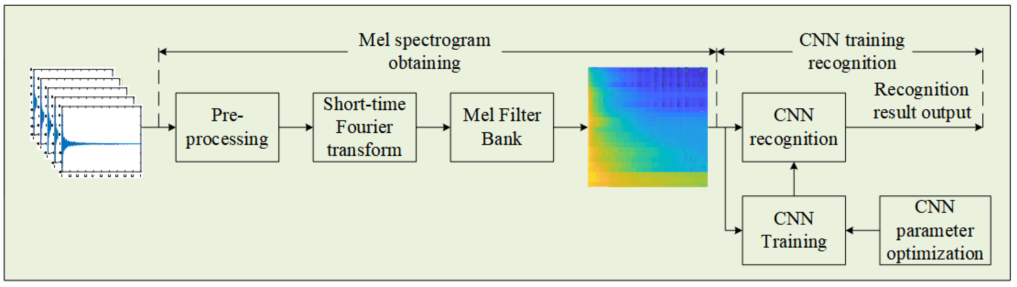
2.1. Working Principle

The flowchart of the proposed method is presented in Figure 1. In general, it consists of three steps: percussion signal acquisition, signal processing, and automatic pattern recognition based on the CNN. In the first step, the acoustic signal generated by the percussion on the pipeline with different ponding volumes was recorded by a microphone, where six ponding volumes were considered. The signal processing step included three consecutive processing stages: preprocessing, STFT method, and Mel filtering. Pre-processing was applied to the percussion signal to delete any low-frequency interference components in the sound signal, and to increase the proportion of high-frequency components. Then, using both overlap and a Hamming window, the STFT was used to obtain the time–frequency plane of the current signal. Finally, the Mel filtering was applied to the frequency axis after the STFT to obtain the Mel spectrogram with lower dimensions by compressing the frequency range, which made the CNN less computationally intensive. In the pattern recognition step, a CNN is proposed to classify the ponding volume case in an automatic way. It is worth noting that the time–frequency plane obtained through the Mel spectrogram was treated as an image in order to implement a conventional two-dimensional (2D) CNN. In the 2D CNN design, learning rates, batch sizes, and dataset split ratios were analyzed.

2.2. Mel Spectrogram
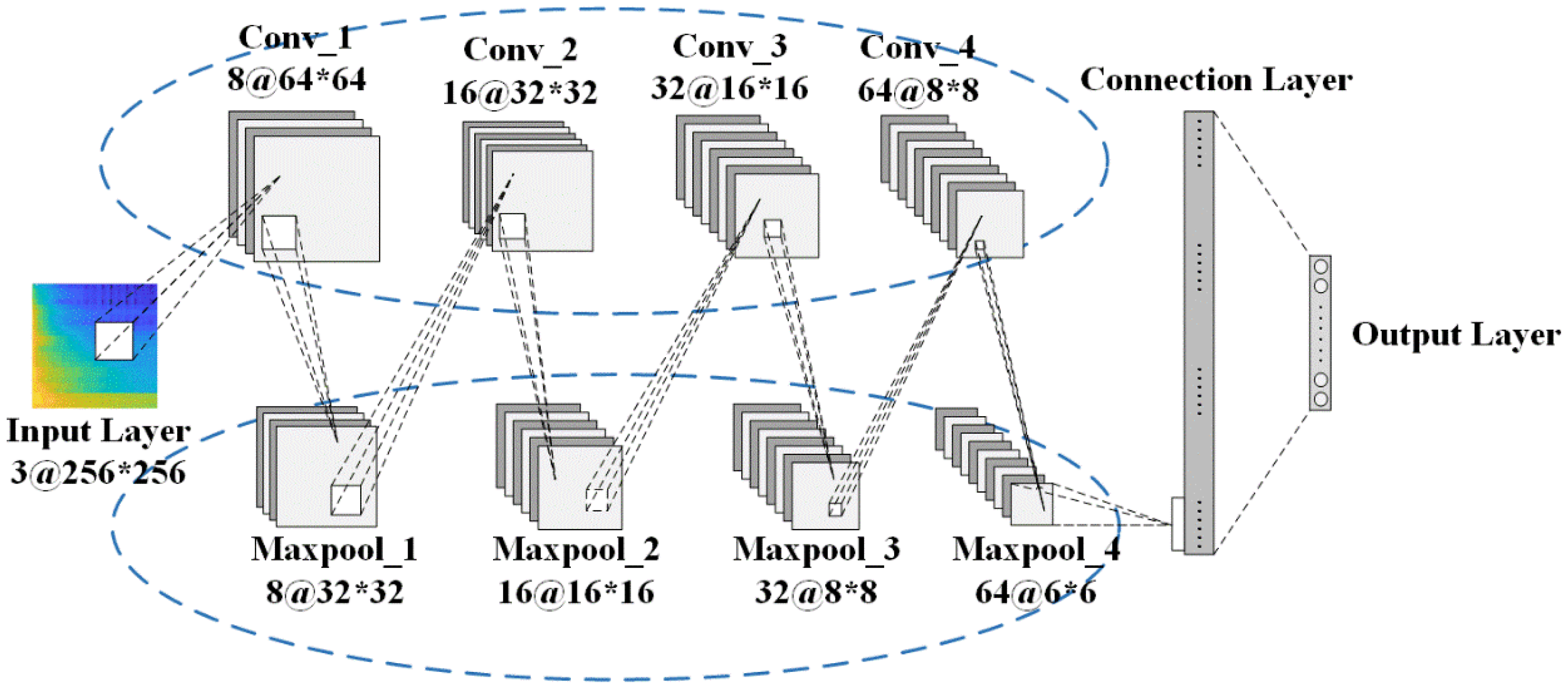
The Mel spectrogram is obtained with the following procedures:
I: Perform pre-processing of the selected signal including pre-emphasis, framing and windowing;
II: Perform short-time Fourier transform of the pre-processed data;
III: Perform Mel filtering of the data after step II to obtain the Mel spectrogram.

2.3. CNN

The recognition process of the convolutional model can be divided into two parts: CNN training and CNN recognition. In the training process of CNNs, the model parameters and training steps are preset; then, the model parameters are continuously corrected through the data forward propagation process, and error backward propagation process, until the convolutional model meets the requirements. In the CNN recognition, the high-dimensional features extracted by convolution and pooling operations are matched with the trained model to output recognition results.
The structure of the CNN model proposed in this paper is shown in Figure 2. It consists of four nonlinear trainable convolutional layers, four nonlinear fixed convolutional layers (Pooling Layer) and one fully connected layer.
Among them, the role of the convolutional layer was to perform adaptive feature extraction on the Mel spectrogram, which was achieved by convolutional operations of the convolutional kernel matrix [34]. The operation of the convolutional layer is as follows:
C l = x = 1 m y = 1 n z = 1 p a x , y , z ω x , y , z l + b l , l = 1 , 2 , , q
where l is the convolutional kernel number, Cl is the lth layer feature map of CNN, a is the input of convolutional layer, ω is the weight matrix, b is the bias term of convolutional kernel, and x, y, z are the different dimensions of the input data.
Adding a pooling layer after the convolution layer allows downsampling of the input features while preserving the dominant features, which can reduce the model parameters at the same time as suppressing overfitting [35]. The CNN model proposed in this paper uses maximum value pooling, and its expression is:
G l = d o w n s a m p ( H l ) = max H l ( v 1 , v 2 )
where Hl is the pooling layer input feature, Gl is the pooling layer output feature, and (v1, v2) is the classification element that is pooled for the previous layer.
After the Mel spectrum is propagated through several convolutional and pooling layers alternately, the fully connected layer network is relied upon to classify the extracted features, and its expression is:
h l = f ( W l h l 1 + b l )
where hl−1 is the output of the previous network layer, hl is the output of the current fully connected layer, Wl is the weight, bl is the bias, and f(*) is the activation function.

2.4. CNN Model Evaluation Metrics

The performance of the final trained CNN model needed to be evaluated by corresponding metrics [36]. Common evaluation metrics for classification tasks are Precision, Recall, and F1-Measure [37,38], which have the following equations:
P = T P T P + F P
R = T P T P + F N
F 1 = 2 P R P + R
where TP indicates a positive sample is correctly identified as a positive sample, TN indicates a negative sample is correctly identified as a negative sample, FP indicates a false positive sample (which means a negative sample is incorrectly identified as a positive sample), and FN indicates a false negative sample (which means a positive sample is incorrectly identified as a negative sample).

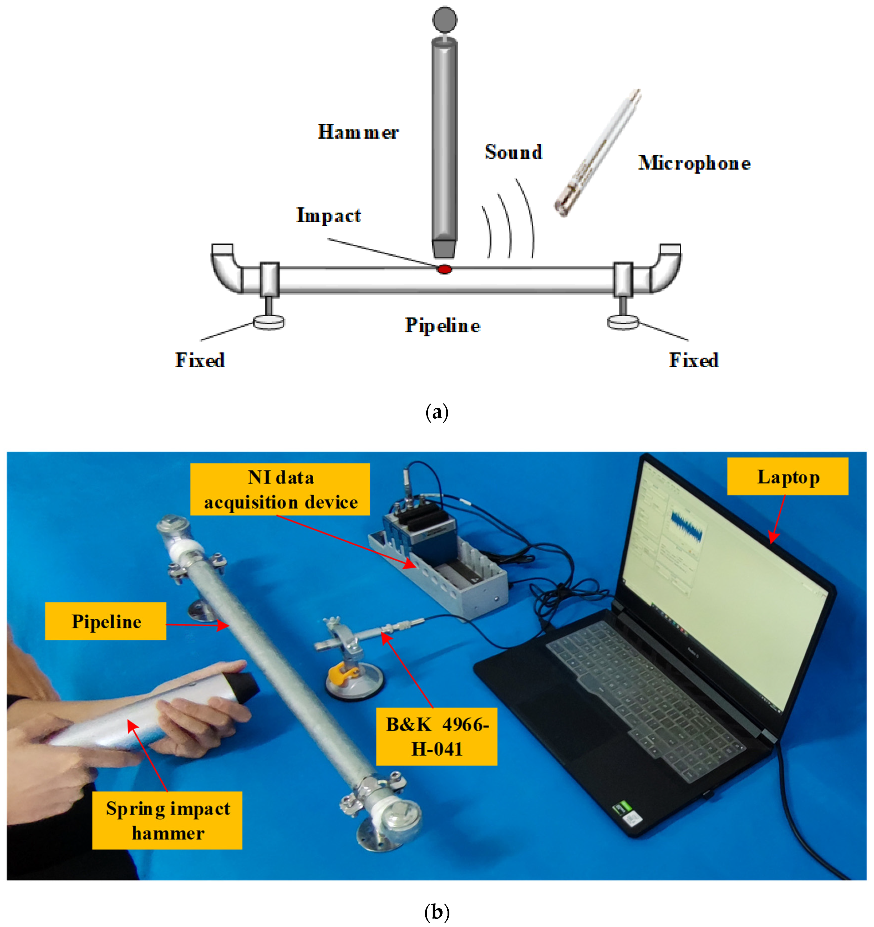
3. Experimental Setup and Procedures

As shown in Figure 3, the pipeline was fixed by a holding device, a spring-loaded impact hammer applied an impact on the middle position of the pipeline, and a microphone with a frequency band of 10 Hz~20 kHz was placed about 5 cm away from the impact position to capture the percussive acoustic signal generated by the impact. During the experiments, the sampling rate of the data acquisition device was set to 100 kHz.
In the tests, six pipelines specimens with different dimensions were fabricated; the dimensions of these specimens are listed in Table 1.
During the test, to simulate different ponding states of the pipelines, the specimens were filled with different volume percentages of water. There were a total of six experimental cases, which are listed in Table 2. The energy of each impact of the spring-loaded hammer was constant at 1J. Only the selected signal was filtered with a band-pass filter matching the microphone frequency, and 100 experiments were performed for each case.

4. Experimental Results

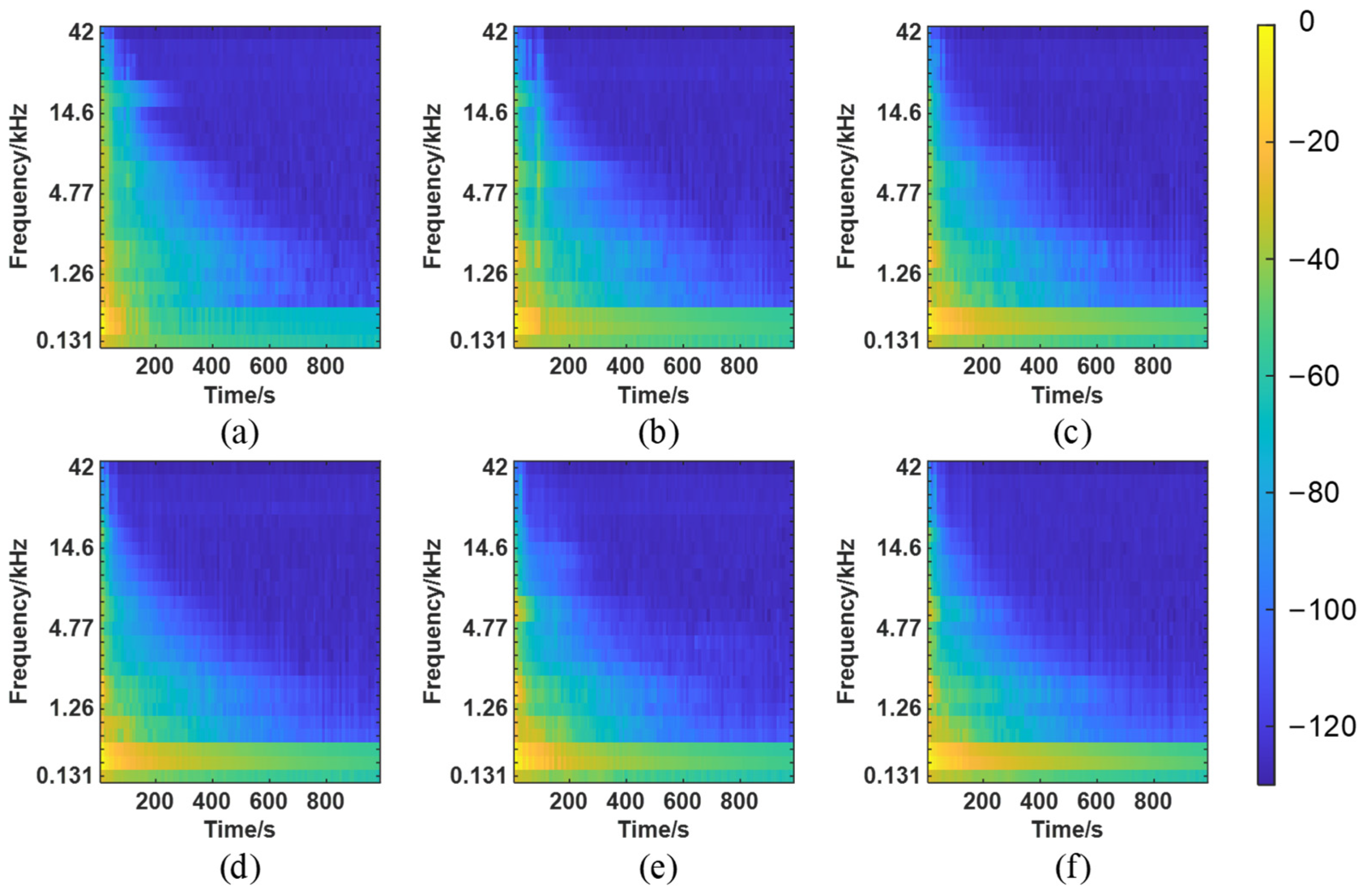
4.1. Mel-Feature Extraction

The typical percussive sound signals of the pipeline with experimental cases are shown in Figure 4.
The filtered signals were then converted into a Mel spectrogram and the parameters [39,40] were set, as shown in Table 3. The extracted Mel spectrogram features are shown in Figure 5. The results show that the differences in the Mel spectrogram of the six ponding volumes of the 1#pipeline are very small and difficult to distinguish with the naked eye.

4.2. Identification of the Amount of Ponding Volume in a Single Pipeline

Before the CNN is trained, a finer selection of other parameters such as learning rate and batch size can be carried out. The learning rate determines the step size of adjusting weights and error reduction in the training process. Figure 6 shows the obtained results for different learning rates by considering only one epoch. One epoch is a complete pass over the entire dataset. The results demonstrate that extreme values have a negative impact on accuracy. Therefore, in this work, a learning rate value of 0.01 was used, as it presented a higher accuracy and accelerated the error convergence. Table 4 shows the results of accuracy and computation time obtained using different values of batch size. The batch size determines the size of the subset of the entire dataset used in each training iteration. As indicated in Table 4, a small batch size value generates high accuracy, but results in a high computation time. On the contrary, a high value of batch size reduces the computational time, but the accuracy is negatively affected. In this regard, we chose a batch size of 30 because it provided high accuracy and a suitable computational time. Additionally, SGDM was used as the optimizer and ReLU was used as the activation function.
After we selected the above-mentioned parameters, the CNN could be completely trained and validated. However, before using the dataset to train the model, the whole dataset needed to be divided into a training set and a validation set. With the dataset well partitioned, the speed of model applications can be improved. If the partitioning is not good, it can greatly affect the deployment of the model applications. Table 5 shows the results of accuracy and computation time obtained using different ratios of dataset split. This table demonstrates that the CNN model has the highest accuracy and its application speed is optimal when the dataset splitting ratio is 7:3. Therefore, in the training process of the convolutional model, 70 sets of data obtained under each experimental case were randomly selected and converted into the Mel spectrogram, then input into the CNN as the training set. The remaining 30 sets were input into the trained CNN model as validation sets to complete the recognition of the pipeline ponding volume.
The training process of the CNN model for six ponding volume cases in the 1#pipeline is shown in Figure 7, and the recognition results are shown in Table 6.
Figure 7a shows that, with the increase in training times, the accuracy rate increases alternately and its fluctuation is large; after the number of training times reaches 146, the accuracy rate reaches 98.34%. Figure 7b indicates that the value of the loss function decreases continuously with the increase in training times, and finally stabilizes at about 0.086. Table 6 shows the CNN predictions for different case validation sets, and it can be calculated that the accuracies are 96.67%, 100%, 100%, 96.67%, 100% and 96.67%, respectively. The results show that the proposed approach can classify different ponding volume cases with high accuracy.

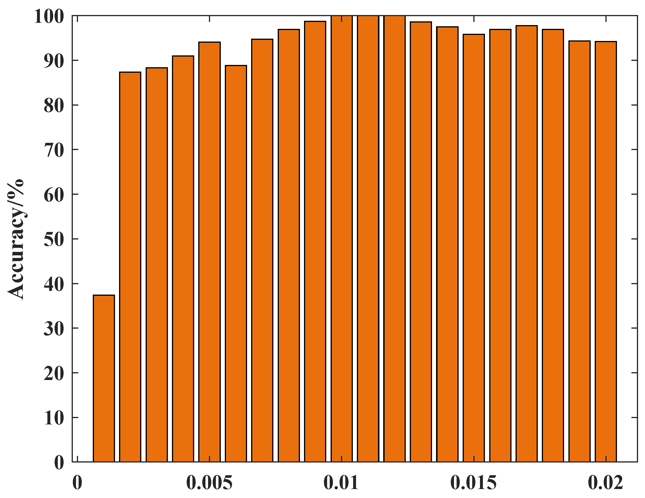
4.3. The CNN Model Evaluation of Ponding Volume in Different Pipelines

Based on the proposed method, the recognition of ponding volume for different pipelines was also performed. The three common evaluation metrics of Precision (P), Recall (R), and F1-Measure (F1) in the classification task were chosen to evaluate the final trained CNN model, as shown in Table 7.
Table 7 demonstrates that the output performance of the six pipeline CNN models is an accuracy rate of 90.9–100%, a recall rate of 90–100%, and an F1-Measure of 94.7–100%. The results show the proposed approach is effective and the evaluation results can accurately classify the ponding volume in different pipelines.

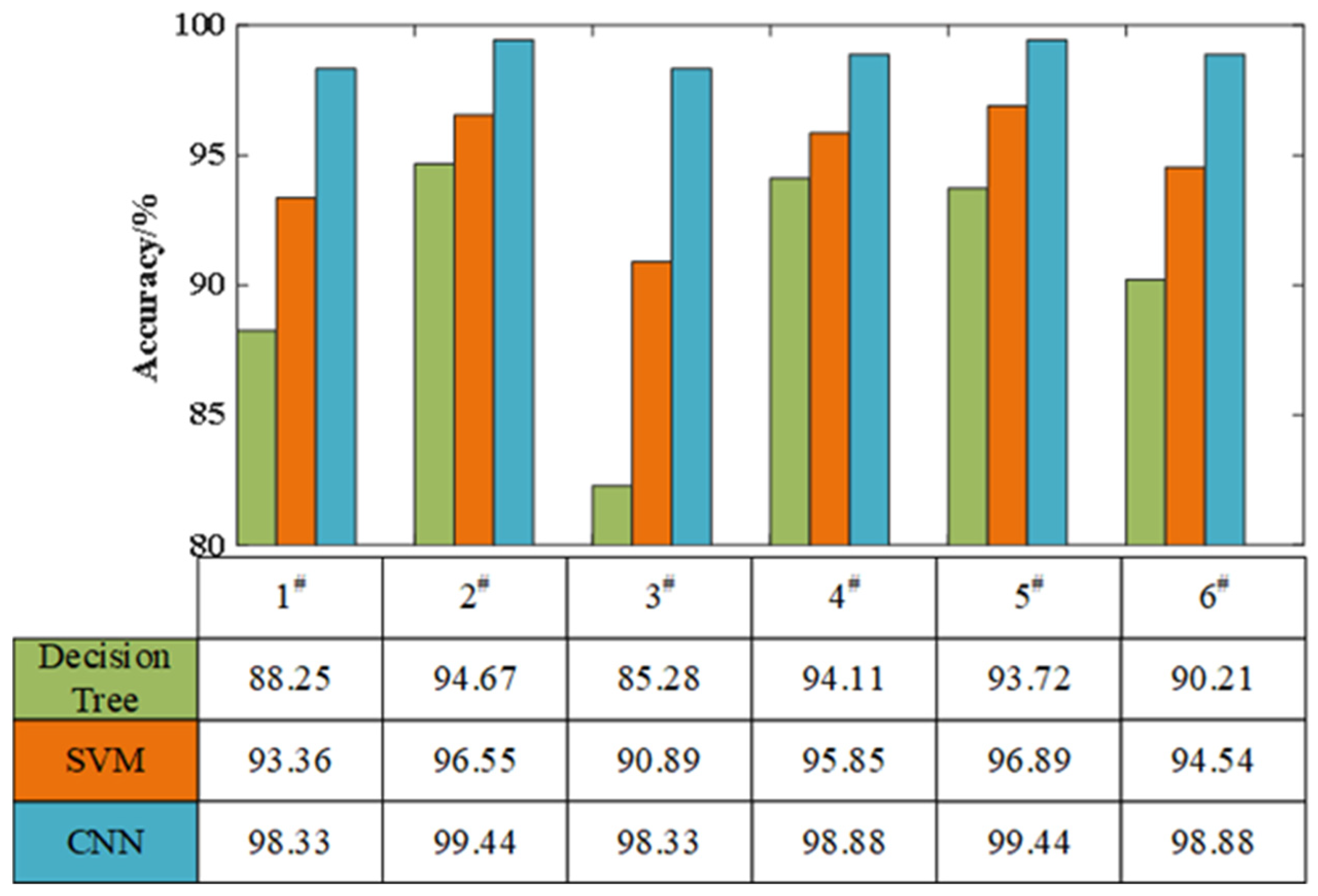
4.4. Comparison of Proposed CNN Model with Other Models

To compare the proposed method with the current common methods, experiments of identical strategies but using DTM and SVM were conducted, with the Mel spectrogram as the input image. The SVM process was performed with the LIBSVM toolbox [41], with RBF as the kernel function and a kernel function with a parameter coefficient g of 2−27, and a penalty factor coefficient c of 26 [22]. The DTM utilized the TreeBagger function, and NumTrees is set to 50 [42]. These recognition results are shown in Figure 8.
In Figure 8, the symbols of 1#, 2#, 3#, 4#, 5#, 6# denote six different pipelines as shown in Table 1, respectively. This figure highlights that the recognition accuracies of the DTM with ponding volume of six pipelines are between 88.25% and 94.67%, the recognition accuracies of the SVM between 90.89% and 96.89%, and the recognition accuracies of the CNN between 98.33% and 99.44%. This proves that the CNN recognition model is more stable and has a higher accuracy than the other two models.

5. Conclusions

The paper has proposed a novel approach to identifying pipeline ponding volumes, by combining the percussive detection method and a CNN. The proposed approach is low-cost but user-friendly and effective. The experiment was performed based on the proposed method and the experimental results show the effectivity and high accuracy of the proposed recognition model. The major findings of the proposed approach can be summarized as follows:
  • The way of processing percussion-caused audio signal by converting to Mel spectrogram can be considered as a novel and cost-effective approach in detecting pipeline ponding volume. It presents a simple but very effective acoustic signal processing method;
  • The actual output of the CNN is basically consistent with the theoretical output during the proposed approach. The results demonstrate that the CNN recognition accuracy reaches 98.34% and can be effectively adopted to pipeline ponding detection;
  • The proposed method is suitable for the detection of ponding volume in pipelines of different specifications, and the output performance of the six pipelines in the CNN models had an accuracy rate of 90.9–100%, a recall rate of 90–100%, and an F1-Measure of 94.7–100%;
  • The recognition accuracy of CNN falls between 98.33% and 99.44%, which indicates that this recognition model has a more stable and superior performance than the DTM recognition model and the SVM recognition model. Therefore, it can be concluded that the method combining the percussive detection method and the CNN proposed in this paper has better application prospects in pipeline ponding detection.
The research in this paper demonstrates the feasibility and effectiveness of the proposed pipeline ponding detection method. The essence and mechanism of the proposed method is identifying underlying dynamical characteristics of percussion-caused audio signals of pipeline ponding. However, this paper also has its shortcomings: the length and diameter of the six different pipelines selected were too singular to determine the effective detection distance of the proposed percussion detection method. In follow-up research, designing corresponding experiments to detect the effective distance of the percussive detection method in pipeline health detection will become our research focus.

Author Contributions

Conceptualization, D.Y.; Data curation, M.X.; Funding acquisition, G.L.; Investigation, M.X.; Methodology, D.Y.; Project administration, M.X.; Resources, D.Y.; Software, M.X.; Supervision, D.Y. and T.W.; Validation, M.X.; Writing—original draft preparation, M.X.; Writing—review and editing, T.W. and G.L. All authors have read and agreed to the published version of the manuscript.

Funding

This research was funded by National Natural Science Foundation of China (Grant No.: 51808417).

Institutional Review Board Statement

Not applicable.

Informed Consent Statement

Not applicable.

Data Availability Statement

Due to the nature of this research, participants of this study did not agree for their data to be shared publicly and only available upon reasonable request.

Conflicts of Interest

The authors declare no conflict of interest.

References

  1. Zhang, J.; Wang, Z.; Liu, S.; Zhang, W.; Yu, J.; Sun, B. Prediction of hydrate deposition in pipelines to improve gas transportation efficiency and safety. Appl. Energy 2019, 253, 113521. [Google Scholar] [CrossRef]
  2. Zhu, Y.; Wang, P.; Wang, Y.; Tong, R.; Yu, B.; Qu, Z. Assessment method for gas supply reliability of natural gas pipeline networks considering failure and repair. J. Nat. Gas Sci. Eng. 2021, 88, 103817. [Google Scholar] [CrossRef]
  3. Huh, C.; Kang, S.G.; Cho, M.I.; Baek, J.H. Effect of Water and Nitrogen Impurities on CO2 Pipeline Transport for Geological Storage. Energy Procedia 2011, 4, 2214–2221. [Google Scholar] [CrossRef] [Green Version]
  4. Chae, M.; Jeong, H.D. Acceptance Sampling Plans for Pipeline Condition Assessment. J. Pipeline Syst. Eng. Pract. 2019, 10, 04019024. [Google Scholar] [CrossRef]
  5. Zeng, W.; Dang, X.; Li, S.; Wang, H.; Wang, H.; Wang, B. Application of non-contact magnetic corresponding on the detection for natural gas pipeline. E3S Web Conf. 2020, 185, 01090. [Google Scholar] [CrossRef]
  6. Licata, M.; Parker, H.M.O.; Aspinall, M.D.; Bandala, M.; Cave, F.; Conway, S.; Gerta, D.; Joyce, M.J. Fast neutron and γ-ray backscatter radiography for the characterization of corrosion-born defects in oil pipelines. Eur. Phys. J. Conf. 2020, 225, 06009. [Google Scholar] [CrossRef]
  7. Soltysik, R.C. CCTV Pipeline Inspection System Data Management System and Computer-Based Monitoring/Action Application. U.S. Patent 7916170, 29 March 2011. [Google Scholar]
  8. Khan, M.S. An acoustic based approach for mitigating sewer system overflows. In Proceedings of the Global Humanitarian Technology Conference, Seattle, DC, USA, 13–16 October 2016; pp. 782–789. [Google Scholar]
  9. Hemavathi, R.; Pushpalatha, B.A. Crack and Object Detection in Pipeline using Inspection Robot. J. Trend Sci. Res. Dev. 2018, 2, 1072–1077. [Google Scholar]
  10. Wang, T.; Wei, D.; Shao, J.; Li, Y.; Song, G. Structural Stress Monitoring Based on Piezoelectric Impedance Frequency Shift. J. Aerosp. Eng. 2018, 31, 04018092. [Google Scholar] [CrossRef]
  11. Mustapha, S. Ultrasonic method for Measuring transport parameters using only the reflected waves at the first interface of porous materials having a rigid frame. INTER—NOISE NOISE—CON Congr. Conf. Proc. 2016, 253, 7258–7263. [Google Scholar]
  12. Finger, C.; Saydak, L.; Vu, G.; Timothy, J.J.; Meschke, G.; Saenger, E.H. Sensitivity of Ultrasonic Coda Wave Interferometry to Material Damage—Observations from a Virtual Concrete Lab. Materials 2021, 14, 4033. [Google Scholar] [CrossRef]
  13. Zheng, G.; Tian, Y.; Zhao, W.; Jia, S.; He, N. Band-Stop Filtering Method of Combining Functions of Butterworth and Hann Windows to Ultrasonic Guided Wave. J. Pipeline Syst. Eng. Pract. 2022, 13, 04021076. [Google Scholar] [CrossRef]
  14. Yu, Y.; Safari, A.; Niu, X.; Drinkwater, B.; Horoshenkov, K.V. Acoustic and ultrasonic techniques for defect detection and condition monitoring in water and sewerage pipes: A review. Appl. Acoust. 2021, 183, 108282. [Google Scholar] [CrossRef]
  15. Saracino, G.; Ambrosino, F.; Bonechi, L.; Cimmino, L.; D’Alessandro, R.; D’Errico, M.; Noli, P.; Scognamiglio, L.; Strolin, P. Applications of muon absorption radiography to the fields of archaeology and civil engineering. Philos. Trans. Ser. A Math. Phys. Eng. Sci. 2018, 377, 20180057. [Google Scholar] [CrossRef] [Green Version]
  16. Yao, M.; Duvauchelle, P.; Kaftandjian, V.; Peterzol-Parmentier, A.; Schumm, A. Simulation of Computed Radiography X-ray Imaging Chain Dedicated to Complex Shape Objects. Eur. Conf. Non Destr. Test. 2014, 10, 6–10. [Google Scholar]
  17. Schulze, R.; Krummenauer, F.; Schalldach, F.; d’Hoedt, B. Precision and accuracy of measurements in digital panoramic radiography. Dento Maxillo Facial Radiol. 2000, 29, 52–56. [Google Scholar] [CrossRef]
  18. Ju, F.H.; Gong, X.B.; Jiang, L.B.; Hong, H.H.; Yang, J.C.; Xu, T.Z.; Chen, Y.; Wang, Z. Chronic myeloid leukaemia following repeated exposure to chest radiography and computed tomography in a patient with pneumothorax: A case report and literature review. Oncol. Lett. 2016, 11, 2398–2402. [Google Scholar] [CrossRef] [Green Version]
  19. Adams, R.D.; Cawley, P.; Pye, C.J.; Stone, B.J. A vibration technique for non-destructively assessing the integrity of structures. J. Mech. Eng. Sci. 1978, 20, 93–100. [Google Scholar] [CrossRef]
  20. Cawley, P.; Adams, R.D. The mechanics of the coin—tap method of nondestructive testing. J. Sound Vib. 1988, 122, 299–316. [Google Scholar] [CrossRef]
  21. Cawley, P.; Adams, R.D. Sensitivity of the coin—tap method of nonde-structive testing. Mater. Eval. 1989, 47, 558–563. [Google Scholar]
  22. Kong, Q.; Zhu, J.; Ho SC, M.; Song, G. Tapping and listening: A new approach to bolt looseness monitoring. Smart Mater. Struct. 2018, 27, 07LT02. [Google Scholar] [CrossRef]
  23. Adams, R.D. Vibration measurements in nondestructive testing. In Proceedings of the 3rd International Conference on Emerging Technologies in Non Destructive Testing, Thessaloniki, Greece, 26–28 May 2003; pp. 27–35. [Google Scholar]
  24. Wang, F.; Song, G. A novel percussion-based method for multi-bolt looseness detection using one-dimensional memory augmented convolutional long short-term memory networks. Mech. Syst. Signal Process. 2021, 161, 107955. [Google Scholar] [CrossRef]
  25. Wang, F.; Ho, S.; Song, G. Modeling and analysis of an impact-acoustic method for bolt looseness identification. Mech. Syst. Signal Processing 2019, 133, 106249. [Google Scholar] [CrossRef]
  26. Zheng, L.; Cheng, H.; Huo, L.; Song, G. Monitor concrete moisture level using percussion and machine learning. Constr. Build. Mater. 2019, 229, 117077. [Google Scholar] [CrossRef]
  27. Chen, D.; Montano, V.; Huo, L.; Fan, S.; Song, G. Detection of subsurface voids in concrete-filled steel tubular (CFST) structure using percussion approach. Constr. Build. Mater. 2020, 262, 119761. [Google Scholar] [CrossRef]
  28. Lall, A.; Scalzo, F.; Ullman, H.; Liebeskind, D.S.; Chien, A. Abstract P494: Automatically Predicting Modified Treatment in Cerebral Ischemia Scores From Patient Digital Subtraction Angiography Using Deep Learning. Stroke 2021, 52 (Suppl. 1), AP494. [Google Scholar] [CrossRef]
  29. Sharif Razavian, A.; Azizpour, H.; Sullivan, J.; Carlsson, S. CNN Features off-the-shelf: An Astounding Baseline for Recognition. In Proceedings of the 2014 IEEE Conference on Computer Vision and Pattern Recognition Workshops, Columbus, OH, USA, 23–28 June 2014; pp. 806–813. [Google Scholar]
  30. Permana, S.D.H.; Saputra, G.; Arifitama, B.; Caesarendra, W.; Rahim, R. Classification of Bird Sounds as an Early Warning Method of Forest Fires using Convolutional Neural Network (CNN) Algorithm. J. King Saud Univ.—Comput. Inf. Sci. 2021; in press. [Google Scholar] [CrossRef]
  31. Hidayat, A.A.; Cenggoro, T.W.; Pardamean, B. Convolutional Neural Networks for Scops Owl Sound Classification. Procedia Comput. Sci. 2021, 179, 81–87. [Google Scholar] [CrossRef]
  32. Valtierra-Rodriguez, M.; Rivera-Guillen, J.R.; Basurto-Hurtado, J.A.; De-Santiago-Perez, J.J.; Granados-Lieberman, D.; Amezquita-Sanchez, J.P. Convolutional Neural Network and Motor Current Signature Analysis during the Transient State for Detection of Broken Rotor Bars in Induction Motors. Sensors 2020, 20, 3721. [Google Scholar] [CrossRef]
  33. Liu, F.; Shen, T.; Luo, Z.; Zhao, D.; Guo, S. Underwater target recognition using convolutional recurrent neural networks with 3-D Mel-spectrogram and data augmentation. Appl. Acoust. 2021, 178, 107989. [Google Scholar] [CrossRef]
  34. Xie, J.; Hu, K.; Guo, Y.; Zhu, Q.; Yu, J. On loss functions and CNNs for improved bioacoustic signal classification. Ecol. Inform. 2021, 64, 101331. [Google Scholar] [CrossRef]
  35. Alzubaidi, L.; Zhang, J.; Humaidi, A.J.; Al Dujaili, A.; Duan, Y.; Al Shamma, O.; Santamaría, J.; Fadhel, M.A.; Al Amidie, M.; Farhan, L. Review of deep learning: Concepts, CNN architectures, challenges, applications, future directions. J. Big Data 2021, 8, 53. [Google Scholar] [CrossRef]
  36. Rodríguez-González, A.; Torres-Niño, J.; Valencia-Garcia, R.; Mayer, M.A.; Alor-Hernandez, G. Using experts feedback in clinical case resolution and arbitration as accuracy diagnosis methodology. Comput. Biol. Med. 2013, 43, 975–986. [Google Scholar] [CrossRef]
  37. Manochandar, S.; Punniyamoorthy, M. A new user similarity measure in a new prediction model for collaborative filtering. Appl. Intell. 2020, 5, 586–615. [Google Scholar] [CrossRef]
  38. Yan, L.; Zhong, B.; Ma, K.K. Confusion-Aware Convolutional Neural Network for Image Classification. In Proceedings of the International Conference on Neural Information Processing, Sydney, Australia, 12–15 December 2019. [Google Scholar]
  39. Jung, S.Y.; Liao, C.H.; Wu, Y.S.; Yuan, S.M.; Sun, C.T. Efficiently Classifying Lung Sounds through Depthwise Separable CNN Models with Fused STFT and MFCC Features. Diagnostics 2021, 11, 732. [Google Scholar] [CrossRef]
  40. Algermissen, S.; Hörnlein, M. Person Identification by Footstep Sound Using Convolutional Neural Networks. Appl. Mech. 2021, 2, 257–273. [Google Scholar] [CrossRef]
  41. Chang, C.-C.; Lin, C.-J. LIBSVM: A library for support vector machines. ACM Trans. Intel. Syst. Technol. 2011, 2, 1–27. [Google Scholar] [CrossRef]
  42. Cheng, H.; Wang, F.; Huo, L.; Song, G. Detection of sand deposition in pipeline using percussion, voice recognition, and support vector machine. Struct. Health Monit. 2020, 19, 2075–2090. [Google Scholar] [CrossRef]
Figure 1. Schematic diagram of the working principles.
Applsci 12 02127 g001
Figure 2. The CNN model.
Applsci 12 02127 g002
Figure 3. (a) Schematic of the experimental setup; (b) experimental setup.
Applsci 12 02127 g003
Figure 4. One of the sound signals recorded by the microphone.
Applsci 12 02127 g004
Figure 5. Mel spectrogram of 1#pipeline for 6 cases: (a) 0 case; (b) 1 case; (c) 2 case; (d) 3 case; (e) 4 case; (f) 5 case.
Applsci 12 02127 g005
Figure 6. Obtained accuracy for different learning rate values.
Applsci 12 02127 g006
Figure 7. The CNN model training process. (a) Accuracy (%), (b) Loss.
Applsci 12 02127 g007
Figure 8. Comparison of recognition accuracy of three models.
Applsci 12 02127 g008
Table 1. Dimensions of the pipeline specimens.
Pipeline NumberOuter Diameter/mmInner Diameter/mmLength/mm
1#Φ32Φ2560
2#Φ32Φ25100
3#Φ42Φ3560
4#Φ42Φ35100
5#Φ48Φ4160
6#Φ48Φ41100
Table 2. Different experimental cases with different volume percentage of water.
NameValue
Case012345
Water as a percentage of pipeline volume (%)01020304050
Table 3. Mel spectrogram Parameters.
NameValue
Fs/Hz100,000
WindowHamming
Window Length2048
Overlap Length1024
FFT Length4096
NumBands24
Table 4. Results for different batch size values.
NameValue
Batch size51015202530
Accuracy (%)98.5797.1498.3298.5799.32100
Time/s52926717013110494
Batch size354045505560
Accuracy (%)98.7393.1091.6784.7686.1983.24
Time/s847267655961
Batch size657075808590
Accuracy (%)81.3692.3882.1487.1487.6290.00
Time/s545548494142
Batch size95100
Accuracy (%)87.6291.43
Time/s4041
Table 5. Results of different splitting datasets.
NameCase
Dataset split ratio1:13:27:34:19:1
Accuracy (%)98.4797.8310097.5098.70
Time/s86928197129
Table 6. The CNN identification results of the 1#pipeline.
Target Class
012345
Predicted Class02900000
11300000
20030100
30002900
40000301
50000029
Total accuracy (%)98.34
Table 7. Three common evaluation metrics results of six pipeline dimensions.
1#Pipeline2#Pipeline3#Pipeline
RPF1RPF1RPF1
Case096.710098.310096.898.4100100100
110096.898.410010010010090.595.2
210096.898.41001001009010094.7
396.710098.3100100100100100100
410096.898.496.710098.3100100100
596.710098.3100100100100100100
4#Pipeline5#Pipeline6#Pipeline
RPF1RPF1RPF1
Case010096.898.4100100100100100100
1100100100100100100100100100
296.710098.3100100100100100100
310096.898.410010010096.796.796.7
410010010096.710098.396.710098.3
596.710098.310096.898.410096.898.4
Publisher’s Note: MDPI stays neutral with regard to jurisdictional claims in published maps and institutional affiliations.

