Method of Eliminating Helicopter Vibration Interference Magnetic Field with a Pair of Magnetometers

Abstract

The low-frequency electromagnetic fields and magnetic anomalies generated by ships and other underwater platforms are widely recognized as important features for ocean target detection. Low-frequency magnetic fields and anomalies are typically measured by optically pumped magnetometers installed on aircraft. However, the interference that is generated by the aircraft platform may significantly affect the detection performance. The traditional aeromagnetic compensation model has a good effect on eliminating the interference magnetic field that is caused by the carrier attitude variation. Usually, the magnetometer is fixed at the top of a long probe on the aircraft to avoid the influence from the main body in the aircraft. However, the probe is sensitive to external vibrations, and vibration-induced magnetic interference can occur in the measurements. The magnetometer is especially easily affected by the interference magnetic field, including the vibration frequency and harmonic frequency of the probe, in a moving platform, such as a helicopter. These interference fields usually have independent frequency characteristics that can be eliminated by compensation methods. In this paper, we propose a method based on the improved coherent noise suppression method with a pair of magnetometers to eliminate the effects from these magnetic field disturbances and improve the detection performance of the measurement system. The results of the flight experiment show that the method can effectively eliminate low-frequency vibration interference and improve the detection ability of weak signals from targets.

1. Introduction

The electromagnetic fields generated by naval vessels and other underwater carriers have become important signals for tracking targets of interest in marine warfare [1,2]. When ships and underwater carriers are in seawater, in addition to the influence of ferromagnetic materials (such as iron, cobalt, and nickel), the metal material in the carrier composition (such as the steel shell and copper propeller) electrochemically reacts to generate a corrosive current around the vessel [3]. In order to protect the hull from corrosion, the impressed current cathodic protection system and the sacrificial anode cathodic protection system are widely used to generate corrosion protection currents in modern ships. These currents create electro-static and magneto-static anomalies around the ships. At the same time, the corrosion current and the protection current flow from the hull to the propeller through the seawater. Then, the currents return to the hull from the propeller through various bearings and mechanical wires [4]. The loop electrical impedance periodically changes as the drive shaft rotates, causing the current flowing through the seawater to be modulated, thereby forming an extremely low-frequency electromagnetic field in the seawater and propagating outward. The signal has frequency characteristics that are consistent with the propeller rotation frequency and its harmonic frequency. To a large extent, the signals can be transmitted several kilometers away. Therefore, they are considered important signal sources for detecting underwater military targets [5].

As a significant passive detection method, aeromagnetic exploration is widely used in underwater target detection [6,7,8]. The development and updating of aeromagnetic testing technologies is often concentrated in the military field. Tracing back to World War II, the British Army started to use aircraft to carry fluxgate sensors to detect underwater submarines. With the development of high-precision magnetometers, such as optically pumped magnetometers (OPMs), aeromagnetic surveying has become one of the most important means of underwater target detection. Given that the aircraft platform affects the accuracy of OPM measurements, W.E. Tolles proposed a classical aeromagnetic compensation model in the 1940s [9,10]. Paul Leliak proposed sinusoidal maneuvers to improve compensation performance in 1961 [11]. In 1980, B.W. Leach proposed a ridge regression algorithm to solve the aeromagnetic compensation parameters, and the experimental results showed that this method performed well in improving the compensation performance [12]. In 1995, Hardwick designed an innovative three-axis aeromagnetic gradiometry flown on a fixed-wing platform [13]. Around 2005, Nelson carried out a series of experiments with an experimental flight system [14,15]. In 2011 and 2013, Gerardo Noriega proved the viability and reliability of using the standard deviation of the signal as an assessment criterion through a large number of aeromagnetic trials [16,17]. The traditional aeromagnetic compensation model has a good effect on eliminating the interference field caused by aircraft attitude changes, which are generally less than 2 Hz. For time-varying interferences with an unknown signature, Sheinker proposed an adaptive magnetic interference cancelation method by using a pair of magnetometers, which obtained good results for highly correlated interference magnetic fields [18]. However, for magnetic measurement systems with the magnetometers on a probe of a helicopter, the probe vibrates when the helicopter is flying. In this case, there is a vibration frequency and its harmonic interference field that can be captured by the magnetometers. The harmonic interference magnetic field that is caused by aircraft vibration seriously affects the detection of target signals to a large extent.

In order to eliminate the electromagnetic interference field that is produced by the vibration of the helicopter platform, in this paper, we propose an interference cancelation algorithm based on the improved coherent noise suppression (ICNS) method for a detection system with a pair of magnetometers. The test for the calibration and the survey line proved that the proposed algorithm in this paper effectively eliminated the interference field. As a consequence, the system performance for detecting the target signal was improved.

2. Traditional Aeromagnetic Compensation Model

According to the classical Tolles–Lawson (T–L) aeromagnetic compensation model, the aircraft interference field H_T(t) is a sum of the permanent magnetic field H_P(t), the induced magnetic field H_I(t), and the eddy current magnetic field H_E(t), and is expressed as the following equation:

$$H_T\left(t\right)=H_P\left(t\right)+H_I\left(t\right)+H_E\left(t\right).$$

(1)

Usually, a three-axis magnetometer is used to measure the attitude of the platform during the aeromagnetic compensation flight. The quantities T, L, and V can be used as the three component outputs of the geomagnetic field H_e(t). The cosine values of the angles between the platform and the geomagnetic field can be denoted as v₁, v₂, v₃, and they can be expressed as follows:

$$\begin{array}{l}{v}_1=T\left(t\right)/H_e\left(t\right)=T\left(t\right)/\sqrt{T{\left(t\right)}^2+L{\left(t\right)}^2+V{\left(t\right)}^2}\\ v_2=L\left(t\right)/H_e\left(t\right)=L\left(t\right)/\sqrt{T{\left(t\right)}^2+L{\left(t\right)}^2+V{\left(t\right)}^2}\\ v_3=V\left(t\right)/H_e\left(t\right)=V\left(t\right)/\sqrt{T{\left(t\right)}^2+L{\left(t\right)}^2+V{\left(t\right)}^2}\end{array}.$$

(2)

Then, the interference field H_T (t) can be displayed as follows:

$$H_T\left(t\right)=\left(\begin{array}{l}\begin{array}{l}{c}_1{v}_1+c_2{v}_2+c_3{v}_3\\ +H_e\left(t\right)\left(c_4{v}_1^2+c_5{v}_1{v}_2+c_6{v}_1{v}_3+c_7{v}_2^2+c_8{v}_2{v}_3+c_9{v}_3^2\right)\end{array}\\ +H_e\left(t\right)\left(\begin{array}{l}{c}_{10}{v}_1{v}_1{}^{\prime }+c_{11}{v}_1{v}_2{}^{\prime }+c_{12}{v}_1{v}_3{}^{\prime }+c_{13}{v}_2{v}_1{}^{\prime }+c_{14}{v}_2{v}_2{}^{\prime }\\ +c_{15}{v}_2{v}_3{}^{\prime }+c_{16}{v}_3{v}_1{}^{\prime }+c_{17}{v}_3{v}_2{}^{\prime }+c_{18}{v}_3{v}_3{}^{\prime }\end{array}\right)\end{array}\right)={\displaystyle {\displaystyle \sum }_{i=1}^{18}{A}_i\left(t\right)c_i}.$$

(3)

where the coefficients c_i, I = 1,2, …, 18 represent the compensation parameter, and the time-varying quantities A_i (t), I = 1, 2, …, 18 can be calculated from v₁, v₂, and v₃ and their derivatives v₁′, v₂′, and v₃′.

Since the equations v₁² + v₂² + v₃² = 1 and v₁v₁′ + v₂v₂′ + v₃v₃′ = 0, the parameters c₄, c₇, c₉, c₁₀, c₁₄, and c₁₈ are not independent. To find the stable solutions for the model, Equation (3) can be simplified by removing the items c₉v₃² and c₁₈v₃v₃′. Thus, we obtain the replaced T–L model as follows:

$$H_T\left(t\right)={\displaystyle \sum _{i=1}^{16}{A}_i\left(t\right)c_i}.$$

(4)

The corresponding matrix notation for Equation (4) can be expressed as follows:

$$\mathit{H}=\mathit{A}\mathit{C},$$

(5)

where H is the column vector constituted by the sampling points of H_T(t). C is the column vector, and it can be expressed as C = [c₁c₂…c₁₆]^T. A is the corresponding matrix constituted by the sampling points of attitude information, which can be expressed as follows:

$$A=\left[\begin{array}{cccc}{A}_1\left(1\right)& A_2\left(1\right)& \cdots & A_{16}\left(1\right)\\ A_1\left(2\right)& A_2\left(2\right)& \cdots & A_{16}\left(2\right)\\ ⋮& ⋮& \ddots & \cdots \\ A_1\left(n\right)& A_2\left(n\right)& \cdots & A_{16}\left(n\right)\end{array}\right].$$

(6)

The compensation parameters can be obtained by a least square (LS) solution that can be expressed as follows:

$$\mathit{C}={\left({\mathit{A}}^T\mathit{A}\right)}^{-1}{\mathit{A}}^T\mathit{H}.$$

(7)

Usually, after the calibration flight, the compensation coefficients can be obtained by Equation (7). Then, by taking the compensation coefficients back to Equation (5), the interference fields can be obtained and eliminated.

3. Vibration Interference Magnetic Field

The helicopter aeromagnetic system is shown in Figure 1. Two cesium OPMs (OPM-I and OPM-II) and a fluxgate magnetometer are fixedly connected to the probe. The fluxgate magnetometer is used to measure the attitude of the platform since it is vectorial. The noise performance of the OPMs is 0.6 pT/√Hz, and the fluxgate magnetometer is 6 pT/√Hz.

The design of the flight path of the calibration compensation experiment is shown in Figure 2a. The sampling rate of the recording system was 40 Hz. The helicopter flew at a height of about 3000 m to avoid interference from the ground. The compensating flight executed standard maneuvers, including a series of ±10° rolls, ±5° pitches, and ±5° yaws maneuvers along each line in the box. Figure 2 details the flight path and information.

After calculating by the LS solution, the compensation parameters of the OPM-I and OPM-II were calculated and separately listed in

Table 1. Compensation parameters of OPM-I.

Parameter	Value	Parameter	Value	Parameter	Value	Parameter	Value
c1	34.0nT	c2	5.57nT	c3	9.27nT	c4	5.61 × 105
c5	2.05 × 105	c6	4.04 × 106	c7	3.68 × 104	c8	1.78 × 104
c9	−4.96 × 105	c10	−8.73 × 105	c11	−5.31 × 106	c12	5.07 × 105
c13	−2.42 × 104	c14	−2.14 × 105	c15	−6.03 × 105	c16	−3.49 × 105

and

Table 2. Compensation parameters of OPM-II.

Parameter	Value	Parameter	Value	Parameter	Value	Parameter	Value
c1	302.7nT	c2	130.9nT	c3	−181.1nT	c4	1.59 × 104
c5	2.70 × 104	c6	−5.00 × 106	c7	3.20 × 103	c8	1.77 × 103
c9	−8.51 × 104	c10	−3.49 × 104	c11	−3.10 × 104	c12	4.51 × 104
c13	−1.53 × 103	c14	−1.37 × 103	c15	−3.31 × 104	c16	−2.91 × 104

. Consistent with the actual installation, we found that the compensation parameters of OPM-II were much larger.

Figure 3 and Figure 4 show the compensation results of the calibration flight data using the compensation parameters of Table 1 and Table 2. The blue dashed and solid lines represent the data before and after the compensation, respectively. Figure 3a and Figure 4a present the results of the processing of the compensation data through a high-pass filter with a cut-off frequency of 0.5 Hz. The signals and the noise power spectral density of the uncompensated flight data and the compensated data are shown in Figure 3b and Figure 4b, respectively. The aeromagnetic compensation had an obvious effect on the low-frequency electromagnetic interference, with a frequency below 2 Hz. Taking OPM-I as an example, the compensated interference field dropped from 45 pT/√Hz at 1 Hz to 18 pT/√Hz at 1 Hz. At higher frequencies, the traditional compensation model had essentially no effect. However, there were still many selective frequency interferences with the measurement magnetic field at 0.72 Hz, 1.445 Hz, 6.48 Hz, and so on. These multi-frequency interferences were mainly caused by the motion of the probe and the vibration interference field caused by the rotation of the propeller, which could not be eliminated by the basic aeromagnetic compensation operation.

The correlation coefficient of the residual interference magnetic field was calculated after the OPM-I and OPM-II magnetic compensation process, as shown in Figure 5. According to this figure, the correlation coefficient was high and reached or exceeded 0.8 in the fixed frequency points of the probe vibration and the rotation of the propeller, at 1.445 Hz, 2.15 Hz, 2.89 Hz, 6.48 Hz, and so on. The high correlation values indicate that the vibration interference field compensation based on the data of dual magnetometer had high feasibility to eliminate the interferences at the fixed frequencies.

4. The Proposed Method and Principle

After the aeromagnetic compensation, the interference field associated with the attitude of the aircraft was eliminated. However, the interference associated with the vibration in magnetometers was still present. These interference fields had many fixed frequency points that existed at fundamental frequencies and their harmonics. In order to eliminate the vibration interference magnetic field, we first introduced an adaptive cancelation method as a reference, and then proposed an improved coherent noise suppression (ICNS) method.

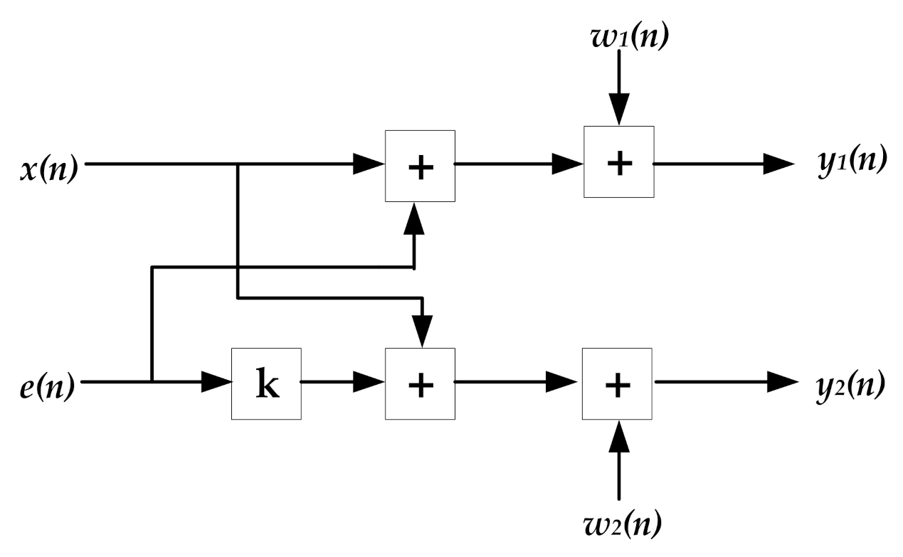
4.1. The Adaptive Interference Cancelation Method

Reference [18] introduced an adaptive method to eliminate the magnetic interference with a pair of magnetometers, and its theoretical model is shown in Figure 6, where x(n) represents the ambient magnetic field, e(n) is the magnetic interference, and w₁(n) and w₂(n) represent the intrinsic noises of OPM-I and OPM-II, respectively. The output readings of the two magnetometers are expressed as y₁(n) and y₂(n).

The model can be expressed as a set of equations, as shown in Equation (8). The interference magnetic field elimination is the solution of an adaptive coefficient k.

$$\begin{array}{l}{y}_1(n)=s(n)+e(n)+w_1\left(n\right)\\ y_2(n)=s(n)+ke(n)+w_2\left(n\right)\end{array}.$$

(8)

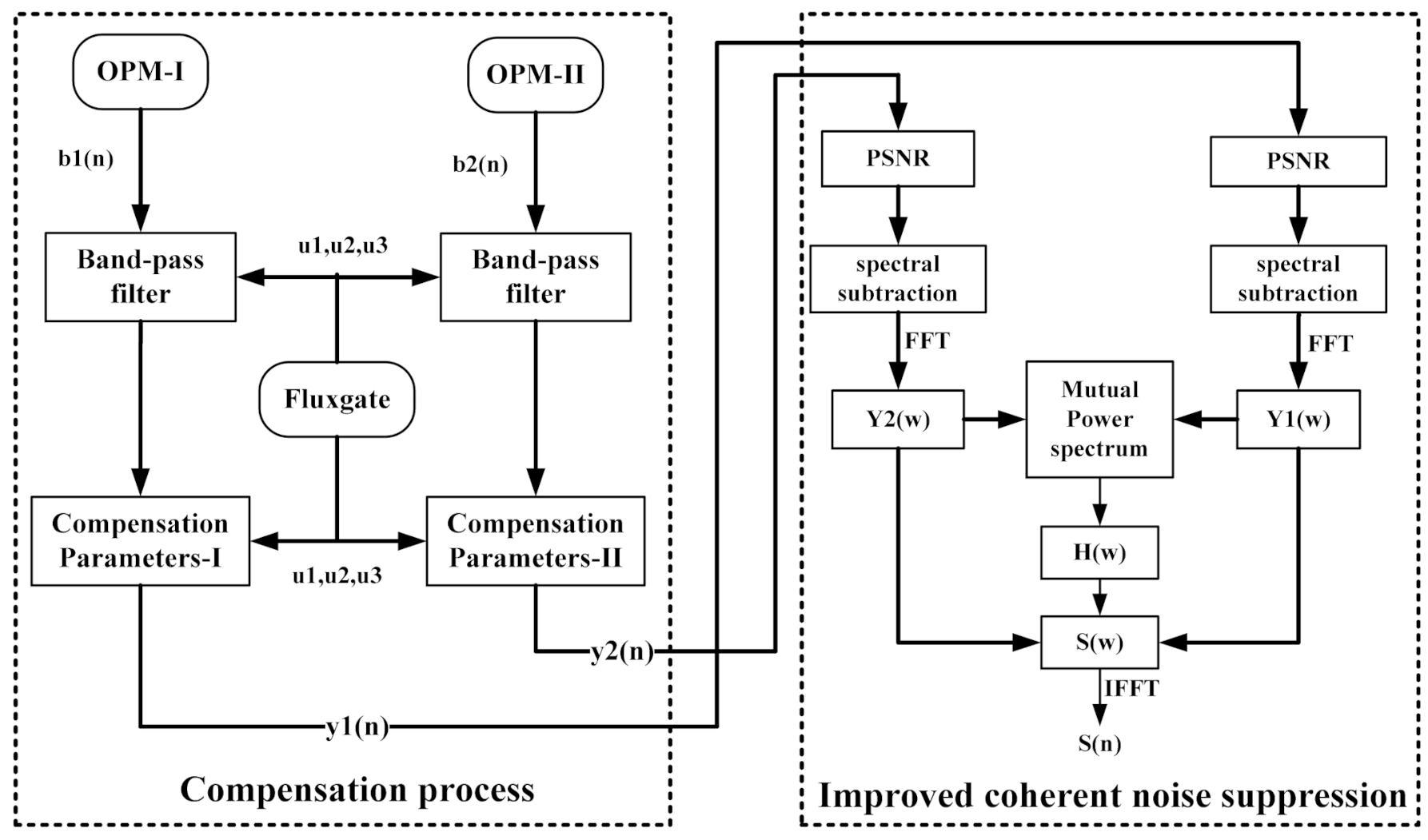
4.2. The Improved Coherent Noise Suppression (ICNS) Method

The CNS is a practical noise cancelation method. The distance between the two magnetometers is far less than the distance between the helicopter and the target, so it can be considered that the two magnetometers in the helicopter measure the common value of the magnetic field from the target and the different values from the interference field. In addition, it is known that the vibration interference field of the two magnetometers is highly correlated.

After the compensation, we obtained the magnetic field data sequences y₁(n) and y₂(n). The y₁(n) involves the signal field s(n) and interference field d(n), while y₂(n) involves the signal field s(n) and stronger interference field d₂(n). The n denotes the sample index, where w₁(n) and w₂(n) represent the intrinsic noises of OPM-I and OPM-II, respectively.

$$\begin{array}{l}{y}_1(n)=s(n)+d(n)+w_1\left(n\right)\\ y_2(n)=s(n)+d_2(n)+w_2\left(n\right)\end{array}.$$

(9)

Considering that the two magnetometers were subject to different interference levels from helicopters, the interference magnetic field that was measured by the closer magnetometer was larger and contained more interference components. In order to avoid the influence from the incoherent noise of the two magnetometers with the CNS method, it was noticed that the OPM-II had more interference field characteristics. Before the CNS processing, we needed to preprocess the measured data from the two magnetometers.

Here, we proposed a spectral subtraction method to reduce the quasi-stationary components from background interference based on a priori signal-to-noise ratio (PSNR) estimation, which was used to respectively process the measurement data from the two magnetometers. As an example, the magnetic field y₁(n) measured by OPM-I can be expressed as follows:

$$y_1(n)=s(n)+d(n)+w_1\left(n\right).$$

(10)

In the process, this signal was evenly divided into short-time frames and analyzed frame by frame, assuming that its behavior was similar over the duration of all the analyses frames. For a short time frame, k defines the spectral component of the noisy signal as Y₁(k, ω), the signal as S(k, ω), and the interference and noise as D(k, ω). The interference reduction process was used for each short-time frequency spectrum, Y₁(k, ω), with a spectral gain, G(k, ω), which is a function of two parameters in the signal-to-noise ratio with a priori, SNR_prio(k, ω), and a posteriori, SNR_post(k, ω), as shown in Equations (11)–(13).

$$SN{R}_{prio}\left(k,\omega \right)=\frac{{\left|Y_1\left(k,\omega \right)\right|}^2}{E\left\{{\left|D\left(k,\omega \right)\right|}^2\right\}}.$$

(11)

$$SN{R}_{post}\left(k,\omega \right)=\frac{{\left|S\left(k,\omega \right)\right|}^2}{E\left\{{\left|D\left(k,\omega \right)\right|}^2\right\}}.$$

(12)

$$G\left(k,\omega \right)=\sqrt{\frac{SN{R}_{prio}\left(k,\omega \right)}{SN{R}_{prio}\left(k,\omega \right)+1}}.$$

(13)

The noise power spectral density E{|D(k, ω)|²} can be estimated during the periods when the signal from the target is not present, where E is the expectation operator. The SNR_prio(k, ω) can be obtained through the following recursive relation, where α is the smoothing coefficient, which is generally a value between 0.8 and 1.

$$SN{R}_{prio}\left(k,\omega \right)=\alpha \frac{{\left|S\left(k-1,\omega \right)\right|}^2}{E\left\{{\left|D\left(k,\omega \right)\right|}^2\right\}}+\left(1-\alpha \right)\cdot max\left[SN{R}_{post}\left(k,\omega \right)-1,0\right].$$

(14)

Then, S(k, ω) is the estimated signal spectrum at the previous frame and is obtained as follows:

$$S\left(k,\omega \right)=G\left(k,\omega \right)\cdot Y_1\left(k,\omega \right).$$

(15)

After the preprocessing, the outputs of OPM-I and OPM-II can be expressed as Equations (16) and (17), where s(n), e₁(n), and e₂(n) represent the target signal, and the residual interference field in OPM-I and in OPM-II, respectively.

$$\begin{array}{l}{y}_1(n)=s(n)+e_1(n)\\ y_2(n)=s(n)+e_2(n)\end{array}.$$

(16)

By taking into account the coherence of the vibration interference field, the residual interference fields e₁(n) and e₂(n) can be expressed by Equation (17), where h(n) is the transfer function. The coherent noise suppression method regards the detector as a 2 × 2 linear time-invariant system to suppress the residual interference field from the helicopter.

$$e_2\left(n\right)=h(n)\times e_1(n).$$

(17)

By applying a discrete Fourier transform (DFT) on both sides of Equation (18), they can be represented in the frequency domain as follows:

$$\begin{array}{l}{Y}_1\left(\omega \right)=S\left(\omega \right)+E_1\left(\omega \right)\\ Y_2\left(\omega \right)=S\left(\omega \right)+E_2\left(\omega \right)=S\left(\omega \right)+H\left(\omega \right)·E_1\left(\omega \right)\end{array}.$$

(18)

Hence, the auto-spectra and cross-spectra of Y₁(ω) and Y₂(ω) are shown as Equation (19), where P_SS(ω) and P_EE(ω) are the auto-spectra of the signal and interference field, and H(ω) is the discrete Fourier transform of h(n).

$$\begin{array}{l}{P}_{Y_1{Y}_1}\left(\omega \right)=P_{SS}\left(\omega \right)+P_{EE}\left(\omega \right)\\ P_{Y_1{Y}_2}\left(\omega \right)=P_{SS}\left(\omega \right)+H^{\ast }\left(\omega \right)P_{EE}\left(\omega \right)\\ P_{Y_2{Y}_1}\left(\omega \right)=P_{SS}\left(\omega \right)+H\left(\omega \right)P_{EE}\left(\omega \right)\\ P_{Y_2{Y}_2}\left(\omega \right)=P_{SS}\left(\omega \right)+H\left(\omega \right)H^{\ast }\left(\omega \right)P_{EE}\left(\omega \right)\end{array}.$$

(19)

The transfer function H(ω) can be expressed as Equation (20). Then, the signal s(n) can be written again in a time domain by using the inverse Fourier transform, F⁻¹, as shown in Equation (21).

$$H\left(\omega \right)=\frac{P_{Y_2{Y}_2}\left(\omega \right)-P_{Y_2{Y}_1}\left(\omega \right)}{P_{Y_1{Y}_2}\left(\omega \right)-P_{Y_1{Y}_1}\left(\omega \right)}.$$

(20)

$$s\left(n\right)=F^{-1}\left(y_1\left(\omega \right)-\frac{y_2\left(\omega \right)-y_1\left(\omega \right)}{H\left(\omega \right)-1}\right).$$

(21)

Finally, the structure of the aeromagnetic compensation and the improved coherent noise suppression algorithm is shown in Figure 7, including the compensation process and the interference suppression process.

5. Results and Discussion

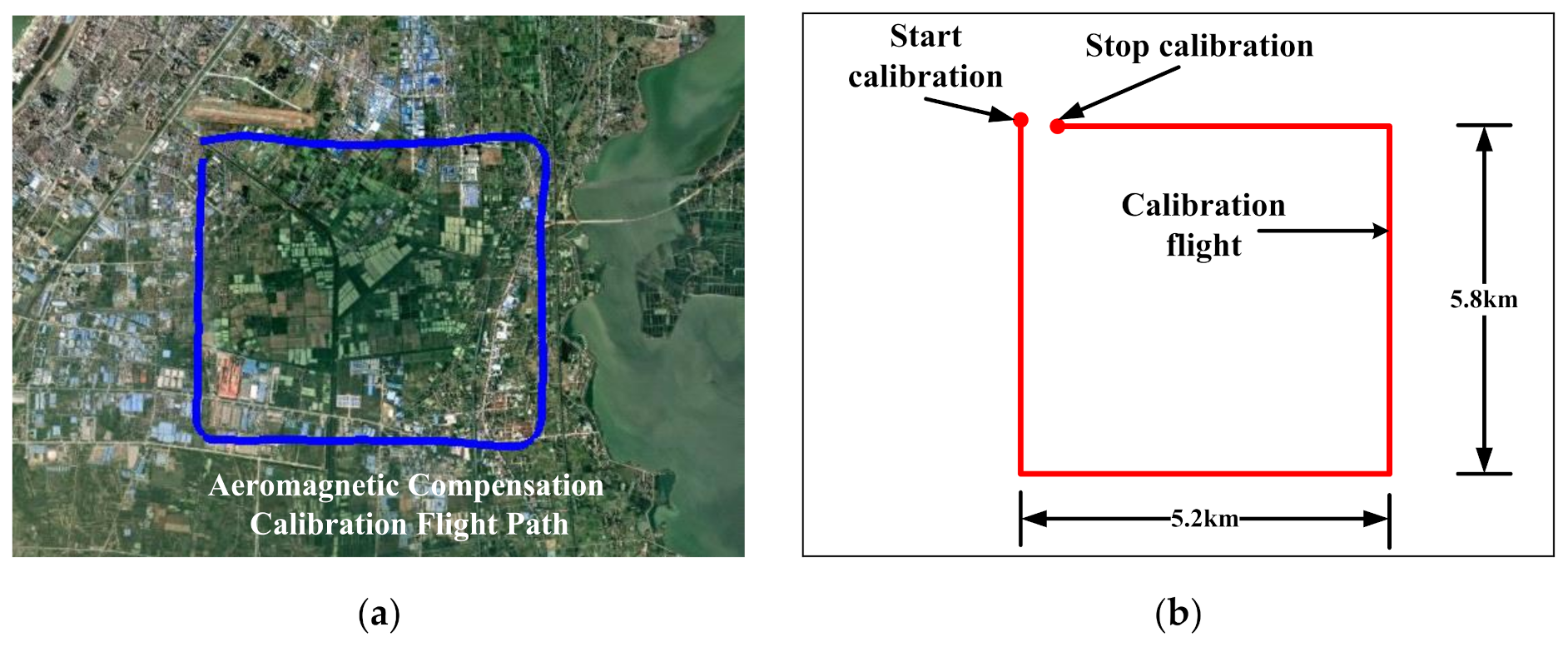
5.1. The Results of the Calibration Flight

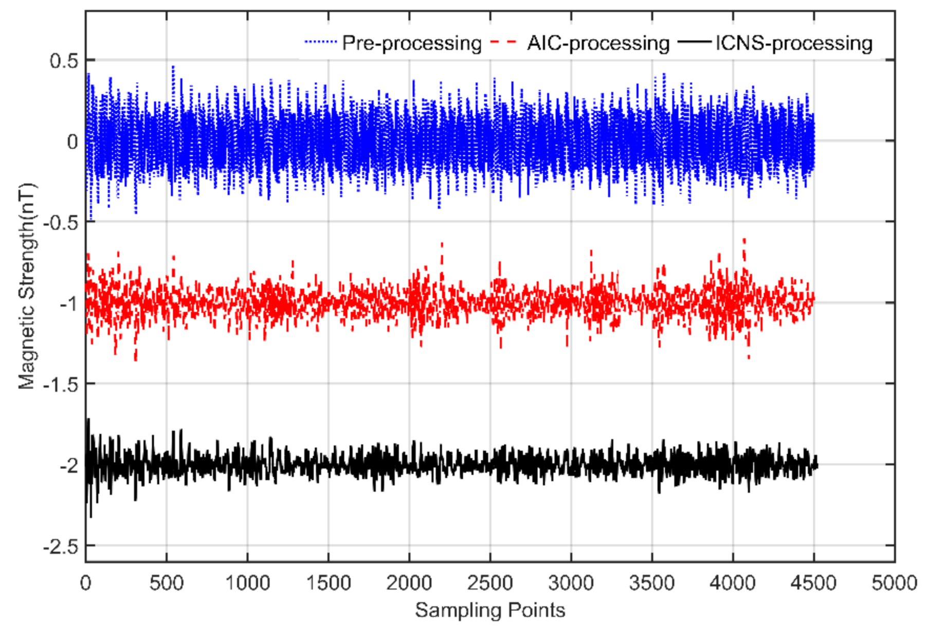
5.1.1. Results of Adaptive Interference Cancelation (AIC)

As an important reference, the AIC method is often used in advance to eliminate the vibration interference magnetic field of a helicopter, and the results are calculated by using the method shown in Figure 8. The blue dot and black solid line represent the compensated field before and after the AIC method, respectively, and the black line is a clear offset of 1nT. In Figure 8, the vibration interference magnetic field is weakened to a certain extent, after using the AIC algorithm. In order to display the effect of elimination to a more visible extent, the algorithm effect is displayed using a time–frequency diagram, as shown in Figure 9.

In Figure 9, the interference fields at multi-frequency points still exist after the proposed method. Therefore, this AIC algorithm had a very limited effect on reducing the interference that was caused by the helicopter vibration.

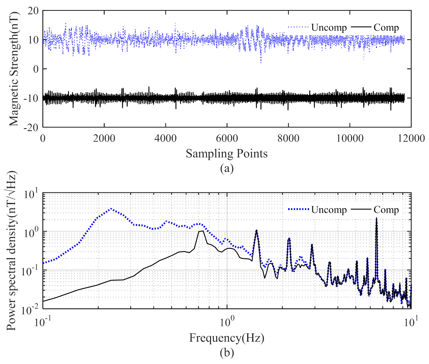
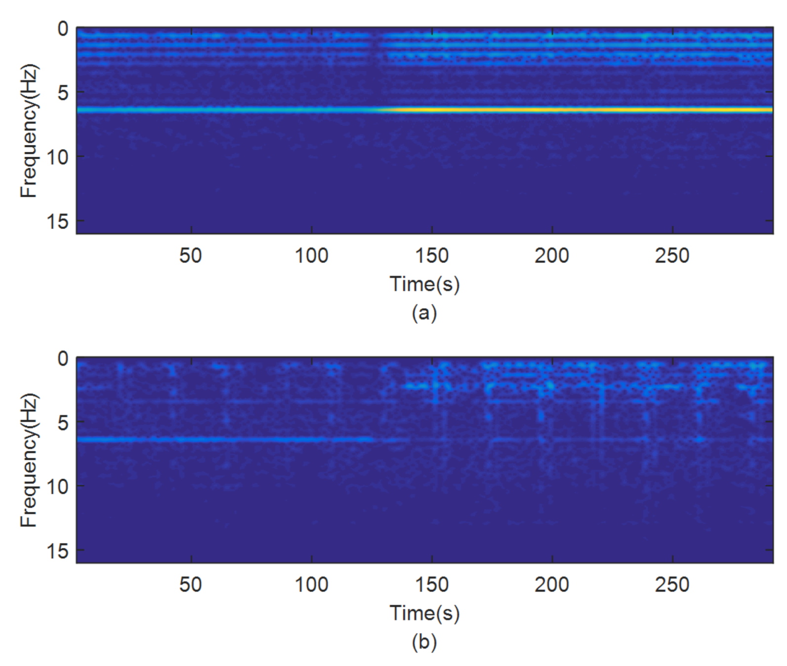
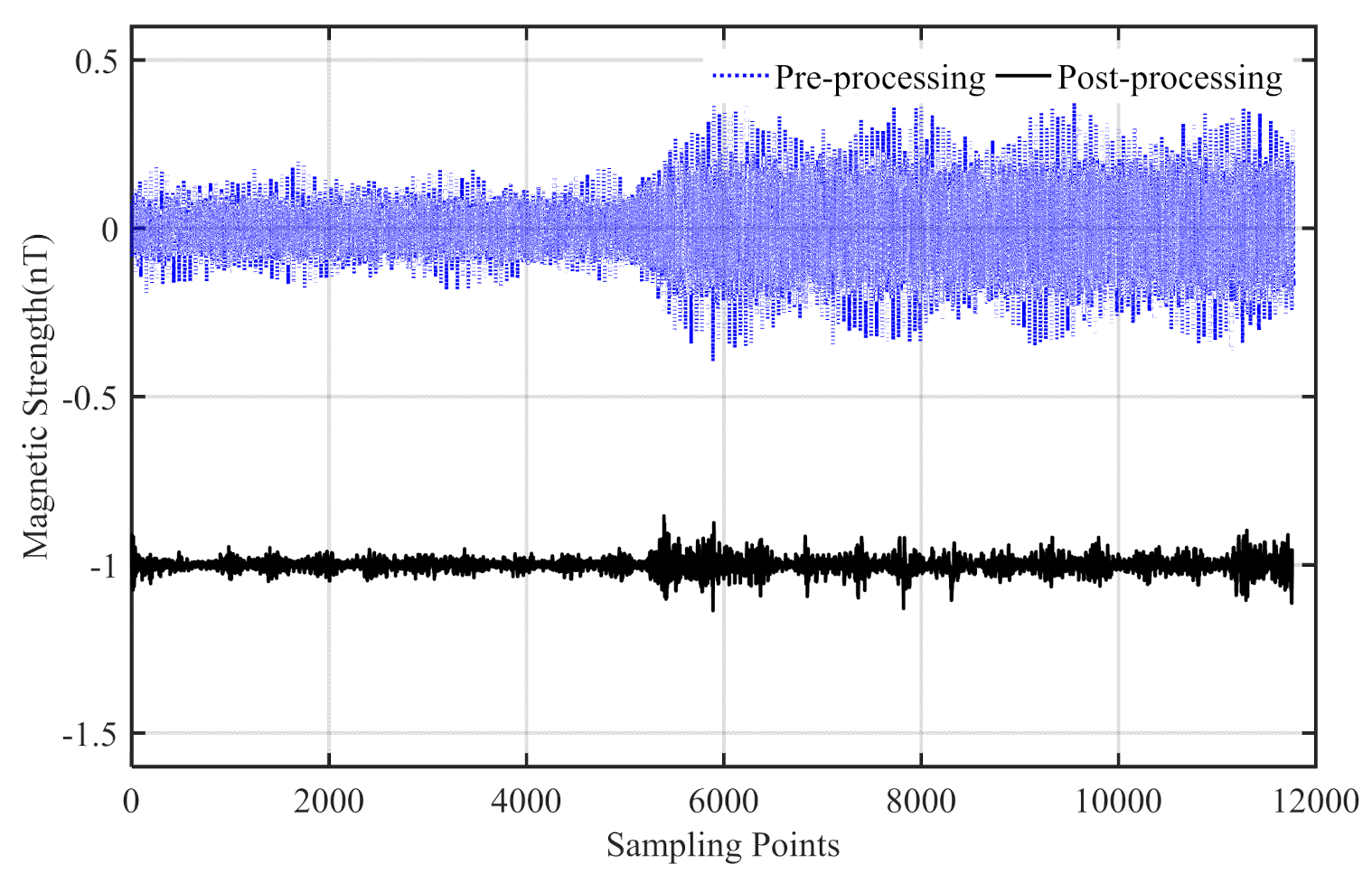
5.1.2. Results of the Improved Coherent Noise Suppression Method

For the same calibration flight data, the results using the ICNS method are shown in Figure 10 and Figure 11. The blue dot and black solid line represent the compensated field before and after the ICNS method, respectively. In Figure 11, the multi-frequency point interference fields were mostly eliminated by the proposed method. However, some of the interference fields were still not eliminated, which may have originated from the random motion of the carrier.

By comparing the results in Figure 9 and Figure 11, it can be seen that the ICNS method had a better suppression effect on the vibration interference magnetic field of the helicopter platform than the common AIC method if the two magnetometers were used. In order to further prove the effectiveness of the ICNS method proposed in this paper, Section 5.2 presents a simulation target design for the low-frequency magnetic field detection experiment to verify the effectiveness of this method.

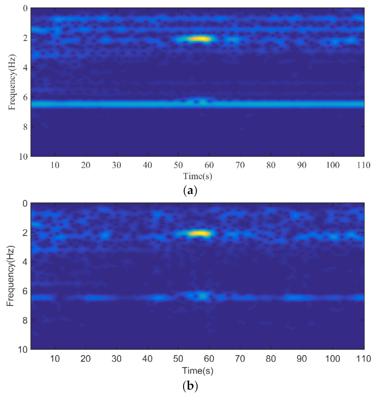
5.2. The Results of the Detection Experiment of Target

The magnetic signal was produced by a square closed coil, which was placed at the position of (30°23′45″ N, 111°56′45″ E). The excitation current was in a square wave with a peak value of 4A at 2.08 Hz. The coil position and flight lines are shown in Figure 12. The flight test consisted of two lines above the analog signal source. The flight altitude of the survey line was about 500 m, as shown in Figure 12b.

When the signal source was shut off, the measured magnetic field contained only the background field, and the measurement result of line 1 is shown in Figure 13. The interference field was eliminated by the proposed method. The blue dot line is the compensated data before the AIC method, the red dash line is the compensated data after the AIC method, and the black solid line is the compensated data after the ICNS method.

When the signal source was turned on, the measured magnetic field contained the background field and the low-frequency signal, and the measured result of line 1 is shown in Figure 14, where the blue dot line shows the compensated data before the AIC method, the red dash line shows the compensated data after the AIC method, and the black solid line is the compensated data after the ICNS method. It can be seen that the AIC method had little effect on the low-frequency signal. Meanwhile, the ICNS method eliminated most of the interference fields. In order to better show the processing results of the signal, the time–frequency diagram is given in Figure 15. It can be seen that the processed target signal was more obvious at 2.08 Hz and the harmonic frequency of 6.24 Hz than the original signal, as shown in Figure 15b.

5.3. The Discussion of the Results

Through the processing of the compensation and detection survey flight data, the effectiveness of the algorithm proposed in this paper was well confirmed. Through the analysis of the results of the experiment, the conclusions can be summarized as follows:

(1)

The traditional T–L aeromagnetic compensation model can only eliminate the interference magnetic field associated with the attitude of the manned helicopter, and its effective working frequency band is generally lower than 2 Hz.

(2)

The ICNS-based method proposed in this paper can eliminate the interference field caused by the probe vibration and has little influence on the target signal, so it can effectively improve the detection capability of the helicopter system for low-frequency target signals.

(3)

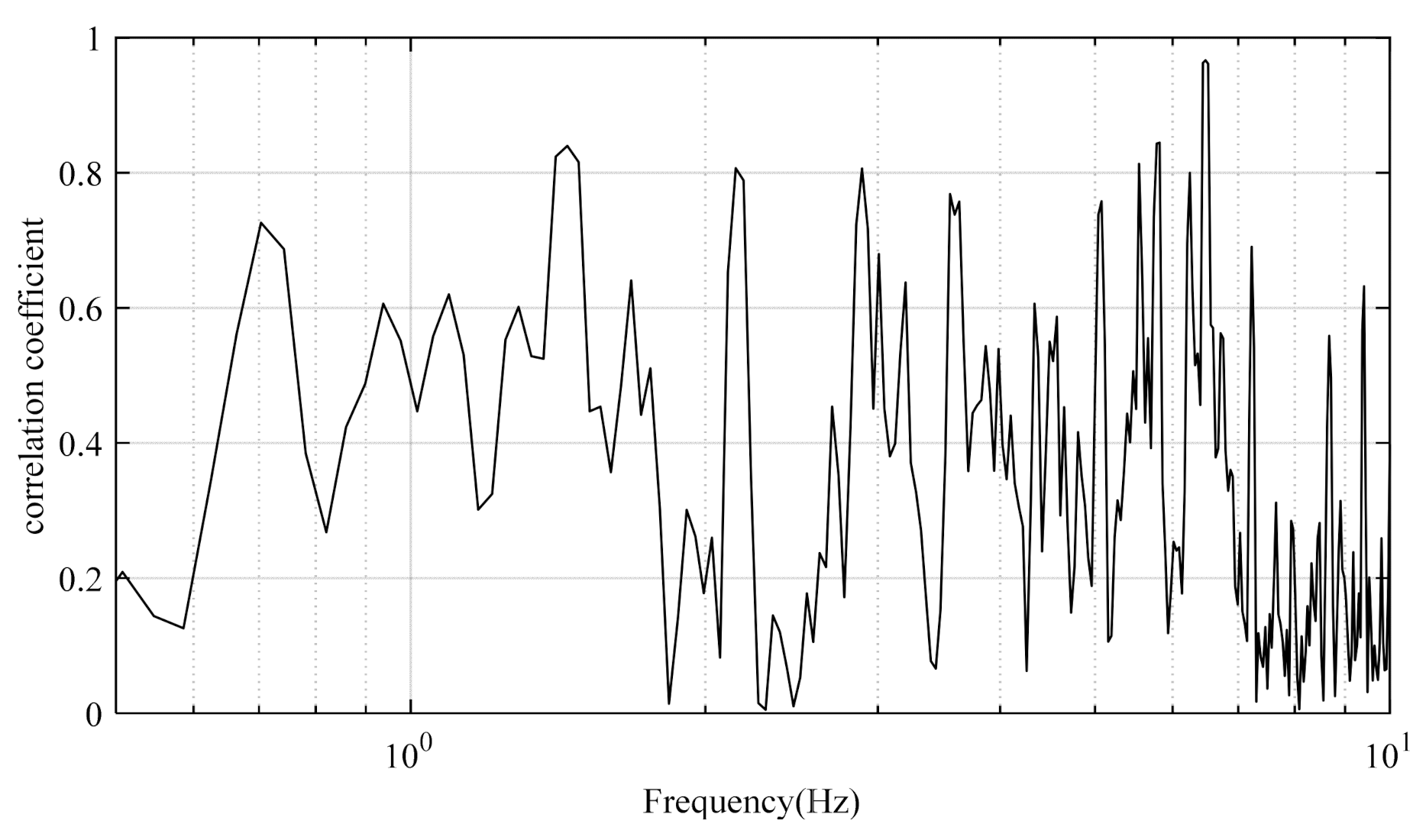
The ICNS-based method can be used for the vibration magnetic field interference during the movement of the aircraft if the interference field has obvious correlation characteristics with a pair of magnetometers.

6. Conclusions

The vibration magnetic interference that is caused by the mechanical motion of the probe has a significant influence on the detection performance of low-frequency magnetic field of a helicopter aeromagnetic system. The traditional aeromagnetic compensation (T–L) model considers only the interference magnetic fields that are related to the attitude of the aircraft and is generally suitable for compensation with a frequency below 2 Hz. To eliminate these interference magnetic fields, a method based on the improved coherent noise suppression method (ICNS) with a pair of magnetometers is proposed in this paper. Since the distance between the two magnetometers and the helicopter is far less than the distance between the helicopter and the target, the ICNS method can adaptively eliminate the vibration interference fields and has little effect on the field to be measured. The results of the calibration and detection with a flight test show that the proposed method can effectively eliminate the interference field that is caused by the vibration in accordance with the approaching target. The proposed algorithm shows its effectiveness in detecting ocean targets that generate low-frequency magnetic field signals or anomalies.

References

1. Ioannidis, G. Identification of a Ship or Submarine from its Magnetic Signature. IEEE Trans. Aerosp. Electron. Syst. 1977, AES-13, 327–329. [Google Scholar] [CrossRef]
2. Zolotarevskii, Y.M.; Bulygin, F.V.; Ponomarev, A.N.; Narchev, V.A.; Berezina, L.V. Methods of Measuring the Low-Frequency Electric and Magnetic Fields of Ships. Meas. Tech. 2005, 48, 1140–1144. [Google Scholar] [CrossRef]
3. Birsan, M. Measurement of the extremely low frequency (ELF) magnetic field emission from a ship. Meas. Sci. Technol. 2011, 22, 085709. [Google Scholar] [CrossRef]
4. Wu, Z.; Zhu, X.; Li, B. Modeling and measurements of alternating magnetic signatures of ships. Sens. Transducers. 2015, 186, 161–167. [Google Scholar]
5. Sun, Y.; Lin, C.; Jia, W.; Zhai, G. Analysis and measurement of ship shaft-rate magnetic field in air. Prog. Electromagn. Res. M 2016, 52, 119–127. [Google Scholar] [CrossRef] [Green Version]
6. Nabighian, M.N.; Grauch, V.J.S.; Hansen, R.O.; LaFehr, T.R.; Li, Y.; Peirce, J.W.; Phillips, J.; Ruder, M.E. The historical development of the magnetic method in exploration. Geophysics 2005, 70, 3361. [Google Scholar] [CrossRef]
7. Doll, W.E.; Gamey, T.J.; Bell, D.T.; Beard, L.P.; Sheehan, J.R.; Norton, J.; Holladay, J.S.; Lee, J.L.C. Historical Development and Performance of Airborne Magnetic and Electromagnetic Systems for Mapping and Detection of Unexploded Ordnance. J. Environ. Eng. Geophys. 2012, 17, 1–17. [Google Scholar] [CrossRef]
8. Hardwick, C.D. Non-oriented cesium sensors for airborne magnetometry and gradiometry. Explor. Geophys. 1984, 2, 266–267. [Google Scholar]
9. Tolles, W.E. Compensation of Aircraft Magnetic Fields. U.S. Patent 2692970A, 26 October 1954. [Google Scholar]
10. Tolles, W.E.; Mineola, N.Y. Magnetic Field Compensation System. U.S. Patent US2706801A, 19 April 1955. [Google Scholar]
11. Leliak, P. Identification and Evaluation of Magnetic-Field Sources of Magnetic Airborne Detector Equipped Aircraft. IRE Trans. Aeronaut. Navig. Electron. 1961, ANE-8, 95–105. [Google Scholar] [CrossRef]
12. Leach, B.W. Aeromagnetic compensation as a linear regression problem. In Information Linkage Between Applied Mathematics and Industry; Academic Press: New York, NY, USA, 1980; pp. 139–161. [Google Scholar]
13. Hardwick, C.D. Aeromagnetic Gradiometry in 1995. Explor. Geophys. 1996, 27, 1–11. [Google Scholar] [CrossRef]
14. Nelson, J.B. Aeromagnetic Noise during Low-Altitude Flights over the Scotian Shelf; DRDC-ATLANTIC, Defence R&D Canada: Ottawa, ON, Canada, 2002. [Google Scholar]
15. Nelson, J.B. Predicting In-Flight Mad Noise from Ground Measurements; DRDC-ATLANTIC, Defence R&D Canada: Ottawa, ON, Canada, 2001. [Google Scholar]
16. Noriega, G. Performance measures in aeromagnetic compensation. Lead. Edge 2011, 30, 1122–1127. [Google Scholar] [CrossRef]
17. Noriega, G. Model stability and robustness in aeromagnetic compensation. First Break 2013, 31, 73–79. [Google Scholar] [CrossRef]
18. Sheinker, A.; Moldwin, M.B. Adaptive interference cancelation using a pair of magnetometers. IEEE Trans. Aerosp. Electron. Syst. 2016, 52, 307–318. [Google Scholar] [CrossRef]
Figure 1. The helicopter platform and equipment.
Applsci 12 02065 g001
Figure 2. Calibration flight path in Google Earth (a) and its scale drawing (b).
Applsci 12 02065 g002
Figure 3. Compensation results of OPM-I: (a) calibration flight data and (b) the power spectral density of the calibration flight data.
Applsci 12 02065 g003
Figure 4. Compensation results of OPM-II: (a) calibration flight data and (b) the power spectral density of the calibration flight data.
Applsci 12 02065 g004
Figure 5. The correlation coefficient of the interference field in OPM-I and OPM-II.
Applsci 12 02065 g005
Figure 6. The model used for the adaptive interference cancelation method.
Applsci 12 02065 g006
Figure 7. Block diagram of the improved coherent noise suppression (ICNS) method.
Applsci 12 02065 g007
Figure 8. The pre-processing and post-processing results of the calibration flight data using AIC method.
Applsci 12 02065 g008
Figure 9. The time–frequency diagrams of the pre-processing (a) and post-processing (b) data using AIC method.
Applsci 12 02065 g009
Figure 10. The pre-processing and post-processing results of the calibration flight data using ICNS method.
Applsci 12 02065 g010
Figure 11. The time–frequency diagrams of the pre-processing (a) and post-processing (b) data using ICNS method.
Applsci 12 02065 g011
Figure 12. The flight path in Google Earth (a) and its scale drawing (b).
Applsci 12 02065 g012
Figure 13. The pre-processing and post-processing results of the survey line without the target.
Applsci 12 02065 g013
Figure 14. The pre-processing and post-processing results of the survey line with the target.
Applsci 12 02065 g014
Figure 15. The time–frequency diagrams of the survey line with the target, the pre-processing data (a), post-processing data with AIC method (b) and post-processing data with ICNS method (c).
Applsci 12 02065 g015aApplsci 12 02065 g015b