Almost Anti-Periodic Discrete Oscillation of General N-Dimensional Mechanical System and Underactuated Euler-Lagrange System

Abstract

In this paper, we introduce the notions of the almost anti-periodic discrete process of the N-dimensional vector-valued and $N\times N$ matrix-valued functions. Some basic properties of the almost anti-periodic discrete functions are established. Based on this, the conditions of the stability and instability of the almost anti-periodic solutions to the general N-dimensional mechanical system and the underactuated Euler–Lagrange system have been considered. Moreover, some examples are provided to support our obtained results.

1. Introduction

Almost periodic oscillation is a hot research field in the study of dynamic equations (see [1,2,3,4,5,6,7,8,9,10,11,12,13,14,15,16,17,18,19,20,21]). In recent years, many results of the various types of dynamic equations have been established related to almost periodic background including the results of the almost periodic analysis on the stochastic dynamic equations, fuzzy dynamic equations, and the dynamic equations on hybrid domains (see [3,12,13,14,16,17,18,19,20,22,23,24]). Based on the theory of translation closedness for time scales, the almost periodic functions and their generalizations were well defined and applied to study different types of dynamic models on time scales (see [1,3,12,13,14,15,16,17,18,19,20,23,25,26,27,28,29]).

On the other hand, another important phenomenon called anti-periodic oscillation was widely studied in the last ten years, and many results were established (see [5,6,10,11,30]). Anti-periodic functions were widely used in homogenization theory for composite materials and the continualization of discrete lattices (see [31,32]). It is well known that although anti-periodic oscillation belongs to a periodic oscillation, it is able to reflect a more particularly accurate oscillation in a period through the switch of its oscillation direction, and it has been widely applied in many interdisciplines (see [4,5,6,8,9,10,11,12,13,14,17,18,19,20,21,23,25,26,27,28,29,30,33,34]).

In 2017, M. Kostić introduced an interesting notion of almost anti-periodic functions in Banach space and studied the relationship between the types of anti-periodic functions and almost periodic functions in Banach spaces. After this, some related works were published (see [8,9,30,33,34]). It is natural to ask how to define the almost anti-periodic discrete process and explore what properties they will possess. The answer of this question will make it possible to study the almost anti-periodic discrete dynamic equation and contribute to establishing almost anti-periodic results on time scales.

Motivated by the above, the main aim of this work is to introduce the notion of the almost anti-periodic discrete process of the N-dimensional vector-valued and $N\times N$ matrix-valued functions and to establish the stability of the almost anti-periodic discrete solutions to the general N-dimensional mechanical system and underactuated Euler–Lagrange system. For some relating the finite-dimensional vector spaces, one may see [35] and the underactuated Euler–Lagrange system with N degrees of freedom and m independent controls (see [36]), as well as the general N-dimensional mechanical system (see [4]).

2. Almost Anti-Periodic Discrete Functions

In this section, we will introduce the notions of the almost anti-periodic discrete functions for the $N\times N$ matrix-valued function and the N-dimensional vector-valued function and establish some of their basic properties.

Definition 1.

Let $M(·)={\left[m_{ij}(·)\right]}_{N\times N}:\mathbb{Z}\to {\mathbb{R}}^{N\times N}$ be an $N\times N$ matrix-valued discrete function and $p(·)={[p_1(·),\dots ,p_N(·)]}^T:\mathbb{Z}\to {\mathbb{R}}^N$ be a N-dimensional vector-valued discrete function, we define

$$\parallel M\left(n\right)\parallel =\frac{1}{N^2}\sum _{j=1}^N\sum _{i=1}^N{\displaystyle |}{m}_{ij}\left(n\right)|,\parallel p\left(n\right)\parallel =\frac{1}{N}\sum _{j=1}^N\left|p_j\left(n\right)\right|.$$

If for $\forall \epsilon >0$, there exists a positive integer $l\left(\epsilon \right)$ and $\tau \in {[m,m+l]}_{\mathbb{Z}},\forall m\in \mathbb{Z}$, such that $p\left(n\right)$ satisfies the following condition

$$\parallel p(n+\tau )+p\left(n\right)\parallel <\epsilon ,\forall n\in \mathbb{Z}.$$

Then, $p\left(n\right)$ is called the almost anti-periodic discrete function, τ is called the ε-almost anti-period of $p\left(n\right)$, and l is called an inclusion length. Similarly, $M\left(n\right)$ is an almost anti-periodic $N\times N$ matrix-valued discrete function if

$$\parallel M(n+\tau )+M\left(n\right)\parallel <\epsilon ,\forall n\in \mathbb{Z}.$$

The set of all almost anti-periodic $N\times N$ matrix-valued discrete functions is denoted by $\mathfrak{G}$.

Definition 2

([30]). Let $\left\{q\right(n\left)\right\}$ be a discrete sequence, if for $\forall \epsilon >0$, there exists a positive integer $l\left(\epsilon \right)$ such that $q\left(n\right)$ satisfies the following condition

$$\left|q\right(n+\tau )-q(n\left)\right|<\epsilon ,\forall n\in \mathbb{Z}$$

for some $\tau \in {[m,m+l]}_{\mathbb{Z}}$, where $m\in \mathbb{Z}$. Then, $q\left(n\right)$ is called the almost periodic discrete function and τ is called the ε-almost period of $q\left(n\right)$.

Lemma 1.

Let $M\left(n\right)$ be an almost anti-periodic discrete function; then, it is an almost periodic discrete function.

Proof. 

By Definition 1, we have

$$\parallel M(n+2\tau )-M\left(n\right)\parallel \le \left|M\right(n+2\tau )+M(n+\tau )\parallel +\parallel M(n+\tau )+M(n)\parallel <2\epsilon .$$

The proof is completed. □

Through Lemma 1, the following lemma is immediate.

Lemma 2

([26]). Let $M\left(n\right)$ be an almost periodic discrete function (or an almost anti-periodic discrete function). Then, $\parallel M(·)\parallel :\mathbb{Z}\to \mathbb{R}$ is bounded.

In what follows, some basic properties of the almost anti-periodic discrete functions will be established.

Theorem 1.

Let $M(·)\in \mathfrak{G}$, then $cM(·)\in \mathfrak{G}$ for all $c\in \mathbb{R}$.

Proof. 

By Definition 1, one has

$$\parallel M(n+\tau )+M\left(n\right)\parallel <\frac{\epsilon }{\left|c\right|}$$

for $c\ne 0$. Thus, we have

$$\parallel cM(n+\tau )+cM\left(n\right)\parallel \le \left|c\right|\parallel M(n+\tau )+M\left(n\right)\parallel <\left|c\right|\frac{\epsilon }{\left|c\right|}=\epsilon ,$$

which means $cM(·)\in \mathfrak{G}$. For $c=0$, one can obtain the desired result. The proof is completed. □

Theorem 2.

Let $M(·)\in \mathfrak{G}$ and $Q\left(n\right)=M(n+k)$ for some $k\in \mathbb{Z}$. Then, $Q(·)\in \mathfrak{G}$.

Proof. 

Since $M(·)\in \mathfrak{G}$, we have

$$\parallel M(n+\tau )+M\left(n\right)\parallel <\epsilon \mathrm{for}\mathrm{all}n\in \mathbb{Z}.$$

Hence,

$$\parallel M(n+k+\tau )+M(n+k)\parallel <\epsilon ,n\in \mathbb{Z},$$

i.e.,

$$\parallel Q(n+\tau )+Q\left(n\right)\parallel <\epsilon ,n\in \mathbb{Z},$$

which implies $Q(·)\in \mathfrak{G}$. The proof is completed. □

Theorem 3.

Let $B(·)\in \mathfrak{G}$ and $S\left(n\right)$ be a summable $N\times N$ matrix sequence, i.e.,

$$S_0=\sum _{n\in \mathbb{Z}}\parallel S\left(n\right)\parallel <\infty .$$

If $M\left(n\right)={\displaystyle \sum _{m\in \mathbb{Z}}}S\left(m\right)B(n-m)$ for $n\in \mathbb{Z}$. Then, $M(·)\in \mathfrak{G}$.

Proof. 

Since $S\left(n\right)$ is a summable matrix sequence, for $\forall \epsilon >0$, there exists $N_0>0$ such that

$$\sum _{\left|n\right|>N_0}\parallel S\left(n\right)\parallel <\epsilon .$$

By Definition 1 and Theorem 2, one has

$$\parallel B(n+\tau -m)+B(n-m)\parallel <\frac{\epsilon }{S_0}.$$

By Lemma 2, we have $\parallel B\left(n\right)\parallel <\lambda$ for some $\lambda >0$ and any $n\in \mathbb{Z}$. Hence, we have

$$\begin{array}{cc}\hfill \parallel M(n+\tau )+M\left(n\right)\parallel & = \parallel {\displaystyle \sum _{m\in \mathbb{Z}}}S\left(m\right)B(n+\tau -m)+{\displaystyle \sum _{m\in \mathbb{Z}}}S\left(m\right)B(n-m)\parallel \hfill \\ \hfill & \le \parallel {\displaystyle \sum _{\left|m\right|\le N_0}}S\left(m\right)B(n+\tau -m)+{\displaystyle \sum _{\left|m\right|\le N_0}}S\left(m\right)B(n-m)\parallel \hfill \\ \hfill & +\parallel {\displaystyle \sum _{\left|m\right|>N_0}}S\left(m\right)B(n+\tau -m)+{\displaystyle \sum _{\left|m\right|>N_0}}S\left(m\right)B(n-m)\parallel \hfill \\ \hfill & \le \parallel {\displaystyle \sum _{\left|m\right|\le N_0}}S\left(m\right)\parallel \parallel B(n+\tau -m)+B(n-m)\parallel \hfill \\ \hfill & +\parallel {\displaystyle \sum _{\left|m\right|>N_0}}S\left(m\right)B(n+\tau -m)\parallel +\parallel {\displaystyle \sum _{\left|m\right|>N_0}}S\left(m\right)B(n-m)\parallel \hfill \\ \hfill & \le S_0\frac{\epsilon }{S_0}+\parallel {\displaystyle \sum _{\left|m\right|>N_0}}S\left(m\right)\parallel \lambda +\parallel {\displaystyle \sum _{\left|m\right|>N_0}}S\left(m\right)\parallel \lambda \le \epsilon +2\lambda ϵ,\hfill \end{array}$$

which means $M(·)\in \mathfrak{G}$. The proof is completed. □

Theorem 4.

Let $M(·)\in \mathfrak{G}$, then $\parallel M\left(n\right)\parallel$ is an almost periodic discrete function.

Proof. 

Since $M(·)\in \mathfrak{G}$, we have

$$\parallel M(n+\tau )+M\left(n\right)\parallel <\epsilon ,n\in \mathbb{Z}.$$

Hence,

$$\begin{array}{cc}\hfill |\parallel M(n+\tau )\parallel -\parallel M(n)\parallel |& =\left|\frac{1}{N^2}{\displaystyle \sum _{j=1}^N}{\displaystyle \sum _{i=1}^N}|m_{ij}(n+\tau )| - \frac{1}{N^2}{\displaystyle \sum _{j=1}^N}{\displaystyle \sum _{i=1}^N}\left|m_{ij}\left(n\right)\right|\right|\hfill \\ \hfill & \le \frac{1}{N^2}{\displaystyle \sum _{j=1}^N}{\displaystyle \sum _{i=1}^N}\left|\right|m_{ij}(n+\tau )| - |m_{ij}\left(n\right)\left|\right|\hfill \\ \hfill & \le \frac{1}{N^2}{\displaystyle \sum _{j=1}^N}{\displaystyle \sum _{i=1}^N}|m_{ij}(n+\tau )+m_{ij}\left(n\right)|\hfill \\ \hfill & = \parallel M(n+\tau )+M\left(n\right)\parallel <\epsilon ,\hfill \end{array}$$

which means that $\{\parallel M(n)\parallel \}$ is an almost periodic discrete function. The proof is completed. □

Based on the theorems above, the following result can be proved.

Proposition 1.

Let $M(·)\in \mathfrak{G}$, $c>0$, if $\parallel M\left(n\right)\parallel \ge c>0$. Then, the following limit exists:

$$\underset{n\to \infty }{lim}{\left[\prod _{j=1}^n\parallel M\left(j\right)\parallel \right]}^{\frac{1}{n}}.$$

(1)

Proof. 

Let $h\left(n\right)={\left[{\displaystyle \prod _{j=1}^n}\parallel M\left(j\right)\parallel \right]}^{\frac{1}{n}}$, we have

$$ln\left[h\right(n\left)\right]=\frac{1}{n}\left[\sum _{j=1}^{n}ln\parallel M\left(j\right)\parallel \right].$$

Step 1. We will prove that $\parallel M\left(n\right)\parallel$ is bounded. Since $M\left(n\right)$ is almost anti-periodic, by Theorem 4, we obtain $\parallel M\left(n\right)\parallel$, which is almost periodic. Moreover, by Lemma 2, one has $\parallel M\left(n\right)\parallel$, which is bounded; i.e., there exists $\lambda \in {\mathbb{R}}^{+}$ such that ${sup}_{n\in \mathbb{Z}}|ln\parallel M(n)\parallel |=\lambda$.

Step 2. We will prove that $ln\parallel M\left(n\right)\parallel$ is an almost periodic discrete function. Since $f\left(x\right)=lnx$ is uniformly continuous on $\left[c,e^{\lambda }\right]$, i.e., for $\forall \epsilon >0$, there exists $\delta \left(\epsilon \right)>0$ such that $|x_1-x_2|<\delta$ implies

$$|f\left(x_1\right)-f\left(x_2\right)|<\epsilon ,$$

for $x_1,x_2\in \left[c,e^{\lambda }\right]$. On the other hand, $M(·)\in \mathfrak{G}$, i.e.,

$$\parallel M(\tau +n)+M\left(n\right)\parallel <\epsilon .$$

By Theorem 4, one has

$$|\parallel M(\tau +n)\parallel -\parallel M(n)\parallel |<\epsilon .$$

By Step 1 and $\parallel M\left(n\right)\parallel \ge c>0$, we have $\parallel M\left(n\right)\parallel \in \left[c,e^{\lambda }\right]$. Thus, one has

$$|ln\parallel M(n+\tau )\parallel -ln\parallel M\left(n\right)\parallel |<\epsilon \mathrm{for}\mathrm{all}n\in \mathbb{Z},$$

which means that $ln\parallel M\left(n\right)\parallel$ is almost periodic, i.e., for $\forall \epsilon >0$, there exists a positive integer $l_0\left(\epsilon \right)$ such that $M\left(n\right)$ satisfies the following condition:

$$|ln\parallel M(n+\tau )\parallel -ln\parallel M\left(n\right)\parallel |<\epsilon ,n\in \mathbb{Z},$$

for some $\tau \in {[a,a+l_0]}_{\mathbb{Z}}$ and $a\in \mathbb{Z}$.

Step 3. By Step 2, for $\tau \in {[a,a+l_0]}_{\mathbb{Z}}$ and $\forall \frac{\epsilon }{4}>0$, there exists an positive integer $l_0\left(\epsilon \right)$ such that $M\left(n\right)$ satisfies the following condition:

$$|ln\parallel M(n+\tau )\parallel -ln\parallel M\left(n\right)\parallel |<\frac{\epsilon }{4},n\in \mathbb{Z},$$

for some $\tau \in {[a,a+l_0]}_{\mathbb{Z}}$ and $a\in \mathbb{Z}$. Next, we will consider $\tau =a$ and $\tau \in {(a,a+l_0]}_{\mathbb{Z}}$ cases.

Cases $\mathrm{I}$. $\tau =a$. Let $b\in {\mathbb{Z}}^{+}$, one has

$$\begin{array}{cc}\hfill |{\displaystyle \sum _{j=a+1}^{a+b}}ln\parallel M\left(j\right)\parallel -{\displaystyle \sum _{j=1}^b}ln\parallel M\left(j\right)\parallel |& =|{\displaystyle \sum _{j=\tau +1}^{\tau +b}}ln\parallel M\left(j\right)\parallel -{\displaystyle \sum _{j=1}^b}ln\parallel M\left(j\right)\parallel |\hfill \\ \hfill & \le {\displaystyle \sum _{j=1}^b}|ln\parallel M(j+\tau )\parallel -ln\parallel M\left(j\right)\parallel |\le \frac{\epsilon b}{4}.\hfill \end{array}$$

Cases $\mathrm{II}$. $\tau \in {(a,a+l_0]}_{\mathbb{Z}}$. By Step 2, for $b\in {\mathbb{N}}^{+}$, one has

$$\begin{array}{cc}\hfill & |{\displaystyle \sum _{j=a+1}^{a+b}}ln\parallel M\left(j\right)\parallel -{\displaystyle \sum _{j=1}^b}ln\parallel M\left(j\right)\parallel |\hfill \\ \hfill =& |{\displaystyle \sum _{j=\tau +1}^{\tau +b}}ln\parallel M\left(j\right)\parallel -{\displaystyle \sum _{j=1}^b}ln\parallel M\left(j\right)\parallel +{\displaystyle \sum _{j=a+1}^{\tau }}ln\parallel M\left(j\right)\parallel -{\displaystyle \sum _{j=a+b+1}^{\tau +b}}ln\parallel M\left(j\right)\parallel |\hfill \\ \hfill \le & {\displaystyle \sum _{j=1}^b}|ln\parallel M(j+\tau )\parallel -ln\parallel M\left(j\right)\parallel |+{\displaystyle \sum _{j=a+1}^{\tau }}|ln\parallel M\left(j\right)\parallel |+{\displaystyle \sum _{j=a+b+1}^{\tau +b}}|ln\parallel M\left(j\right)\parallel |\hfill \\ \hfill \le & \frac{\epsilon b}{4}+2l_0\lambda .\hfill \end{array}$$

Moreover, for the case $\mathrm{I}$, through taking $a=(k-1)n,$$b=n$, we have

$$|\sum _{j=(k-1)n+1}^{kn}ln\parallel M\left(j\right)\parallel -\sum _{j=1}^{n}ln\parallel M\left(j\right)\parallel |\le \frac{\epsilon n}{4};$$

for the case $\mathrm{II}$, through taking $a=(k-1)n,$$b=n$, one has

$$|\sum _{j=(k-1)n+1}^{kn}ln\parallel M\left(j\right)\parallel -\sum _{j=1}^{n}ln\parallel M\left(j\right)\parallel |\le \frac{\epsilon n}{4}+2l_0\lambda .$$

Step 4. We will prove that the Limit (1) exists. For any $m,n\in {\mathbb{N}}^{+}$, one has

$$\begin{array}{cc}\hfill |\frac{1}{n}{\displaystyle \sum _{j=1}^n}ln\parallel M\left(j\right)\parallel -\frac{1}{m}{\displaystyle \sum _{j=1}^m}ln\parallel M\left(j\right)\parallel |& \le \frac{1}{mn}|m{\displaystyle \sum _{j=1}^n}ln\parallel M\left(j\right)\parallel -{\displaystyle \sum _{j=1}^{mn}}ln\parallel M\left(j\right)\parallel |\hfill \\ \hfill & +\frac{1}{mn}|{\displaystyle \sum _{j=1}^{mn}}ln\parallel M\left(j\right)\parallel -n{\displaystyle \sum _{j=1}^m}ln\parallel M\left(j\right)\parallel |\hfill \\ \hfill & \le \frac{1}{mn}\left[{\displaystyle \sum _{k=1}^m}\right|{\displaystyle \sum _{j=(k-1)n+1}^{kn}}ln\parallel M\left(j\right)\parallel -{\displaystyle \sum _{j=1}^n}ln\parallel M\left(j\right)\parallel |\hfill \\ \hfill & +{\displaystyle \sum _{k=1}^n}|{\displaystyle \sum _{j=(k-1)m+1}^{km}}ln\parallel M\left(j\right)\parallel -{\displaystyle \sum _{j=1}^m}ln\parallel M\left(j\right)\parallel |].\hfill \end{array}$$

On the other hand, by Step 3, if $\tau =a=(k-1)n$, then

$$|\frac{1}{n}\sum _{j=1}^{n}ln\parallel M\left(j\right)\parallel -\frac{1}{m}\sum _{j=1}^{m}ln\parallel M\left(j\right)\parallel |\le \frac{1}{mn}(m\frac{\epsilon n}{4}+n\frac{\epsilon m}{4})=\frac{\epsilon }{2}<\epsilon ;$$

if $\tau \in {(a,a+l_0]}_{\mathbb{Z}}={((k-1)n,(k-1n)+l_0]}_{\mathbb{Z}}$, then

$$\begin{array}{cc}\hfill |\frac{1}{n}{\displaystyle \sum _{j=1}^n}ln\parallel M\left(j\right)\parallel -\frac{1}{m}{\displaystyle \sum _{j=1}^m}ln\parallel M\left(j\right)\parallel |& \le \frac{1}{mn}\left[m(\frac{\epsilon n}{4}+2l_0\lambda )+n\left(\frac{m\epsilon +2l_0}{4}\lambda \right)\right]\hfill \\ \hfill & =\frac{\epsilon }{2}+2l_0\lambda (\frac{1}{n}+\frac{1}{m})<\epsilon \hfill \end{array}$$

for $m,n\ge \left[\frac{8l_0\lambda }{\epsilon }\right]+1$, which indicates that the Limit (1) exists. The proof is completed. □

Proposition 2.

Let $M(·)\in \mathfrak{G}$. Then, the following limit equalities hold:

(i)

$h=\underset{n\to \infty }{lim}{\left[{\displaystyle \prod _{j=m+1}^{m+n}}\parallel M\left(j\right)\parallel \right]}^{\frac{1}{n}}=\underset{n\to \infty }{lim}{\left[{\displaystyle \prod _{j=1}^n}\parallel M\left(j\right)\parallel \right]}^{\frac{1}{n}}$.

(ii)

$h=\underset{n\to -\infty }{lim}{\left[{\displaystyle \prod _{j=n}^{-1}}\parallel M\left(j\right)\parallel \right]}^{-\frac{1}{n}}=\underset{n\to \infty }{lim}{\left[{\displaystyle \prod _{j=-n}^{-1}}\parallel M\left(j\right)\parallel \right]}^{\frac{1}{n}}$.

Proof. 

(i) Through using the process of the proof of Proposition 1, we can turn (i) into the following equality:

$$\underset{n\to \infty }{lim}\frac{1}{n}\left[\sum _{j=m+1}^{m+n}ln\parallel M\left(j\right)\parallel -\sum _{j=1}^{n}ln\parallel M\left(j\right)\parallel \right]=0.$$

(2)

By the proof of Proposition 1 Step 2, for $\forall \frac{\epsilon }{2}>0$, there exists a positive integer $l_0\left(\epsilon \right)$ such that $M\left(j\right)$ satisfies the following condition:

$$|ln\parallel M(j+\tau )\parallel -ln\parallel M\left(j\right)\parallel |\le \frac{\epsilon }{2}\mathrm{for}\mathrm{all}j\in \mathbb{Z},$$

where $\tau \in {[m,m+l]}_{\mathbb{Z}}$ and $m\in \mathbb{Z}$. Next, we will consider $\tau =m$ and $\tau \in {(m,m+l]}_{\mathbb{Z}}$ cases. By the proof of Proposition 1 Step 3, taking $a=m$ and $b=n$, the desired results can be shown.

Cases $\mathrm{I}$. $\tau =m$. For $\tau =m$, we have

$$\begin{array}{cc}\hfill & \frac{1}{n}|{\displaystyle \sum _{j=m+1}^{m+n}}ln\parallel M\left(j\right)\parallel -{\displaystyle \sum _{j=1}^n}ln\parallel M\left(j\right)\parallel |\hfill \\ \hfill =& \frac{1}{n}|{\displaystyle \sum _{j=\tau +1}^{\tau +n}}ln\parallel M\left(j\right)\parallel -{\displaystyle \sum _{j=1}^n}ln\parallel M\left(j\right)\parallel |\hfill \\ \hfill \le & \frac{1}{n}{\displaystyle \sum _{j=1}^n}|ln\parallel M(j+\tau )\parallel -ln\parallel M\left(j\right)\parallel |\le \frac{1}{n}\frac{\epsilon n}{2}<\epsilon .\hfill \end{array}$$

Therefore, Equation (2) holds.

Cases $\mathrm{II}$. $\tau \in {(m,m+l]}_{\mathbb{Z}}$. For $\tau \in {(m,m+l]}_{\mathbb{Z}}$, we have

$$\begin{array}{cc}\hfill & \frac{1}{n}|{\displaystyle \sum _{j=m+1}^{m+n}}ln\parallel M\left(j\right)\parallel -{\displaystyle \sum _{j=1}^n}ln\parallel M\left(j\right)\parallel |\hfill \\ \hfill =& \frac{1}{n}|{\displaystyle \sum _{j=\tau +1}^{\tau +n}}ln\parallel M\left(j\right)\parallel -{\displaystyle \sum _{j=1}^n}ln\parallel M\left(j\right)\parallel +{\displaystyle \sum _{j=m+1}^{\tau }}ln\parallel M\left(j\right)\parallel -{\displaystyle \sum _{j=m+n+1}^{\tau +n}}ln\parallel M\left(j\right)\parallel |\hfill \\ \hfill \le & \frac{1}{n}\left[{\displaystyle \sum _{j=1}^n}|ln\parallel M(j+\tau )\parallel -ln\parallel M\left(j\right)\parallel |+{\displaystyle \sum _{j=m+1}^{\tau }}|ln\parallel M\left(j\right)\parallel |+{\displaystyle \sum _{j=m+n+1}^{\tau +n}}|ln\parallel M\left(j\right)\parallel |\right]\hfill \\ \hfill \le & \frac{1}{n}(\frac{\epsilon n}{2}+2l\lambda )\le \epsilon \hfill \end{array}$$

for $n\ge \left[\frac{4l\lambda }{\epsilon }\right]+1.$ Hence, Equation (2) holds.

(ii) Through using the proof process of Proposition 1, we can turn (ii) into the following equality:

$$\underset{n\to -\infty }{lim}\frac{1}{-n}\sum _{j=-1}^{n}ln\parallel M\left(j\right)\parallel =\underset{n\to \infty }{lim}\frac{1}{n}\sum _{j=-1}^{-n}ln\parallel M\left(j\right)\parallel .$$

On the other hand, by the proof of Proposition 1 Step 2, we obtain that $ln\parallel M\left(n\right)\parallel$ is almost periodic discrete function. Hence,

$$\underset{n\to \infty }{lim}\frac{1}{n}\sum _{j=-1}^{-n}ln\parallel M\left(j\right)\parallel =\underset{n\to \infty }{lim}\frac{1}{n}\sum _{j=1}^{n}ln\parallel M\left(j\right)\parallel ,$$

i.e.,

$$\underset{n\to \infty }{lim}\frac{1}{n}\left[\sum _{j=-n}^{-1}ln\parallel M\left(j\right)\parallel -\sum _{j=1}^{n}ln\parallel M\left(j\right)\parallel \right]=0.$$

(3)

Similarly, by the proof of Proposition 1 Step 2, we have

$$|ln\parallel M(j+\tau )\parallel -ln\parallel M\left(j\right)\parallel |\le \frac{\epsilon }{2}\mathrm{for}\mathrm{all}j\in \mathbb{Z},$$

where $\tau \in {[-n-1,-n-1+l]}_{\mathbb{Z}}$. Next, we will consider the case for $\tau =-n-1$ and $\tau \in {(-n-1,-n-1+l]}_{\mathbb{Z}}$. By the proof of Proposition 1 Step 3, taking $a=-n-1$ and $b=n$, the desired results can be proved.

Cases $\mathrm{I}$. $\tau =-n-1$. For $\tau =-n-1$, we have

$$\begin{array}{cc}\hfill \frac{1}{n}|{\displaystyle \sum _{j=-n}^{-1}}ln\parallel M\left(j\right)\parallel -{\displaystyle \sum _{j=1}^n}ln\parallel M\left(j\right)\parallel |& =\frac{1}{n}|{\displaystyle \sum _{j=\tau +1}^{\tau +n}}ln\parallel M\left(j\right)\parallel -{\displaystyle \sum _{j=1}^n}ln\parallel M\left(j\right)\parallel |\hfill \\ \hfill & \le \frac{1}{n}\left[{\displaystyle \sum _{j=1}^n}|ln\parallel M(j+\tau )\parallel -ln\parallel M\left(j\right)\parallel |\right]\hfill \\ \hfill & \le \frac{1}{n}\frac{\epsilon }{2}n=\frac{\epsilon }{2}<\epsilon .\hfill \end{array}$$

Therefore, Equation (3) holds.

Cases $\mathrm{II}$. $\tau \in {(-n-1,-n-1+l]}_{\mathbb{Z}}$. For $\tau \in {(-n-1,-n-1+l]}_{\mathbb{Z}}$, it follows that

$$\begin{array}{cc}\hfill & \frac{1}{n}|{\displaystyle \sum _{j=-n}^{-1}}ln\parallel M\left(j\right)|-{\displaystyle \sum _{j=1}^n}ln\parallel M\left(j\right)\parallel |\hfill \\ \hfill =& \frac{1}{n}|{\displaystyle \sum _{j=\tau +1}^{\tau +n}}ln\parallel M\left(j\right)\parallel -{\displaystyle \sum _{j=1}^n}ln\parallel M\left(j\right)\parallel +{\displaystyle \sum _{j=-n}^{\tau }}ln\parallel M\left(j\right)\parallel -{\displaystyle \sum _{j=0}^{\tau +n}}ln\parallel M\left(j\right)\parallel |\hfill \\ \hfill \le & \frac{1}{n}\left[{\displaystyle \sum _{j=1}^n}|ln\parallel M(j+\tau )\parallel -ln\parallel M\left(j\right)\parallel |+{\displaystyle \sum _{j=-n}^{\tau }}|ln\parallel M\left(j\right)\parallel |+{\displaystyle \sum _{j=0}^{\tau +n}}|ln\parallel M\left(j\right)\parallel |\right]\hfill \\ \hfill \le & \frac{1}{n}\left(\frac{\epsilon n}{2}+2l\lambda \right)\le \epsilon \hfill \end{array}$$

for $n\ge \left[\frac{4l\lambda }{\epsilon }\right]+1.$ Hence, Equation (3) holds. The proof is completed. □

3. Almost Anti-Periodic Oscillation of the Mechanical System

In this section, we will consider the almost anti-periodic oscillation of the general mechanical systems.

3.1. Existence and Uniqueness of the Almost Anti-Periodic Solution

Consider the general N-dimensional mechanical system as follows:

$$B[(q(n+2)-2q(n+1)+q\left(n\right)]+C[q(n+1)-q\left(n\right)]+S\left(q\left(n\right)\right)=f\left(n\right),$$

(4)

where $q(·)=[q_1(·),\dots ,q_N(·)]\in {\mathbb{R}}^N$, $B,C\in {\mathbb{R}}^{N\times N}$ is symmetric and B is positive definite, the vector $S\left(q\right)$ collects all position dependent forces, such a linear and nonlinear stiffness forces or non-potential forces, $f\left(n\right)$ is an almost anti-periodic discrete function. Moreover, Equation (4) can be rewritten as

$$Bq(n+2)+(C-2B)q(n+1)+(B-C)q\left(n\right)+S\left(q\left(n\right)\right) =f\left(n\right).$$

Assume that $x\left(n\right)={[q\left(n\right),q(n+1)]}^T$, i.e.,

$$x\left(n\right)={[q_1\left(n\right),\dots ,q_N\left(n\right),q_1(n+1),\dots ,q_N(n+1)]}^T,$$

Equation (4) can be rewritten as

$$\begin{array}{cc}\hfill x(n+1)& = \left[\begin{array}{c}q(n+1)\\ q(n+2)\end{array}\right] = \left[\begin{array}{c}q(n+1)\\ \xi \end{array}\right] + \left[\begin{array}{c}0\\ f\left(n\right)-S\left(q\left(n\right)\right)\end{array}\right]\hfill \\ \hfill & = \left[\begin{array}{cc}0& I\\ B^{-1}(C-B)& B^{-1}(2B-C)\end{array}\right]\left[\begin{array}{c}q\left(n\right)\\ q(n+1)\end{array}\right]\hfill \\ \hfill & + \left[\begin{array}{c}0\\ B^{-1}f\left(n\right)-B^{-1}S\left(q\left(n\right)\right)\end{array}\right]\hfill \\ \hfill & =Rx\left(n\right)+b\left(n\right),\hfill \end{array}$$

(5)

where $\xi =B^{-1}(C-B)q\left(n\right)+B^{-1}(2B-C)q(n+1)$ and

$$R=\left[\begin{array}{cc}0& I\\ B^{-1}(C-B)& B^{-1}(2B-C)\end{array}\right],b\left(n\right)=\left[\begin{array}{c}0\\ B^{-1}f\left(n\right)-B^{-1}S\left(q\left(n\right)\right)\end{array}\right].$$

In the sequel, we will establish some sufficient conditions of the existence and uniqueness of the almost anti-periodic solution of Equation (5).

Theorem 5.

Let $s<n$, the unique solution of Equation (5) with the initial value condition $x\left(s\right)=x_0$ can be given as:

$$x\left(n\right)={[q\left(n\right),q(n+1)]}^T=R^{n-s}x\left(s\right)+\sum _{j=n-1-s}^0{R}^{j}b(n-1-j),$$

i.e.,

$$\begin{array}{c}x\left(n\right)={[q\left(n\right),q(n+1)]}^T={\left[\begin{array}{cc}0& I\\ B^{-1}(C-B)& B^{-1}(2B-C)\end{array}\right]}^{n-s}x\left(s\right)\\ +{\displaystyle \sum _{j=n-1-s}^0}{\left[\begin{array}{cc}0& I\\ B^{-1}(C-B)& B^{-1}(2B-C)\end{array}\right]}^j\left[\begin{array}{c}0\\ \eta \end{array}\right],\end{array}$$

where $R^0=I$, $\eta =B^{-1}f(n-1-j)-B^{-1}S\left(q(n-1-j)\right)$.

Proof. 

Step 1, we will prove the existence of the solution of Equation (4). For $n>s$, we have

$$\begin{array}{cc}\hfill x(n+1)& =R^{n+1-s}x\left(s\right)+{\displaystyle \sum _{j=n-s}^0}{R}^{j}b(n-j)\hfill \\ \hfill & =R^{n+1-s}x\left(s\right)+{\displaystyle \sum _{j=n-s}^1}{R}^{j}b(n-j)+b\left(n\right)\hfill \\ \hfill & =R\left[R^{n-s}x\left(s\right)+{\displaystyle \sum _{j=n-s}^1}{R}^{j-1}b(n-j)\right]+b\left(n\right)=Rx\left(n\right)+b\left(n\right)\hfill \end{array}$$

and $x\left(s\right)=x_0$, which means that $x\left(n\right)$ is a solution of Equation (4).

Step 2, we will prove the uniqueness of the solution of Equation (5). Let $x\left(n\right)$ and $y\left(n\right)$ be two solutions of Equation (5) with the initial value condition $x\left(s\right)=y\left(s\right)=x_0$, then we have

$$x\left(n\right)=Rx(n-1)+b(n-1)\mathrm{and}y\left(n\right)=Ry(n-1)+b(n-1).$$

Assume that $V\left(n\right)=x\left(n\right)-y\left(n\right)$, then $V\left(n\right)=RV(n-1)$. Hence,

$$V\left(n\right)=R^{n-s}V\left(s\right).$$

On the other hand, $x\left(s\right)=y\left(s\right)=x_0$, i.e., $V\left(s\right)=0$, which implies $V\left(n\right)=0$, i.e., $x\left(n\right)=y\left(n\right)$. The proof is completed. □

Lemma 3.

Let τ be a ε-almost anti-period of $f\left(n\right)$, if $\parallel R\parallel + \lambda \parallel B^{-1}\parallel <1-\lambda$, $\parallel R\parallel \le \lambda$, $\parallel S\left(q\right)+S\left(p\right)\parallel \le \frac{\lambda }{\parallel B^{-1}\parallel }\parallel p+q\parallel$ for $p,q\in {\mathbb{R}}^N$ and $0<\lambda <1$. Then,

$$\begin{array}{c}\parallel b(n+\tau )+b\left(n\right)\parallel \le \upsilon \parallel q(n+\tau )+q\left(n\right)\parallel \\ \parallel q(n+1+\tau )+q(n+1)\parallel <\zeta \parallel q(n+\tau )+q\left(n\right)\parallel \end{array}$$

where $\upsilon \in (\lambda ,1)$ and $0<\zeta =\frac{\parallel R\parallel +\lambda \parallel B^{-1}\parallel }{1-\parallel R\parallel }<1$.

Proof. 

Since $b\left(n\right)={\left[0,B^{-1}f\left(n\right)-B^{-1}S\left(q\left(n\right)\right)\right]}^T$, we have

$$\begin{array}{cc}\hfill \parallel b(n+\tau )+b\left(n\right)\parallel & = \parallel B^{-1}f(n+\tau )-B^{-1}S\left(q(n+\tau )\right) + B^{-1}f\left(n\right)-B^{-1}S\left(q\left(n\right)\right)\parallel \hfill \\ \hfill & \le \parallel B^{-1}f(n+\tau )+B^{-1}f\left(n\right)\parallel +\parallel B^{-1}S\left(q(n+\tau )\right) + B^{-1}S\left(q\left(n\right)\right)\parallel \hfill \\ \hfill & \le \parallel B^{-1}\parallel \epsilon + \parallel B^{-1}\parallel \frac{\lambda }{\parallel B^{-1}\parallel }\parallel q(n+\tau )+q\left(n\right)\parallel \hfill \\ \hfill & = \parallel B^{-1}\parallel \epsilon +\lambda \parallel q(n+\tau )+q\left(n\right)\parallel .\hfill \end{array}$$

Hence, there exists $\upsilon \in (\lambda ,1)$ such that $\parallel b(n+\tau )+b\left(n\right)\parallel \le \upsilon \parallel q(n+\tau )+q\left(n\right)\parallel$. On the other hand, $\tau$ is a $\epsilon$-almost anti-period of $f\left(n\right)$ and $x\left(n\right)={[p\left(n\right),p(n+1)]}^T$, we have

$$\begin{array}{cc}\hfill & \parallel x(n+1+\tau )+x(n+1)\parallel = \parallel q(n+1+\tau )+q(n+1)\parallel +\parallel q(n+2+\tau )+q(n+2)\parallel \hfill \\ \hfill =& \parallel Rx(n+\tau )+b(n+\tau )+Rx\left(n\right)+b\left(n\right)\parallel \hfill \\ \hfill \le & \parallel R\parallel \parallel x(n+\tau )+x\left(n\right)\parallel +\parallel b(n+\tau )+b\left(n\right)\parallel \hfill \\ \hfill \le & \parallel R\parallel \left(\parallel q(n+\tau )+q\left(n\right)\parallel +\parallel q(n+1+\tau )+q(n+1)\parallel \right)\hfill \\ \hfill +& \parallel B^{-1}\parallel \left(\parallel f(n+\tau )+f\left(n\right)\parallel +\parallel S\left(q\right(n+\tau \left)\right)+S\left(q\right(n\left)\right)\parallel \right)\hfill \\ \hfill \le & (\parallel R\parallel +\lambda \parallel B^{-1}\parallel )\parallel q(n+\tau )+q\left(n\right)\parallel +\parallel R\parallel \parallel q(n+1+\tau )+q(n+1)\parallel +\parallel B^{-1}\parallel \epsilon ,\hfill \end{array}$$

i.e.,

$$\begin{array}{c}\hfill (1-\parallel R\parallel )\parallel q(n+1+\tau )+q(n+1)\parallel +\parallel q(n+2+\tau )+q(n+2)\parallel \\ \hfill \le (\parallel R\parallel +\lambda \parallel B^{-1}\parallel )\parallel q(n+\tau )+q\left(n\right)\parallel + \parallel B^{-1}\parallel \epsilon .\end{array}$$

Hence,

$$\parallel q(n+1+\tau )+q(n+1)\parallel <\frac{\parallel R\parallel +\lambda \parallel B^{-1}\parallel }{1-\parallel R\parallel }\parallel q(n+\tau )+q\left(n\right)\parallel .$$

The proof is completed. □

Now, consider the underactuated Euler–Lagrange system with N degrees of freedom and m independent controls by a discrete dynamic equation as follows:

$$\begin{array}{ccc}\hfill & & B\left(q\left(n\right)\right)\left(q(n+2)-2q(n+1)+q\left(n\right)\right)\hfill \\ & & +C\left(q\left(n\right),q(n+1)-q\left(n\right)\right)[q(n+1)-q\left(n\right)]+G\left(q\left(n\right)\right)=L\omega ,\hfill \end{array}$$

(6)

where B is a positive definite matrix denoting the inertia matrix, C is the Coriolis matrix, G is the gravity vector, $L=[0,I_m]$, $q(·)=[q_1(·),\dots ,q_N(·)]\in {\mathbb{R}}^N$ is the generalised coordinate vector, and $\omega \in {\mathbb{R}}^m$ is the control. Assume that $x\left(n\right)={[q\left(n\right),q(n+1)]}^T$, Equation (6) can be rewritten as

$$\begin{array}{cc}\hfill & x(n+1)= \left[\begin{array}{c}q(n+1)\\ q(n+2)\end{array}\right]\hfill \\ \hfill =& \left[\begin{array}{c}q(n+1)\\ {\gamma }_{0}q\left(n\right)+{\gamma }_{1}q(n+1)\end{array}\right] + \left[\begin{array}{c}0\\ B^{-1}\left(q\left(n\right)\right)\left[L\omega -G\left(q\left(n\right)\right)\right]\end{array}\right]\hfill \\ \hfill =& \left[\begin{array}{cc}0& I\\ {\gamma }_0& {\gamma }_1\end{array}\right]x\left(n\right)+a\left(n\right)\hfill \\ \hfill =& H\left(n\right)x\left(n\right)+a\left(n\right),\hfill \end{array}$$

(7)

where

$${\gamma }_0=B^{-1}\left(q\left(n\right)\right)C(q\left(n\right),q(n+1)-q\left(n\right))-I,$$

$${\gamma }_1=2I-B^{-1}\left(q\left(n\right)\right)C(q\left(n\right),q(n+1)-q\left(n\right)),$$

and

$$\begin{array}{cc}\hfill H\left(n\right)=& \left[\begin{array}{cc}0& I\\ {\gamma }_0& {\gamma }_1\end{array}\right],a\left(n\right)= \left[\begin{array}{c}0\\ B^{-1}\left(q\left(n\right)\right)\left[L\omega -G\left(q\left(n\right)\right)\right]\end{array}\right].\hfill \end{array}$$

Theorem 6.

Let $s<n$, the unique solution (7) with the initial value $x\left(s\right)=x_0$ can be given as

$$x\left(n\right)=\left(\prod _{j=s}^{n-1}H\left(j\right)\right)x_0+\sum _{j=s}^{n-2}\left[\prod _{i=1}^{n-(j+1)}H(n-i)\right]a\left(j\right)+a(n-1).$$

Proof. 

The proof process is similar to the proof process of Theorem 5, we will not repeat it here. □

Lemma 4.

Let $\tau \in {\mathbb{Z}}^{+}$,

$$\begin{array}{c}\hfill \parallel B^{-1}\left(q\right)C(q,p)-I\parallel +\parallel 2I-B^{-1}\left(q\right)C(q,p)\parallel <\frac{\eta -\lambda }{1+\eta }-\frac{1}{N}<1-\frac{1}{N},\\ \hfill \parallel B^{-1}\left(q\right)[L\omega -G\left(q\right)] + B^{-1}\left(p\right)[L\omega -G\left(p\right)]\parallel \le \lambda \parallel p+q\parallel ,\\ \hfill \parallel H\left(n\right)a\left(n\right)+H\left(s\right)a\left(s\right)\parallel \le max\{\parallel H(n)\parallel ,\parallel H(s)\parallel \}\parallel a\left(n\right)+a\left(s\right)\parallel \end{array}$$

for any $p,q\in {\mathbb{R}}^N$, $n,s\in \mathbb{Z}$ and $0<\lambda <\eta <1$. Then,

$$\begin{array}{c}\hfill \parallel a(n+\tau )+a\left(n\right)\parallel \le \lambda \parallel q(n+\tau )+q\left(n\right)\parallel ,\\ \hfill \parallel q(n+1+\tau )+q(n+1)\parallel <\eta \parallel q(n+\tau )+q\left(n\right)\parallel ,\\ \hfill \parallel H(n+\tau )a(n+\tau )+H\left(n\right)a\left(n\right)\parallel \le max\{\parallel H(n+\tau )\parallel ,\parallel H(n)\parallel \}\parallel a(n+\tau )+a\left(n\right)\parallel .\end{array}$$

Proof. 

Since

$$a\left(n\right)= \left[\begin{array}{c}0\\ B^{-1}\left(q\left(n\right)\right)\left[L\omega -G\left(q\left(n\right)\right)\right]\end{array}\right],$$

we have

$$\begin{array}{cc}\hfill \parallel a(n+\tau )+a\left(n\right)\parallel =& \parallel B^{-1}\left(q(n+\tau )\right)\left[L\omega -G\left(q(n+\tau )\right)\right]\hfill \\ \hfill & +B^{-1}\left(q\left(n\right)\right)\left[L\omega -G\left(q\left(n\right)\right)\right]\parallel \hfill \\ \hfill \le & \lambda \parallel q(n+\tau )+q\left(n\right)\parallel \hfill \end{array}$$

and

$$\begin{array}{cc}\hfill & \parallel x(n+1+\tau )+x(n+1)\parallel \hfill \\ \hfill =& \parallel q(n+1+\tau )+q(n+1)\parallel +\parallel q(n+2+\tau )+q(n+2)\parallel \hfill \\ \hfill =& \parallel H\left(n\right)x(n+\tau )+a(n+\tau )+H\left(n\right)x\left(n\right)+a\left(n\right)\parallel \hfill \\ \hfill \le & \parallel H\left(n\right)\parallel \parallel x(n+\tau )+x\left(n\right)\parallel +\parallel a(n+\tau )+a\left(n\right)\parallel \hfill \\ \hfill \le & \parallel H\left(n\right)\parallel \left(\parallel q(n+\tau )+q\left(n\right)\parallel +\parallel q(n+1+\tau )+q(n+1)\parallel \right)+\lambda \parallel q(n+\tau )+q\left(n\right)\parallel ),\hfill \end{array}$$

i.e.,

$$\begin{array}{cc}\hfill & (1-\parallel H(n)\parallel )\parallel q(n+1+\tau )+q(n+1)\parallel +\parallel q(n+2+\tau )+q(n+2)\parallel \hfill \\ \hfill \le & (\parallel H(n)\parallel +\lambda )\parallel q(n+\tau )+q\left(n\right)\parallel .\hfill \end{array}$$

Hence,

$$\parallel q(n+1+\tau )+q(n+1)\parallel <\frac{\parallel H\left(n\right)\parallel +\lambda }{1-\parallel H\left(n\right)\parallel }\parallel q(n+\tau )+q\left(n\right)\parallel$$

and

$$\parallel q(n+2+\tau )+q(n+2)\parallel <(\parallel H\left(n\right)\parallel +\lambda \parallel B^{-1}\parallel )\parallel q(n+\tau )+q\left(n\right)\parallel .$$

On the other hand, since

$$H\left(n\right)= \left[\begin{array}{cc}0& I\\ {\gamma }_0& {\gamma }_1\end{array}\right],$$

where

$${\gamma }_0=B^{-1}\left(q\left(n\right)\right)C(q\left(n\right),q(n+1)-q\left(n\right))-I,$$

$${\gamma }_1=2I-B^{-1}\left(q\left(n\right)\right)C(q\left(n\right),q(n+1)-q\left(n\right)),$$

we have

$$\begin{array}{cc}\hfill \parallel H\left(n\right)\parallel =& \frac{1}{N^2}[N +\parallel B^{-1}\left(q\left(n\right)\right)C(q\left(n\right),q(n+1)-q\left(n\right))-I\parallel \hfill \\ \hfill +& \parallel 2I-B^{-1}\left(q\left(n\right)\right)C(q\left(n\right),q(n+1)-q\left(n\right))\parallel ]\hfill \\ \hfill \le & \frac{1}{N}+\frac{\eta -\lambda }{1+\eta }-\frac{1}{N}=\frac{\eta -\lambda }{1+\eta }<1,\hfill \end{array}$$

i.e., $\frac{\parallel H\left(n\right)\parallel +\lambda }{1-\parallel H\left(n\right)\parallel }<\eta$. Thus, $\parallel q(n+1+\tau )+q(n+1)\parallel <\eta \parallel q(n+\tau )+q\left(n\right)\parallel$. Since

$$\parallel H\left(n\right)a\left(n\right)+H\left(s\right)a\left(s\right)\parallel \le max\{\parallel H(n)\parallel ,\parallel H(s)\parallel \}\parallel a\left(n\right)+a\left(s\right)\parallel ,$$

we have

$$\parallel H(n+\tau )a(n+\tau )+H\left(n\right)a\left(n\right)\parallel \le max\{\parallel H(n+\tau )\parallel ,\parallel H(n)\parallel \}\parallel a(n+\tau )+a\left(n\right)\parallel .$$

The proof is completed. □

3.2. Stability of the Almost Anti-Periodic Solutions

In this section, we will establish the stability of the general N-dimensional mechanical system and the underactuated Euler–Lagrange system under the almost anti-periodic discrete process. Through Equations (5) and (7), the systems (4) and (6) can be turned into the following nonhomogeneous linear system

$$x(n+1)=M\left(n\right)x\left(n\right)+c\left(n\right),n\in \mathbb{Z},$$

(8)

which leads to the corresponding homogeneous linear system

$$x(n+1)=M\left(n\right)x\left(n\right),n\in \mathbb{Z},$$

(9)

where

$$M\left(n\right)=R=\left[\begin{array}{cc}0& I\\ B^{-1}(C-B)& B^{-1}(2B-C)\end{array}\right]$$

and

$$c\left(n\right)=b\left(n\right)=\left[\begin{array}{c}0\\ B^{-1}f\left(n\right)-B^{-1}S\left(q\left(n\right)\right)\end{array}\right]$$

in Equation (5),

$$\begin{array}{cc}\hfill M\left(n\right)=H\left(n\right)=& \left[\begin{array}{cc}0& I\\ {\gamma }_0& {\gamma }_1\end{array}\right],\hfill \\ \hfill c\left(n\right)=a\left(n\right)=& \left[\begin{array}{c}0\\ B^{-1}\left(q\left(n\right)\right)\left[L\omega -G\left(q\left(n\right)\right)\right]\end{array}\right]\hfill \end{array}$$

in Equation (7), where

$${\gamma }_0=B^{-1}\left(q\left(n\right)\right)C(q\left(n\right),q(n+1)-q\left(n\right))-I,$$

$${\gamma }_1=2I-B^{-1}\left(q\left(n\right)\right)C(q\left(n\right),q(n+1)-q\left(n\right)).$$

Next, we will establish the stability of Equation (8) to obtain the stability of Equations (4) and (6). For convenience, denote $M_{\ast }:=inf\{\parallel M\left(n\right)\parallel :n\in \mathbb{Z}\}$, $M^{\ast }:=sup\{\parallel M\left(n\right)\parallel :n\in \mathbb{Z}\}$.

Theorem 7

([7]). Let $n,s\in \mathbb{Z}$,

$$\Psi (n,s)= \left\{\begin{array}{c}{\displaystyle \prod _{j=1}^{n-s}}M(n-j),n>s,\hfill \\ I,n=s,\hfill \\ 0,n<s.\hfill \end{array}\right.$$

Then, the following results hold.

(i)

The zero solution of Equation (9) is stable if and only if

$$\parallel \Psi (n,s)\parallel \le K\left(s\right),$$

where $K\left(s\right)$ is a positive constant dependent on s.

(ii)

The zero solution of Equation (9) is uniformly stable if and only if

$$\parallel \Psi (n,s)\parallel \le K,$$

where K is a positive constant independent of s.

(iii)

The zero solution of Equation (9) is asymptotically stable if and only if

$$\underset{n\to \infty }{lim}\parallel \Psi (n,s)\parallel =0.$$

(iv)

The zero solution of Equation (9) is uniformly asymptotically stable if and only if

$$\parallel \Psi (n,s)\parallel \le K{\eta }^{n-s}$$

for some constants $K>0$ and $\eta \in (0,1)$, $n\ge s$.

Theorem 8.

If all the conditions of Lemma 3 hold for $M\left(n\right)=R$ and $c\left(n\right)=b\left(n\right)$ (or all the conditions of Lemma 4 hold for $M\left(n\right)=H\left(n\right)$ and $c\left(n\right)=a\left(n\right)$) and

$${\lambda }_0=\underset{n\to \infty }{lim}{\left[\prod _{j=1}^n\parallel M\left(j\right)\parallel \right]}^{\frac{1}{n}}<1.$$

(10)

Then, Equation (8) has a unique uniformly asymptotically stable almost anti-periodic solution

$$x_0\left(n\right)=\sum _{j=-\infty }^{n-2}\left[\prod _{i=1}^{n-j-1}M(n-i)\right]c\left(j\right)+c(n-1)n\in \mathbb{Z}.$$

Moreover, Equation (4) (or Equation (6)) has an unique uniformly asymptotically stable almost anti-periodic solution.

Proof. 

Step 1. We will prove that $x_0\left(n\right)$ is well-defined for all $n\in \mathbb{Z}$. By Proposition 2 (ii) and Equation (10), we can obtain

$$\underset{n\to \infty }{lim}\frac{1}{n}\left[\sum _{j=-n}^{-1}ln\parallel M\left(j\right)\parallel -\sum _{j=1}^{n}ln\parallel M\left(j\right)\parallel \right] =0,$$

i.e.,

$$\underset{n\to \infty }{lim}\frac{1}{n}\left[\sum _{j=-n}^{-1}ln\parallel M\left(j\right)\parallel \right] =ln{\lambda }_0.$$

Hence,

$$\underset{n\to \infty }{lim}{\left[\prod _{j=-n}^{-1}\parallel M\left(j\right)\parallel \right]}^{\frac{1}{n}}={\lambda }_0,$$

which implies that for $\forall \epsilon >0$, there exists $N_2>0$ such that

$$|{\left[\prod _{j=-n}^{-1}\parallel M\left(j\right)\parallel \right]}^{\frac{1}{n}}-{\lambda }_0|<\epsilon$$

for $n>N_2$, i.e.,

$${\lambda }_0-\epsilon <{\left[\prod _{j=-n}^{-1}\parallel M\left(j\right)\parallel \right]}^{\frac{1}{n}}<{\lambda }_0+\epsilon ,$$

i.e.,

$${({\lambda }_0-\epsilon )}^n<\prod _{j=-n}^{-1}\parallel M\left(j\right)\parallel <{({\lambda }_0+\epsilon )}^n,$$

Hence, there exist some ${\lambda }_1\in ({\lambda }_0,1)$ and ${\lambda }_2\in (0,{\lambda }_0)$ such that

$${\lambda }_2^n<\prod _{j=-n}^{-1}{M}_{\ast }\le \prod _{j=-n}^{-1}\parallel M\left(j\right)\parallel \le \prod _{j=-n}^{-1}{M}^{\ast }<{\lambda }_1^n\mathrm{for}n>N_2.$$

(11)

Hence,

$$\begin{array}{cc}\hfill & \parallel {\displaystyle \sum _{j<-N_2}^{n-2}}\left[{\displaystyle \prod _{i=1}^{n-j-1}}M(n-i)\right]c\left(j\right)\parallel \hfill \\ \hfill \le & {\displaystyle \sum _{j<-N_2}}\parallel \left[{\displaystyle \prod _{i=1}^{n-j-1}}M(n-i)\right]\parallel \parallel c\left(j\right)\parallel \le {\displaystyle \sum _{j<-N_2}}\left[{\displaystyle \prod _{i=1}^{n-j-1}}\parallel M(n-i)\parallel \right]\parallel c\left(j\right)\parallel \hfill \\ \hfill =& {\displaystyle \sum _{j<-N_2}}\left[{\displaystyle \prod _{i=1}^n}\parallel M(n-i)\parallel {\displaystyle \prod _{i=n+1}^{n-j-1}}\parallel M(n-i)\parallel \right]\parallel c\left(j\right)\parallel \hfill \\ \hfill =& {\displaystyle \sum _{j<-N_2}}\left[{\displaystyle \prod _{r=n-1}^0}\parallel M\left(r\right)\parallel {\displaystyle \prod _{i=-1}^{j+1}}\parallel M\left(i\right)\parallel \right]\parallel c\left(j\right)\parallel \hfill \\ \hfill =& {\displaystyle \prod _{r=n-1}^0}\parallel M\left(r\right)\parallel {\displaystyle \sum _{j<-N_2}}\left[{\displaystyle \prod _{i=j+1}^{-1}}\parallel M\left(i\right)\parallel \right]\parallel c\left(j\right)\parallel .\hfill \end{array}$$

By Equation (11), one has

$$\begin{array}{cc}\hfill {\displaystyle \prod _{r=n-1}^0}\parallel M\left(r\right)\parallel {\displaystyle \sum _{j<-N_2}}{\lambda }_2^{-j+1}\parallel c\left(j\right)\parallel \le & {\displaystyle \prod _{r=n-1}^0}\parallel M\left(r\right)\parallel {\displaystyle \sum _{j<-N_2}}\left[{\displaystyle \prod _{i=j+1}^{-1}}\parallel M\left(i\right)\parallel \right]\parallel c\left(j\right)\parallel \hfill \\ \hfill \le & {\displaystyle \prod _{r=n-1}^0}\parallel M\left(r\right)\parallel {\displaystyle \sum _{j<-N_2}}{\lambda }_1^{-j+1}\parallel c\left(j\right)\parallel .\hfill \end{array}$$

Hence, the series ${\displaystyle \prod _{r=n-1}^0}\parallel M\left(r\right)\parallel {\displaystyle \sum _{j<-N_2}}\left[{\displaystyle \prod _{i=j+1}^{-1}}\parallel M\left(i\right)\parallel \right]\parallel c\left(j\right)\parallel$ converges, which implies that the following series converges:

$${\displaystyle \sum _{j=-\infty }^{n-2}}\left[{\displaystyle \prod _{i=1}^{n-j-1}}M(n-i)\right]c\left(j\right).$$

Hence, for

$$x_0\left(n\right)={\displaystyle \sum _{j=-\infty }^{n-2}}\left[{\displaystyle \prod _{i=1}^{n-j-1}}M(n-i)\right]c\left(j\right)+c(n-1),$$

this series converges for $n\in \mathbb{Z}$. Therefore, we prove that it is well-defined.

Step 2. We will prove that $x_0\left(n\right)$ is a solution of Equation (8). Since

$$\begin{array}{cc}\hfill x_0(n+1)=& \sum _{j=-\infty }^{n-1}\left[\prod _{i=1}^{n-j}M(n+1-i)\right]c\left(j\right)+c\left(n\right)\hfill \\ \hfill =& \sum _{j=-\infty }^{n-2}\left[\prod _{i=1}^{n-j}M(n+1-i)\right]c\left(j\right)+c\left(n\right)+\left[\prod _{i=1}^{n-(n-1)}M(n+1-i)\right]c(n-1)\hfill \\ \hfill =& \sum _{j=-\infty }^{n-2}\left[M\left(n\right)\prod _{i=2}^{n-j}M(n+1-i)\right]c\left(j\right)+c\left(n\right)+M\left(n\right)c(n-1)\hfill \\ \hfill =& M\left(n\right)\sum _{j=-\infty }^{n-2}\left[\prod _{i=1}^{n-j-1}M(n-i)\right]c\left(j\right)+M\left(n\right)c(n-1)+c\left(n\right)\hfill \\ \hfill =& M\left(n\right)\left(\sum _{j=-\infty }^{n-2}\left[\prod _{i=1}^{n-j-1}M(n-i)\right]c\left(j\right)+c(n-1)\right)+c\left(n\right)\hfill \\ \hfill =& M\left(n\right)x_0\left(n\right)+c\left(n\right),\hfill \end{array}$$

which means that $x_0\left(n\right)$ is a solution of Equation (8).

Step 3. We will prove that the solution of Equation (8) is an almost anti-periodic discrete process. By Step 1, we have

$${\lambda }_2^n<\prod _{j=-n}^{-1}{M}_{\ast }\le \prod _{j=-n}^{-1}\parallel M\left(j\right)\parallel \le \prod _{j=-n}^{-1}{M}^{\ast }<{\lambda }_1^n$$

for $n>N_2$. Hence, there exists $N_3>N_2$ such that

$$\parallel \sum _{j=-\infty }^{-N_3}\left[\prod _{i=1}^{n-j-1}M(n-i)\right]c\left(j\right)\parallel <\frac{\epsilon }{4}.$$

Thus,

$$\begin{array}{cc}\hfill & \parallel x_0(n+\tau )+x_0\left(n\right)\parallel = \parallel q(n+\tau +1)+q(n+1)\parallel +\parallel q(n+\tau )+q\left(n\right)\parallel \hfill \\ \hfill =& \parallel \sum _{j=-\infty }^{n+\tau -2}\left[\prod _{i=1}^{n+\tau -j-1}M(n+\tau -i)\right]c\left(j\right)+c(n+\tau -1)\hfill \\ \hfill & +\sum _{j=-\infty }^{n-2}\left[\prod _{i=1}^{n-j-1}M(n-i)\right]c\left(j\right)+c(n-1)\parallel \hfill \\ \hfill \le & \parallel \sum _{j=-N_3+\tau }^{n+\tau -2}\left[\prod _{i=1}^{n+\tau -j-1}M(n+\tau -i)\right]c\left(j\right)+c(n+\tau -1)\hfill \\ \hfill & +\sum _{j=-N_3}^{n-2}\left[\prod _{i=1}^{n-j-1}M(n-i)\right]c\left(j\right)+c(n-1)\parallel \hfill \\ \hfill & +\parallel \sum _{j=-\infty }^{-N_3+\tau -1}\left[\prod _{i=1}^{n+\tau -j-1}M(n+\tau -i)\right]c\left(j\right)\parallel +\parallel \sum _{j=-\infty }^{-N_3-1}\left[\prod _{i=1}^{n+\tau -j-1}M(n-i)\right]c\left(j\right)\parallel \hfill \\ \hfill \le & \parallel \sum _{j=-N_3+\tau }^{n+\tau -2}\left[\prod _{i=1}^{n+\tau -j-1}M(n+\tau -i)\right]c\left(j\right)+\sum _{j=-N_3}^{n-2}\left[\prod _{i=1}^{n-j-1}M(n-i)\right]c\left(j\right)\parallel \hfill \\ \hfill & +\parallel c(n-1)+c(n+\tau -1)\parallel +\frac{\epsilon }{2}\le \sum _{j=-N_3}^{n-2}\parallel \left[\prod _{i=1}^{n-j-1}M(n+\tau -i)\right]c(j+\tau )\hfill \\ \hfill & +\left[\prod _{i=1}^{n-j-1}M(n-i)\right]c\left(j\right)\parallel +\parallel c(n-1)+c(n+\tau -1)\parallel +\frac{\epsilon }{2}\hfill \\ \hfill \le & \sum _{j=-N_3}^{n-2}{\lambda }_1^{n-j-1}\parallel c(j+\tau )+c\left(j\right)\parallel +\parallel c(n-1)+c(n+\tau -1)\parallel +\frac{\epsilon }{2}.\hfill \end{array}$$

Hence, by Lemma 3 (or Lemma 4), we have

$$\begin{array}{cc}\hfill & \parallel x_0(n+\tau )+x_0\left(n\right)\parallel = \parallel q(n+\tau +1)+q(n+1)\parallel +\parallel q(n+\tau )+q\left(n\right)\parallel \hfill \\ \hfill \le & \sum _{j=-N_3}^{n-2}{\lambda }_1^{n-j-1}\upsilon \parallel q(j+\tau )+q\left(j\right)\parallel +\upsilon \parallel q(n-1)+q(n+\tau -1)\parallel +\frac{\epsilon }{2}\hfill \\ \hfill \le & \sum _{j=-N_3}^{n-2}{\lambda }_1^{n-j-1}\upsilon {\eta }^{N_3+j}\parallel q(-N_3+\tau )+q(-N_3)\parallel \hfill \\ \hfill & +\upsilon {\eta }^{N_3-(n-1)}\parallel q(-N_3+\tau )+q(-N_3)\parallel +\frac{\epsilon }{2}\hfill \\ \hfill =& \parallel q(-N_3+\tau )+q(-N_3)\parallel \left(\sum _{j=-N_3}^{n-2}{\lambda }_1^{n-j-1}\upsilon {\eta }^{N_3+j}+\upsilon {\eta }^{N_3-(n-1)}\right)+\frac{\epsilon }{2}\hfill \\ \hfill =& \upsilon \parallel q(-N_3+\tau )+q(-N_3)\parallel \left(\sum _{j=-N_3}^{n-2}{\lambda }_1^{n-j-1}{\eta }^{N_3+j}+{\eta }^{N_3-(n-1)}\right)+\frac{\epsilon }{2}\hfill \\ \hfill =& \upsilon \parallel q(-N_3+\tau )+q(-N_3)\parallel \frac{{\lambda }_1^{N_3+n-2}-{\eta }^{N_3+n-2}}{1-\frac{\eta }{{\lambda }_1}}+\frac{\epsilon }{2}\hfill \end{array}$$

for $\upsilon ,\eta ,{\lambda }_1\in (0,1)$ and

$$\underset{N_3\to \infty }{lim}\frac{{\lambda }_1^{N_3+n-2}-{\eta }^{N_3+n-2}}{1-\frac{\eta }{{\lambda }_1}}=0,$$

which means

$$\parallel q(n+\tau +1)+q(n+1)\parallel +\parallel q(n+\tau )+q\left(n\right)\parallel <\epsilon .$$

Therefore, we obtain that the solution of Equation (8) is an almost anti-periodic discrete process.

Step 4. We will prove that $x_0\left(n\right)$ is an unique uniformly asymptotically stable almost anti-periodic solution. By Step 1 and Equation (10), we have

$${\lambda }_2^n<\prod _{j=1}^n{M}_{\ast }\le \prod _{j=1}^n\parallel M\left(j\right)\le \prod _{j=1}^n{M}^{\ast }<{\lambda }_1^n$$

for some ${\lambda }_1\in ({\lambda }_0,1)$, ${\lambda }_2\in (0,{\lambda }_0)$ and $n>N_0$. Hence, for $n>s$, we have

$$\parallel \Psi (n,s)\parallel = \parallel \prod _{j=1}^{n-s}M(n-j)\parallel <{\lambda }_1^n.$$

Thus, by Theorem 7, $x_0\left(n\right)$ is an unique uniformly asymptotically stable almost anti-periodic solution. The proof is completed. □

Theorem 9.

If

$$\underset{n\to \infty }{lim}inf\parallel {\left[\prod _{j=0}^{n-1}M(n-j)\right]}^{-1}{\parallel }^{-\frac{1}{n}}>1,$$

(12)

then the solution of Equation (10) is unstable.

Proof. 

Since

$$\left[\prod _{j=0}^{n-1}M(n-j)\right]{\left[\prod _{j=0}^{n-1}M(n-j)\right]}^{-1}=I,$$

we have

$$\parallel \prod _{j=0}^{n-1}M(n-j)\parallel \parallel {\left[\prod _{j=0}^{n-1}M(n-j)\right]}^{-1}\parallel \ge \parallel I\parallel =1.$$

Hence,

$$\begin{array}{cc}\hfill \parallel {\displaystyle \prod _{j=0}^{n-1}}M(n-j)\parallel & \ge \frac{1}{\parallel {\left[{\displaystyle \prod _{j=0}^{n-1}}M(n-j)\right]}^{-1}\parallel }=\frac{1}{{\left(\parallel {\left[{\displaystyle \prod _{j=0}^{n-1}}M(n-j)\right]}^{-1}{\parallel }^{\frac{1}{n}}\right)}^n}\hfill \\ \hfill & ={\left(\parallel {\left[{\displaystyle \prod _{j=0}^{n-1}}M(n-j)\right]}^{-1}{\parallel }^{\frac{1}{-n}}\right)}^n.\hfill \end{array}$$

On the other hand, by Equation (12), there exists some ${\lambda }_3>1$ such that

$$\parallel {\left[\prod _{j=0}^{n-1}M(n-j)\right]}^{-1}{\parallel }^{-\frac{1}{n}}>{\lambda }_3,$$

which means

$$\parallel \prod _{j=0}^{n-1}M(n-j)\parallel \ge {\lambda }_3^n.$$

Next, by contradiction, we will show the solution of Equation (10) is unstable. Assume that the solution of Equation (10) is stable, by Theorem 7, there exists $K\left(s\right)$ such that

$$\parallel \Psi (n,s)\parallel = \parallel \prod _{j=1}^{n-1}M(n-j)\parallel \le K\left(s\right),$$

it is a contradiction with

$$\underset{n\to \infty }{lim}\parallel \prod _{j=0}^{n-1}M(n-j)\parallel \ge \underset{n\to \infty }{lim}{\lambda }_3^n$$

for ${\lambda }_3>1$. Hence, the solution of Equation (10) is unstable. The proof is completed. □

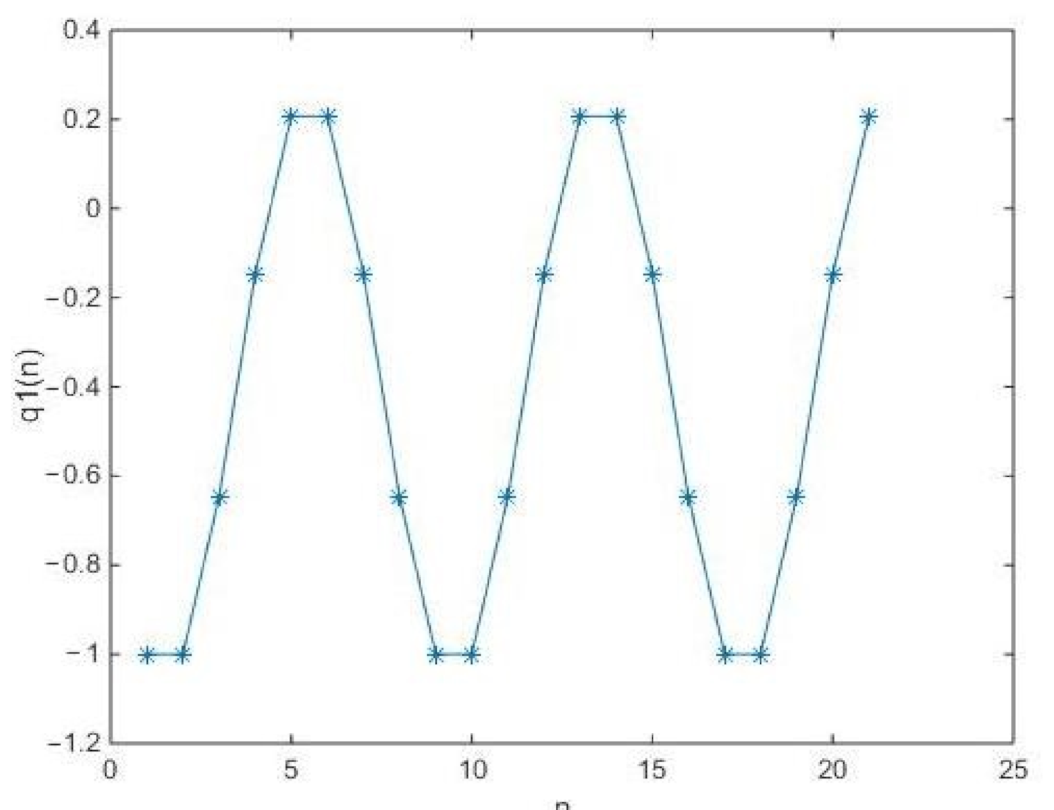
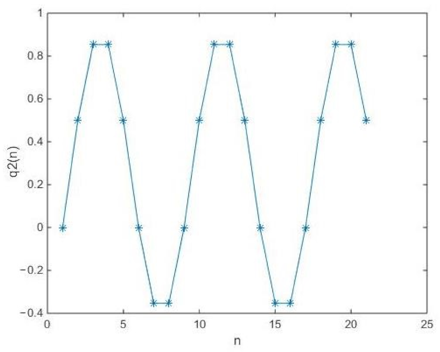
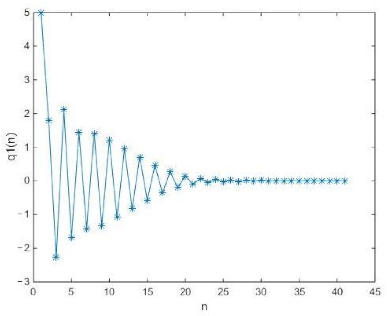
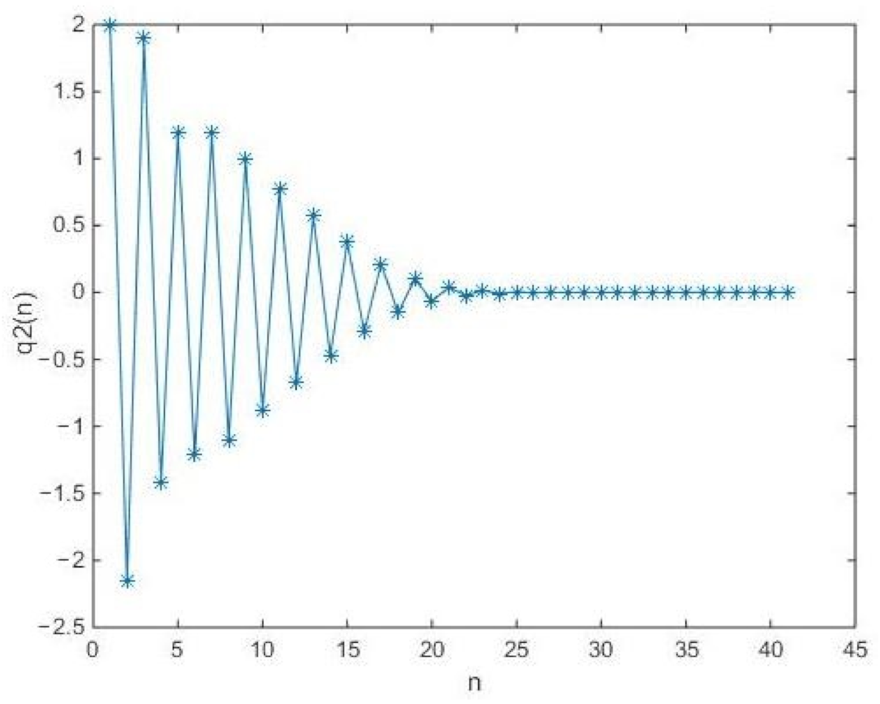
In what follows, we will provide two examples to support our obtained results of Theorem 8.

Example 1.

In Equation (4), let $s=1$, $x\left(s\right)={[q\left(1\right),q\left(2\right)]}^T$

$$B=C=\left[\begin{array}{cc}2& 0\\ 0& 2\end{array}\right],S\left(q\left(n\right)\right)=2q\left(n\right),f\left(n\right)= \left[\begin{array}{c}sin\frac{n\pi }{4}\\ cos\frac{n\pi }{2}\end{array}\right]q\left(1\right)= \left[\begin{array}{c}1\\ \frac{1}{2}\end{array}\right]q\left(2\right)= \left[\begin{array}{c}-1\\ 0\end{array}\right].$$

In fact,

$$B^{-1}= \left[\begin{array}{cc}\frac{1}{2}& 0\\ 0& \frac{1}{2}\end{array}\right],B^{-1}f\left(n\right)-B^{-1}S\left(q\left(n\right)\right)= \left[\begin{array}{c}\frac{1}{2}sin\frac{n\pi }{4}\\ \frac{1}{2}cos\frac{n\pi }{2}\end{array}\right]-q\left(n\right),R= \left[\begin{array}{cc}0& I\\ 0& I\end{array}\right],R^k=R.$$

Thus,

$$x\left(n\right)={[q\left(n\right),q(n+1)]}^T=Rx\left(s\right)+R\sum _{j=n-1-s}^{0}b(n-1-j),$$

and

$$q\left(n\right)= \left[\begin{array}{c}{q}_1\left(n\right)\\ q_2\left(n\right)\end{array}\right] = \left[\begin{array}{c}-1+{\displaystyle \sum _{j=n-1-s}^0}\frac{1}{2}sin\frac{(n-1-j)\pi }{4}\\ {\displaystyle \sum _{j=n-1-s}^0}\frac{1}{2}cos\frac{(n-1-j)\pi }{2}\end{array}\right].$$

For the status of $q_1\left(n\right)$ and $q_2\left(n\right)$, see Figure 1 and Figure 2.

Example 2.

In Equation (6), let $s=1$, $q\left(n\right)={[q_1\left(n\right),q_2\left(n\right)]}^T$, $q\left(1\right)={[1,1]}^T$, $q\left(2\right)={[5,2]}^T$, $\omega ={[0,1]}^T$

$$\begin{array}{cc}\hfill B\left(q\right(n\left)\right)=& C\left(q\left(n\right),q(n+1)-q\left(n\right)\right)\hfill \\ \hfill =& [2q\left(n\right),q\left(n\right)]+ \left[\begin{array}{cc}1& 0\\ 0& 0\end{array}\right]G\left(q\left(n\right)\right)= \left[\begin{array}{c}-q_2\left(n\right)cos\frac{n}{4\pi }\\ 1-q_{2}sin\frac{n}{8\pi }\end{array}\right].\hfill \end{array}$$

In fact,

$$\begin{array}{c}\hfill H\left(n\right)=H^k\left(n\right)= \left[\begin{array}{cc}0& I\\ 0& I\end{array}\right],L\omega = \left[\begin{array}{c}0\\ \frac{1}{2}\end{array}\right],\end{array}$$

$$\begin{array}{cc}\hfill B^{-1}\left(q\left(n\right)\right) = \left[\begin{array}{cc}1& \frac{-q_1\left(n\right)}{q_2\left(n\right)}\\ -\frac{1}{2}& \frac{sin\left(q_1\left(n\right)\right)-q_1\left(n\right)sin\frac{n}{8\pi }}{q_2\left(n\right)sin\frac{n}{8\pi }}\end{array}\right],L\omega -G\left(q\left(n\right)\right)=& \left[\begin{array}{c}{q}_2\left(n\right)cos\frac{n}{4\pi }\\ q_{2}sin\frac{n}{8\pi }\end{array}\right],\hfill \end{array}$$

$$\begin{array}{c}\hfill B^{-1}\left(q\left(n\right)\right)\left(L\omega -G\left(q\right(n\left)\right)\right) = \left[\begin{array}{c}{q}_2\left(n\right)cos\frac{n}{4\pi }-q_1\left(n\right)sin\frac{n}{8\pi }\\ -\frac{q_2\left(n\right)}{2}cos\frac{n}{4\pi }+sin\left(q_1\left(n\right)\right)-q_1\left(n\right)sin\frac{n}{8\pi }\end{array}\right].\end{array}$$

Hence,

$$\begin{array}{cc}\hfill x\left(n\right)=& \left(\prod _{j=s}^{n-1}H\left(j\right)\right)x_0+\sum _{j=s}^{n-2}\left[\prod _{i=1}^{n-(j+1)}H(n-i)\right]a\left(j\right)+a(n-1)\hfill \\ \hfill =& H(n-1)x_0+\sum _{j=s}^{n-2}H(n-i)a\left(j\right)+a(n-1)\hfill \end{array}$$

and

$$\begin{array}{cc}\hfill q(n+1)& =q\left(2\right)+{\displaystyle \sum _{j=1}^{n-2}}\left[\begin{array}{c}{q}_2\left(j\right)cos\frac{j}{4\pi }-q_1\left(j\right)sin\frac{j}{8\pi }\\ -\frac{q_2\left(j\right)}{2}cos\frac{j}{4\pi }+sin\left(q_1\left(j\right)\right)-q_1\left(j\right)sin\frac{j}{8\pi }\end{array}\right]\hfill \\ \hfill & +\left[\begin{array}{c}{q}_2(n-1)cos\frac{n-1}{4\pi }-q_1(n-1)sin\frac{n-1}{8\pi }\\ -\frac{q_2(n-1)}{2}cos\frac{n-1}{4\pi }+sin\left(q_1\left(n\right)\right)-q_1(n-1)sin\frac{n-1}{8\pi }\end{array}\right]\hfill \\ \hfill & =q\left(n\right) + \left[\begin{array}{c}{q}_2(n-1)cos\frac{n-1}{4\pi }-q_1(n-1)sin\frac{n-1}{8\pi }\\ -\frac{q_2(n-1)}{2}cos\frac{n-1}{4\pi }+sin\left(q_1\left(n\right)\right)-q_1(n-1)sin\frac{n-1}{8\pi }\end{array}\right].\hfill \end{array}$$

For the status of $q_1\left(n\right)$ and $q_2\left(n\right)$, see Figure 3 and Figure 4.

4. Conclusions

Anti-periodic phenomena always appear in various fields related to engineering science and technology. Almost anti-periodic phenomena is a natural extension of anti-periodic phenomena whose dynamical behavior can be reflected by almost anti-periodic process.

As an important tool of description of discrete process with almost anti-periodic circulation in the fields of engineering, biological chemistry, and neural computation, etc., a notion of discrete almost anti-periodic process has been proposed in this paper. Indeed, for an arbitrary almost anti-periodic sequence, the relatively dense set can also be applied to depict their accurate definitions. In the literature [26], Wang et al. addressed some basic notions to introduce a series of notions of almost periodic process on different types of time scales; the most convenient and precise statement is to adopt an intersection of intervals and subsets of real lines to portray the relative density distributed on time scales. The set with such an intersection property is called a relatively dense set. Naturally, it can be also applied to precisely describe an almost anti-periodic process on time scales.

The relatively dense set of the time scale version is presented as follows:

Assume that $\mathcal{T}$ is a time scale with periodicity, i.e., there is a nonempty set $\Omega \backslash \mathbb{R}\setminus \left\{0\right\}$ such that $t+\gamma \in \mathcal{T}$ for all $t\in \mathcal{T}$ and $\gamma \in \Omega$. Now, a standard notion of relative density of a subset of $\mathbb{R}$ could be introduced.

A subset S of $\mathbb{R}$ is called a relatively dense set if and only if there is a positive number $\mathcal{L}$ such that ${[b,b+\mathcal{L}]}_{\mathcal{T}}\cap S\ne \varnothing$ for each $b\in \mathcal{T}$.

By using this basic notion, we can also address the notion of an almost anti-periodic process on time scales.

Let $\mathcal{M}(·)={\left[{\mu }_{ij}(·)\right]}_{N\times N}:\mathcal{T}\to {\mathbb{R}}^{N\times N}$ be a $N\times N$ matrix-valued discrete function and $\omega (·)={[{\omega }_1(·),\dots ,{\omega }_N(·)]}^T:\mathcal{T}\to {\mathbb{R}}^N$ be a N-dimensional vector-valued function; then, we define

$$\parallel \mathcal{M}\left(t\right)\parallel =\frac{1}{N^2}\sum _{j=1}^N\sum _{i=1}^N|{\mu }_{ij}\left(t\right)|,\parallel \omega \left(t\right)\parallel =\frac{1}{N}\sum _{j=1}^N\left|{\omega }_j\left(t\right)\right|.$$

If for $\forall \epsilon >0$, there exists a positive integer $l\left(\epsilon \right)$ such that

$$\mathcal{E}(\epsilon ,\mu ):= \left\{\tau \in \Omega : \parallel \omega (t+\tau )+\omega \left(t\right)\parallel <\epsilon \right\}$$

is relatively dense. Then, $\omega \left(t\right)$ is called the almost anti-periodic discrete process, and $\mathcal{E}(\epsilon ,\omega )$ is called the $\epsilon$-almost anti-period of $\omega \left(t\right)$. Similarly, $\mathcal{M}\left(t\right)$ is an almost anti-periodic $N\times N$ matrix-valued function if

$$\mathcal{E}(\epsilon ,\mathcal{M})= \left\{\tau \in \Omega : \parallel \mathcal{M}(t+\tau )+\mathcal{M}\left(t\right)\parallel <\epsilon \right\}$$

is relatively dense.

The results of this paper provide a new avenue to study almost the anti-periodic process on a discrete time case. Meanwhile, the definition mode of function adopted in the paper could be extended to combine continuous cases and other complex time variables. Their comprehensive definitions and properties based on more complicated time situations will be investigated in our future research.

References

1. Agarwal, R.P.; Bohner, M.; Wong, P.J.Y. Sturm-Liouville eigenvalue problems on time scales. Appl. Math. Comput. 1999, 99, 153–166. [Google Scholar] [CrossRef]
2. Agarwal, R.P.; Meehan, M.; O’Regan, D. Fixed Point Theory and Applications, Cambridge Tracts in Mathematics, 141; Cambridge University Press: Cambridge, UK, 2001. [Google Scholar]
3. Agarwal, R.P.; Meehan, M.; O’Regan, D.; Peterson, A. Dynamic equations on time scales: A survey. J. Comput. Appl. Math. 2002, 141, 1–26. [Google Scholar] [CrossRef] [Green Version]
4. Breunung, T. Existence of quasi-periodic reponse in quasi-periodically forced nonlinear mechanical systems. Nonlinear Dyn. 2021, 105, 1977–2004. [Google Scholar] [CrossRef]
5. Chen, Y. Anti-periodic solutions for semilinear evolution equations. J. Math. Anal. Appl. 2006, 315, 337–348. [Google Scholar] [CrossRef] [Green Version]
6. Dimbour, W.; Valmorin, V. Asymptotically anti-periodic solutions for a nonlinear differential equation with piecewise constant argument in a Banach space. Appl. Math. 2016, 7, 1726–1733. [Google Scholar] [CrossRef] [Green Version]
7. Elaydi, S.N. An Introduction to Difference Equations; Springer: New York, NY, USA, 1996. [Google Scholar]
8. Kostić, M. Almost Periodic and Almost Automorphic Type Solutions of Abstract Volterra Integro-Differential Equations; W. de Gruyter: Berlin, Germany, 2019. [Google Scholar]
9. Kostić, M. Existence of generalized almost periodic and asymptotic almost periodic solutions to abstract Volterra integro-differential equations. Electr. J. Diff. Equ. 2017, 239, 1–30. [Google Scholar]
10. Liu, J.; Song, X.; Zhang, L. Existence of anti-periodic mild solutions to semilinear nonautonomous evolution equations. J. Math. Anal. Appl. 2015, 425, 295–306. [Google Scholar] [CrossRef]
11. N’Guérékata, G.M.; Valmorin, V.S. Anti-periodic solutions of semilinear integrodifferential equations in Banach spaces. Appl. Math. Comput. 2012, 218, 1118–1124. [Google Scholar]
12. Wang, C.; Agarwal, R.P. Almost periodic solution for a new type of neutral impulsive stochastic Lasota-Wazewska timescale model. Appl. Math. Lett. 2017, 70, 58–65. [Google Scholar] [CrossRef]
13. Wang, C.; Agarwal, R.P.; Sakthivel, R. Almost periodic oscillations for delay impulsive stochastic Nicholson’s blowflies timescale model. Comput. Appl. Math. 2018, 37, 3005–3026. [Google Scholar] [CrossRef]
14. Wang, C.; Agarwal, R.P. Almost automorphic functions on semigroups induced by complete-closed time scales and application to dynamic equations. Discret. Contin. Dyn. Syst. Ser. B 2020, 25, 781–798. [Google Scholar] [CrossRef] [Green Version]
15. Wang, C.; Agarwal, R.P. A classification of time scales and analysis of the general delays on time scales with applications. Math. Meth. Appl. Sci. 2016, 39, 1568–1590. [Google Scholar] [CrossRef]
16. Wang, C.; Agarwal, R.P. A survey of function analysis and applied dynamic equations on hybrid time scales. Entropy 2021, 23, 450. [Google Scholar] [CrossRef] [PubMed]
17. Wang, C.; Agarwal, R.P.; O’Regan, D. Local-periodic solutions for functional dynamic equations with infinite delay on changing-periodic time scales. Math. Slovaca. 2018, 68, 1397–1420. [Google Scholar] [CrossRef]
18. Wang, C.; Agarwal, R.P.; O’Regan, D. Matrix measure on time scales and almost periodic analysis of the impulsive Lasota-Wazewska model with patch structure and forced perturbations. Math. Meth. Appl. Sci. 2016, 39, 5651–5669. [Google Scholar] [CrossRef]
19. Wang, C.; Agarwal, R.P. Almost periodic dynamics for impulsive delay neural networks of a general type on almost periodic time scales. Commun. Nonlinear Sci. Numer. Simulat. 2016, 36, 238–251. [Google Scholar] [CrossRef]
20. Wang, C.; Agarwal, R.P. Uniformly rd-piecewise almost periodic functions with applications to the analysis of impulsive Δ-dynamic system on time scales. Appl. Math. Comput. 2015, 259, 271–292. [Google Scholar] [CrossRef]
21. Zhang, S.; Liu, P.; Gopalsamy, K. Almost periodic solutions of nonautonomous linear difference equations. Applic. Anal. 2014, 81, 281–301. [Google Scholar] [CrossRef]
22. Li, Z.; Wang, C.; Agarwal, R.P.; O’Regan, D. Commutativity of quaternion-matrix-valued functions and quaternion matrix dynamic equations on time scales. Stud. Appl. Math. 2021, 146, 139–210. [Google Scholar] [CrossRef]
23. Wang, C.; Agarwal, R.P.; O’Regan, D. Calculus of fuzzy vector-valued functions and almost periodic fuzzy vector-valued functions on time scales. Fuzzy Sets. Syst. 2019, 375, 1–52. [Google Scholar] [CrossRef]
24. Wang, C.; Li, Z.; Agarwal, R.P. Hyers-Ulam-Rassias stability of high-dimensional quaternion impulsive fuzzy dynamic equations on time scales. Discrt. Contin. Dynam. Syst. B 2022, 15, 359–386. [Google Scholar] [CrossRef]
25. Agarwal, R.P.; O’Regan, D. Some comments and notes on almost periodic functions and changing-periodic time scales. Electr. J. Math. Anal. Appl. 2018, 6, 125–136. [Google Scholar]
26. Wang, C.; Agarwal, R.P.; O’Regan, D.; Sakthivel, R. Theory of Translation Closedness for Time Scales, Developments in Mathematics; Springer: Cham, Switzerland, 2020; Volume 62. [Google Scholar]
27. Wang, C.; Agarwal, R.P.; O’Regan, D.; Sakthivel, R. A computation method of Hausdorff distance for translation time scales. Applic. Anal. 2020, 99, 1218–1247. [Google Scholar] [CrossRef]
28. Wang, C.; Agarwal, R.P.; O’Regan, D. Π-semigroup for invariant under translations time scales and abstract weighted pseudo almost periodic functions with applications. Dyna. Syst. Appl. 2016, 25, 1–28. [Google Scholar]
29. Wang, C.; Agarwal, R.P. Relatively dense sets, corrected uniformly almost periodic functions on time scales, and generalizations. Adv. Differ. Equ. 2015, 312, 1–9. [Google Scholar] [CrossRef]
30. Kostić, M.; Velinov, D. A notion on almost anti-periodic function in basic spaces. Kargujevac Math. J. 2020, 44, 287–297. [Google Scholar] [CrossRef]
31. Andrianov, I.V.; Awrejcewicz, J.; Danishevskyy, V.V. Linear and Nonlinear Waves in Microstructured Solids: Homogenization and Asymptotic Approaches; CRC Press: Boca Raton, FL, USA, 2021. [Google Scholar]
32. Craster, R.V.; Kaplunov, J.; Pichugin, A.V. High-frequency homogenization for periodic media. R. Soc. Math. Phys. Eng. Sci. 2010, 466, 2341–2362. [Google Scholar] [CrossRef] [Green Version]
33. Kostić, M.; Pilipović, S.; Velinov, D. Quasi-asymptotically almost periodic vector-valued generalized functions. Sarajevo J. Math. 2019, 15, 181–199. [Google Scholar]
34. Kostić, M. Asymptotically almost periodic and asymptotically almost automorphic vectorvalued generalized functions. Bul. Acad. Ştiinţe Repub. Mold. Mat. 2019, 3, 34–53. [Google Scholar]
35. Halmos, P.R. Finite-Dimensional Vector Spaces, Undergraduate Texts in Mathematics; Springer: New York, NY, USA, 1958. [Google Scholar]
36. Wang, Z.; Freidovich, L.B.; Zhang, H. Periodic motion planning and control for underactuated mechanical systems. Int. J. Control 2018, 91, 1350–1362. [Google Scholar] [CrossRef]
Figure 1. The status of the almost anti-periodic solution of the system (4).
Applsci 12 01991 g001
Figure 2. The status of the almost anti-periodic solution of the system (4).
Applsci 12 01991 g002
Figure 3. The status of the almost anti-periodic solution of the system (6).
Applsci 12 01991 g003
Figure 4. The status of the almost anti-periodic solution of the system (6).
Applsci 12 01991 g004
Publisher’s Note: MDPI stays neutral with regard to jurisdictional claims in published maps and institutional affiliations.