Article

Global Vibration Intensity Assessment Based on Vibration Source Localization on Construction Sites: Application to Vibratory Sheet Piling

Department of Civil and Environmental Engineering, The Hong Kong Polytechnic University, Hung Hom, Kowloon, Hong Kong 999077, China
*
Author to whom correspondence should be addressed.
Appl. Sci. 2022, 12(4), 1946; https://doi.org/10.3390/app12041946
Submission received: 26 December 2021 / Revised: 1 February 2022 / Accepted: 10 February 2022 / Published: 13 February 2022
(This article belongs to the Special Issue Advanced Numerical Simulations in Geotechnical Engineering)

Abstract

:
Various construction activities (such as piling) often generate high-intensity ground vibrations that adversely affect the surrounding environment. A common way of assessing vibration impact is to conduct on-site ground vibration monitoring at several selected locations. However, as vibration sources are often not pinpointed in the construction process, this approach cannot predict the vibration intensities at locations other than those monitored points. Therefore, the localization of vibration sources (e.g., vibratory sheet pile driving location) is crucial to quantify the corresponding vibration intensities in a broad area. This paper investigates a time-based source localization method based on wave propagation characteristics derived via three-dimensional finite element modeling of vibratory sheet pile driving in an infinite half-space soil domain. Satisfactory accuracy in the localization of the vibratory driving sources was achieved in all investigated numerical examples. Field validation tests were also conducted on a construction site with ongoing vibratory sheet pile driving work. A site-specific empirical formula was adopted to model the attenuation of measured vibration intensities with the increasing distance from the localized vibration source. As such, the combined utilization of the estimated vibration source location and the adopted empirical formula can achieve vibration intensity assessment in a broad surrounding area rather than being confined to a few monitored points.

1. Introduction

Construction activities such as pile driving frequently generate high-intensity ground vibrations that adversely affect surrounding environments. Numerous standards and specifications [1,2,3,4] define the allowable vibration limits of nearby objects, such as buried services, structures, people, and ultra-precision equipment. These limits are usually represented as peak particle velocity in the time domain or root mean square velocity in the frequency domain. Direct comparisons of vibration intensities with the allowable vibration limits are typically used to assess the impact of construction-related vibrations on nearby objects. Therefore, the prediction of ground vibration intensities due to common construction activities is a key part of such a vibration impact assessment procedure.
Various prediction models of ground vibration intensities have been developed in the literature. They can be categorized into three types, namely, empirical, theoretical, and engineering models [5]. Empirical models based on historical on-site measurements are often expressed in empirical formulas that describe how vibration intensity attenuates with distance from the vibration source [3,6,7,8]. Theoretical models are usually based on numerical and analytical modeling using various computer programs, in which complete dynamic responses of soil and/or structures during the process of common construction activities were simulated [9,10,11,12]. Engineering models often integrate the empirical, theoretical, and engineering knowledge to consider the dynamic characteristics of construction sites. For example, the past studies [13,14] focused on the derivation of the propagation function for vibration sources by performing seismic tests on a targeted construction site. Among these three categories, although theoretical and engineering models present higher reliability than empirical models, the former two also require more execution time and more sophisticated technical knowledge. Given that empirical models are comparatively simple to apply and require a small amount of input data, they are widely used to predict vibration intensities in real construction projects.
Empirical models are typically developed based on past field measurements, in which vibration intensities at different distances from vibration sources were measured by installing vibrometers at selected locations. According to the regression analyses of field measurement data, Wiss [7] suggested a simplified model:
PPV = k D n
PPV = K ( D E ) n
where PPV (mm/s) refers to the peak value of the resultant particle velocity, D (m) is the distance from the vibration source, k is the value of vibration amplitude at D = 1 m, E (J) is vibration source energy, D/E0.5 represents the scaled distance, K is the value of vibration amplitude at D/E0.5 = 1 (m/N)0.5, and n ranging from 1.0 to 2.0 refers to the attenuation rate exponent that accounts for both geometric and material damping. Site-specific vibration attenuation models can be developed by adopting Equation (1a). For example, Athanasopoulos and Pelekis [15] measured vibration intensity on ground surface points due to vibratory sheet pile driving with rated kinetic energy E = 1000–3000 J on different construction sites. Through the regression of data points, both mean values (n = 1.5, k = 32) and upper bound values (n = 1.5, k = 80) for Equation (1a) were suggested for the attenuation of ground vibration intensity along the distance. Zhu et al. [16] measured ground vibrations generated by vibratory sheet pile driving and rotary mini-pile driving. By using Equation (1a), they proposed the upper bounds of ground vibration intensity for vibratory sheet pile driving (n = 1.1, k = 43) and rotary mini-pile driving (n = 1.3, k = 12).
Based on their statistical analyses of recorded data, Attewell et al. [8] concluded that compared with a linear regression curve, a quadratic regression curve provides a better visual fit to the investigated data sets. They suggested using the quadratic one-half standard deviation curves as shown in Equation (2) for assessing ground vibrations from pile driving with impact hammers and vibrodrivers:
log PPV = p + m log ( E 0.5 / D ) + n log 2 ( E 0.5 / D )
where PPV (mm/s) also refers to the peak resultant particle velocity, and p, m, and n are constants of proportionality that are determined empirically.
Caltrans [3] suggested substituting the empirical vibration intensity factor (k, K, and p) in Equations (1) and (2) with the vibration intensity in a reference case, and proposed the following formula for predicting pile driver-generated vibrations:
PPV V i b r o = PPV r e f ( D D r e f ) n
PPV I m p a c t = PPV r e f ( D D r e f ) n × ( E e q u i p E r e f ) 0.5
where PPVVibro (mm/s) and PPVImpact (mm/s) represent the peak vertical velocity component, which is different from the definition of PPV in Equations (1) and (2) using the peak resultant particle velocity, produced by one vibratory pile driver and one impact pile driver, respectively; D (m) refers to the distance from a pile driver to a receiver; Eequip (J) represents the pile driver’s rated energy; and PPVref = 16.5 mm/s represents the reference peak vertical particle velocity at a distance of Dref = 7.6 m by a pile driver with rated energy of Eref = 48,806 J. The suggested value for the exponent n is 1.1, but it can vary from 1.0 to 1.4 to reflect different soil types.
Construction-induced vibrations must be inspected and controlled by following the criteria of safe vibration [17,18]. Many construction projects implement the practice of real-time construction vibration monitoring in a compulsive manner. After reviewing the worldwide standards and practices of noise and vibration monitoring on different construction sites, Manvell [19] concluded that the design of monitoring systems is affected by many factors such as criteria, assessment methodology, noise and vibration index, and means of display. To decide appropriate ground vibration monitoring distances in the process of pile driving, Zhang et al. [20] designed a statistical procedure to prevent possible construction-related damage. Lemke [21] developed a remote vibration monitoring system by using wireless internet data transmission to collect, process, transmit, and analyze vibration measurement data obtained on construction sites. Veggeberg [22] designed a wireless noise and vibration management system to meet the standards set by the local regulations. Meng and Zhu [23] built a wireless Internet of Things sensing system to conduct the real-time monitoring and assessment of construction-induced vibrations.
However, several limitations in the current construction-induced vibration impact assessment practice are worth further attention. First, by assuming construction scenarios (e.g., construction locations and methods) prior to real construction work, the aforementioned empirical models are typically applied to predict vibration intensities in a large area. Such prediction measures lead to great limitations in construction operations and also are often inaccurate given the great variability in construction-related vibrations. Second, the real-time global vibration impact assessment based on the empirical models is often prevented by moving vibration sources with their exact locations unknown in construction processes. Considering its unavoidable delay and inefficiency, the manual input of locations by construction workers is undesirable in an automatic process of vibration monitoring and assessment. Third, real-time vibration monitoring on construction sites can only guarantee a local vibration impact assessment because the selected monitoring points in reality usually cannot cover the whole surrounding area due to budget limitations. In this case, purely relying on a large number of vibration monitoring points is not a cost-effective solution to realize global vibration impact assessment.
Therefore, how to conduct real-time vibration intensity assessment over the entire construction site rather than at several discrete monitoring points remains challenging. In this study, we combine the empirical formulas with the localization of vibratory pile driving to address this issue. We draw upon the concept and methodology proposed by Wang and Zhu [24], who attempted to localize the unknown impact source on construction sites by using the time of arrival (ToA) of impact waves recorded by transducers and the coordinates of these transducers. However, whether this localization method derived from the simulations of an impact source can be extended to other vibration sources remains unknown at present. For example, an impact source and a vibratory pile driving source correspond to different wave generation mechanisms and wave propagation characteristics. Moreover, ground wave propagations and source localization performances are affected by multiple influencing factors, which have not been considered in the literature [24].
Therefore, in this study, we investigate the time-based localization method to localize a vibratory pile driving source on construction sites and subsequently realize a global prediction of vibration intensities over a broad area. The transient finite element analysis was performed to simulate the wave propagation from one vibratory sheet pile driving source to the far-field in an infinite half-space soil domain, on which the time-based localization method for vibratory driving source was based. The effects of the layout of monitoring points, pile toe depths, ground conditions, vibratory driving frequencies, and pile–soil friction coefficients on the localization performance were systematically investigated through numerical simulations. Field validation tests were performed on a construction site with vibratory sheet pile driving work under construction. Finally, a site-specific empirical formula was adopted to predict vibration intensities at different distances from the localized vibratory driving source.

2. Numerical Simulations of Vibratory Sheet Pile Driving

2.1. Simulation Model

As displayed in Figure 1, a full-scale finite element (FE) model was established using the commercial ABAQUS software. The model consisted of two parts—the soil domain and the sheet pile pre-inserted in the soil domain. The simulated soil domain was 120 m × 120 m × 100 m (X × Y × Z). The element type selected for soil was C3D8R, eight-node quadrilateral elements with reduced integration and hourglass control. At the four surrounding sides, the external soil domain with 30 m was modeled and discretized into infinite elements (CIN3D8), which are typically used to model non-reflective boundaries to transmit energy outside the mesh boundaries (Figure 1b). In the vertical direction, a large depth of 100 m was modeled, which is enough to avoid wave reflections from the bottom side of the model.
Element dimensions should be selected on the basis of the highest frequency fmax and the lowest wave velocity vr [25]. A rational element dimension g is determined by:
g χ v r f max
where the constant χ must be less than 0.5 due to the Nyquist limit, and it is further determined by whether the mass matrices are consistent (χ = 0.25) or lumped (χ = 0.2). Thus, according to the simulated soil properties and vibratory driving frequency, a uniform mesh size of 0.35 m was used in three directions of the soil domain, except for soil elements near the pile axis, where a finer mesh size was defined to guarantee suitable contact between pile and soil.
For simplicity, in this study, we assumed the sheet pile as a medium only to transmit the vibratory driving force to the surrounding soil through the pile toe force and the shaft friction. Consequently, the sheet pile was modeled as a discrete rigid body whose motion was governed by a pre-defined rigid body reference node [26]. The pre-defined reference node was assigned with the total mass of the sheet pile, which was calculated according to its geometry and material properties defined in Table 1, wherein the modeled sheet pile has a standard U-type section supplied by a local corporation in Hong Kong and follows the specification of BS EN 10248:1996 [27]. Soil domain was typically modeled as a homogeneously elastic–plastic medium using the Mohr–Coulomb model to consider the nonlinear behavior of soil in the vicinity of the pile. As listed in Table 2, we adopted the same soil parameters as those used in previous studies [10,11,12] to define the soil behavior. It should be noted that the modeled soil properties correspond to a shear wave velocity consistent with the tested construction site presented in Section 4. In addition, an appropriate material damping ratio of 7% was defined to consider the anelastic property of soil.
The surface-to-surface contact discretization formulation in ABAQUS was used to define the interaction between sheet pile and soil, wherein the normal and tangential behavior were simulated using the hard contact model and the Coulomb friction model, respectively. The friction coefficient was set as μ = 0.25 for the steel sheet piles against silty sand, gravel, or sand mixed with silt or clay, according to NAVFAC standards [28].
The loading procedure consists of two steps. In the first step, gravity was added to the whole pile–soil system to establish an initial stress state of the whole soil domain and contact state between pile and soil. In the second step, a vibratory driving force was applied to the pre-defined rigid body reference node of the pile to generate the spatial vibration propagations in the soil. This study adopted the driving force Fp(t) = 800sin(2πf0t) + 100 kN, which was suggested in [10] for a standard hydraulic vibratory driver ICE 44–30V operating at a frequency f0 = 20 Hz with an eccentric moment me = 50.7 kg·m. To save computational time, the duration of driving force was defined as 0.5 s only, while the total duration of the analysis steps was defined as 1.2 s so that the generated vibrations could propagate across the whole soil domain.
The Abaqus/Explicit dynamic analysis was used for the calculations since it is efficient in calculating large models with short dynamic response times. The explicit procedure adopts a conditionally-stable central-difference time integration rule. The time increment steps were automatically selected by ABAQUS during the analysis in this study.

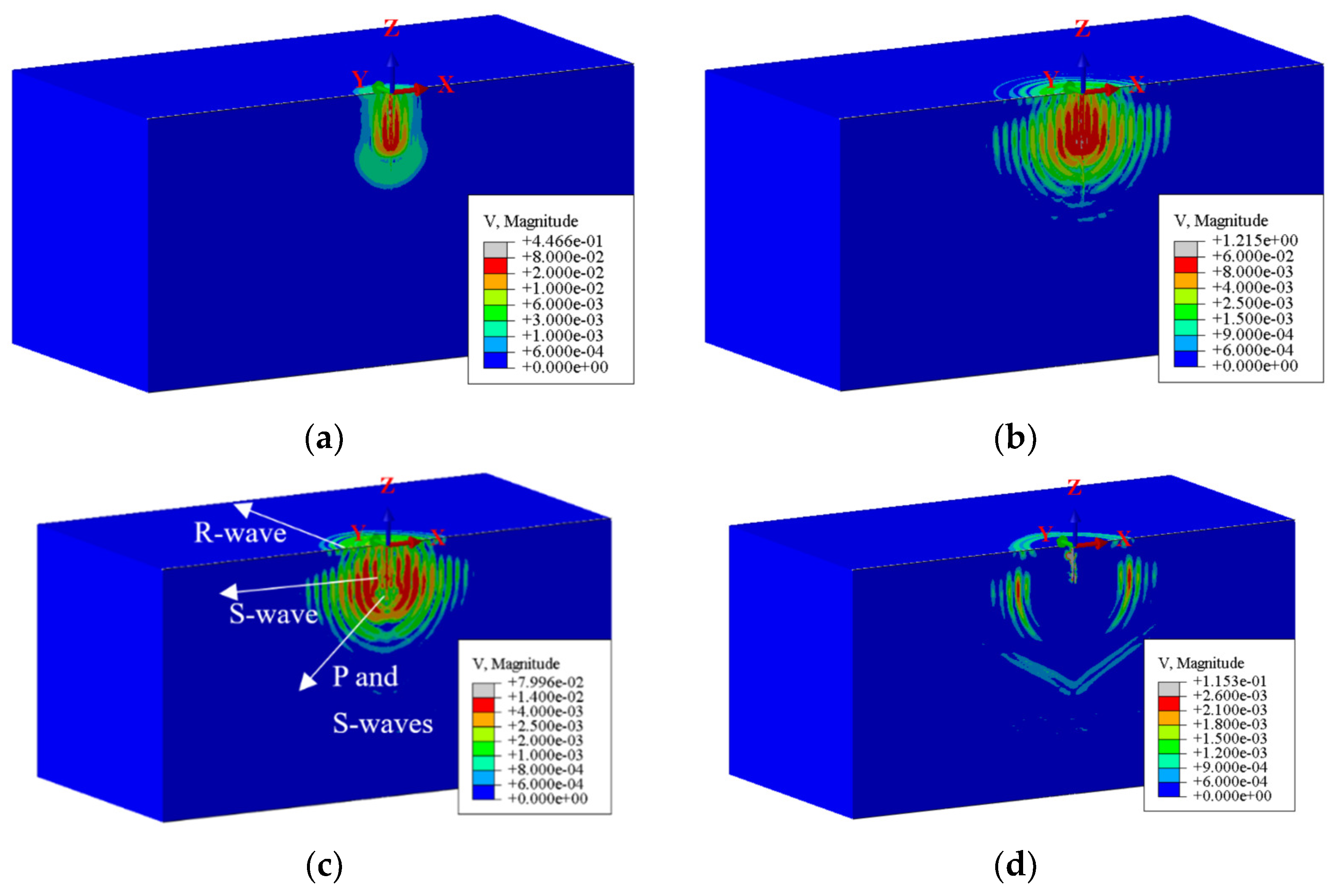
2.2. Numerical Simulation Results

Based on the model described above, spatial wave propagations due to vibratory sheet pile driving at different depths were simulated. Figure 2 displays a representative example of wave propagations when the pile toe is located at 10 m below the ground surface. The snapshots at time steps t = 50 ms (i.e., one period after the start of the driving force), t = 300 ms (i.e., six periods after the start of the driving force), t = 550 ms (i.e., one period after the end of driving source), and t = 700 ms (i.e., four periods after the end of driving source) are presented. These snapshots show that three types of wavefronts emerged as the wave propagated away from the vibratory driving location. Because of the cyclic dynamic frictions between pile shaft and adjacent soil, cylindrical wavefronts of shear wave (S wave) with the largest amplitude are generated from the pile shaft ranging from the ground surface to the pile toe. Similarly, due to the cyclic dynamic contact force between the pile toe and the underlying soil, spherical wavefronts of body waves (P and S waves) are generated from the pile toe. There are also cylindrical wavefronts of surface wave (R wave) near the ground surface, which is always slower than the cylindrical wavefronts generated by the pile shaft. The surface waves are formed through the interaction between the reflected body waves and advancing shear waves near the ground surface [29,30]. Similar observations of wave propagations were made when pre-embedding the pile toe at other depths.
Vibration responses of pile and soil nodes were subsequently investigated. Figure 3 shows the adopted spatial Cartesian coordinate system and definitions of plan distance d and radial distance r, which help position the investigated soil nodes on and below the ground surface.
Figure 4 displays the vertical velocity time histories of the pile and three soil nodes at different depths (Z = 0, −7, −25 m) but the same plan distance (d = 20 m). The ToA between the pile vibration and soil vibrations can be observed. The cross-correlation function is widely used to determine the time lag between two discrete vibration signals in the time domain. The mathematic form is represented as:
( f g ) [ n ] m = f [ m ] ¯ g [ m + n ]
in which f and g represent two discrete vibration signals and f [ m ] ¯ is the complex conjugate of f [m], and n is the time lag indicating that a feature in f at m occurs in g at m + n. Therefore, the time lags n (i.e., ToAs) in Equation (5) for vibration signals at any soil nodes were computed by performing a cross-correlation function between the vibration signal of the pile and corresponding vibration signals of soil nodes.
The ToAs at different ground surface points on the X-Y plane (0 < X < 50 m, −50 m < Y < 50 m and Z = 0) and underground points on the X-Z plane (0 < X < 50 m, Y = 0 and −30 m < Z < −3 m) were collected. To differentiate the wave types based on wave travel velocities, the relationships between the collected ToAs and wave travel distance are illustrated in Figure 5. Specifically, Figure 5a shows the ToA’s variation at the ground surface points (Z = 0) along with the plan distance from the pile shaft, Figure 5b shows the ToA’s variation of underground points within the depth of the pile shaft (−10 m < Z < −3 m) along with the plan distance from pile shaft, and Figure 5c shows the ToA’s variation of underground points below the pile toe (−30 m < Z < −10 m) along with the radial distance r from pile toe. The wave velocities of R wave (vr = 111 m/s), S wave (vs = 120 m/s), and P wave (vp = 293 m/s), which were computed based on elastic parameters of soil, are also illustrated in Figure 5. The comparison in Figure 5a indicates that the vibrations experienced by ground surface points (Z = 0) represent the R wave, and the comparison in Figure 5b indicates that the vibrations experienced by underground points within the depth of the pile shaft (−10 m < Z < −3 m) represent the S wave from the pile shaft, whereas the comparison in Figure 5c reveals that the vibrations experienced by underground points below the pile toe (−30 m < Z < −10 m) represent two wave types from the pile toe: S wave and P wave.
Figure 6 displays the particle motions of soil nodes at different plan distances (d = 5, 20, and 40 m) and depths (Z = 0, −7, −25 m) on the X-Z plane. It can be observed that the particle motions of the three ground surface points (Z = 0 m) display retrograde elliptical shapes and the vertical magnitude of motion is greater than the horizontal one, which is a typical characteristic of R wave. The particle motions of the three underground points (Z = −7 m) take place predominantly in the vertical direction, which presents the feature of cylindrical S wave from the pile shaft. The particle motions of the three underground points (Z = −25 m) display two nearly orthogonal directions, wherein particle motions induced by P and S waves from pile toe are parallel and perpendicular to the direction of wave propagation, respectively.

3. Time-Based Localization Method and Localization Performance in Numerical Examples

3.1. Time-Based Localization Method

Based on wave propagation characteristics analyzed in the previous section, the time-based localization method is proposed. We focused on the monitoring points deployed on the ground surface (X-Y plane) where the propagation of a single surface wave (R wave) was assumed due to the vibratory driving source on a construction site. The difference in wave arrival time (ΔToA) between two monitoring points can be presented as:
( x x i ) 2 + ( y y i ) 2 ( x x j ) 2 + ( y y j ) 2 v r = t i j
where tij represents the ΔToA between the ith monitoring point Pi (xi, yi) and the jth monitoring point Pj (xj, yj), x and y are unknown coordinates of the vibratory driving source, and vr refers to the surface wave velocity. Similar relationships can be built among other monitoring points. The coordinate of the vibratory driving source (x, y) can be calculated by solving these nonlinear equations considering the known coordinates of monitoring points and ΔToAs among them, without knowing the wave velocity. This study adopts the optimization function, fsolve function in MATLAB [31], for the optimization calculations and the cross-correlation function (Equation (5)) for the determination of ΔToA (tij) among multiple monitoring points.
Once the vibratory driving source is localized, the measured vibration intensities at estimated plan distances to the localized driving source can be utilized to develop a site-specific empirical prediction model. As such, a global vibration intensity assessment can be achieved on the entire construction site.

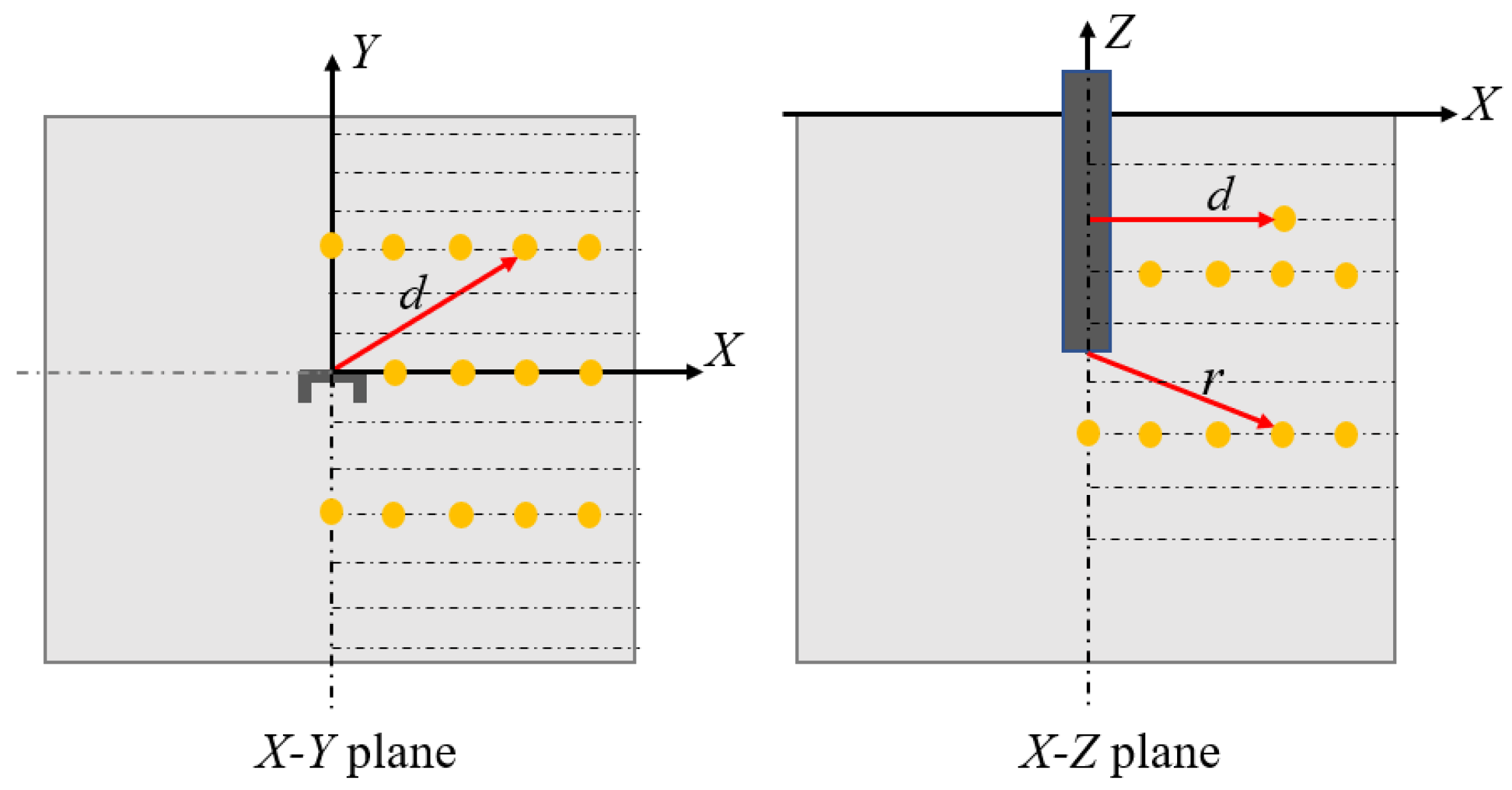
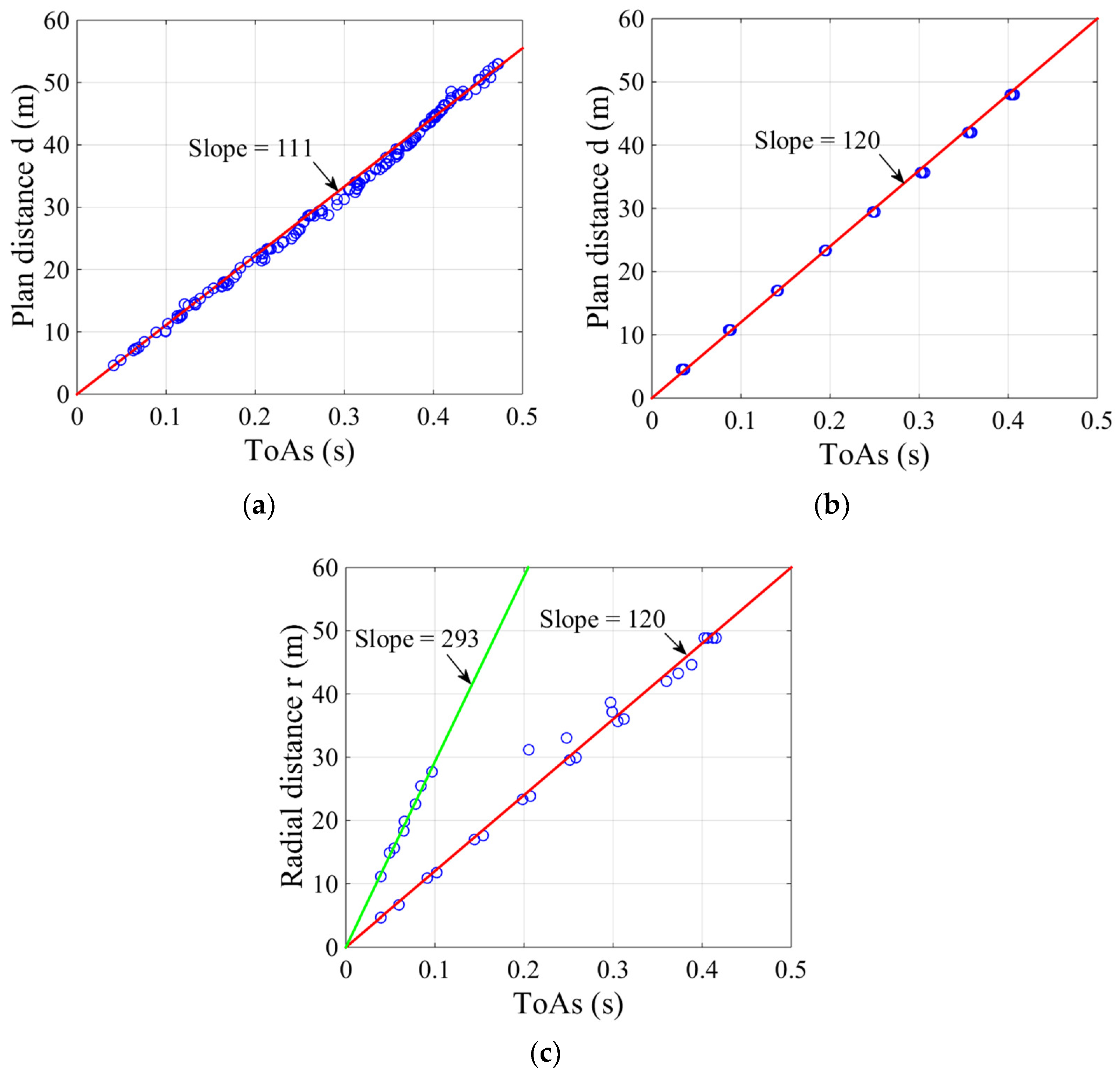
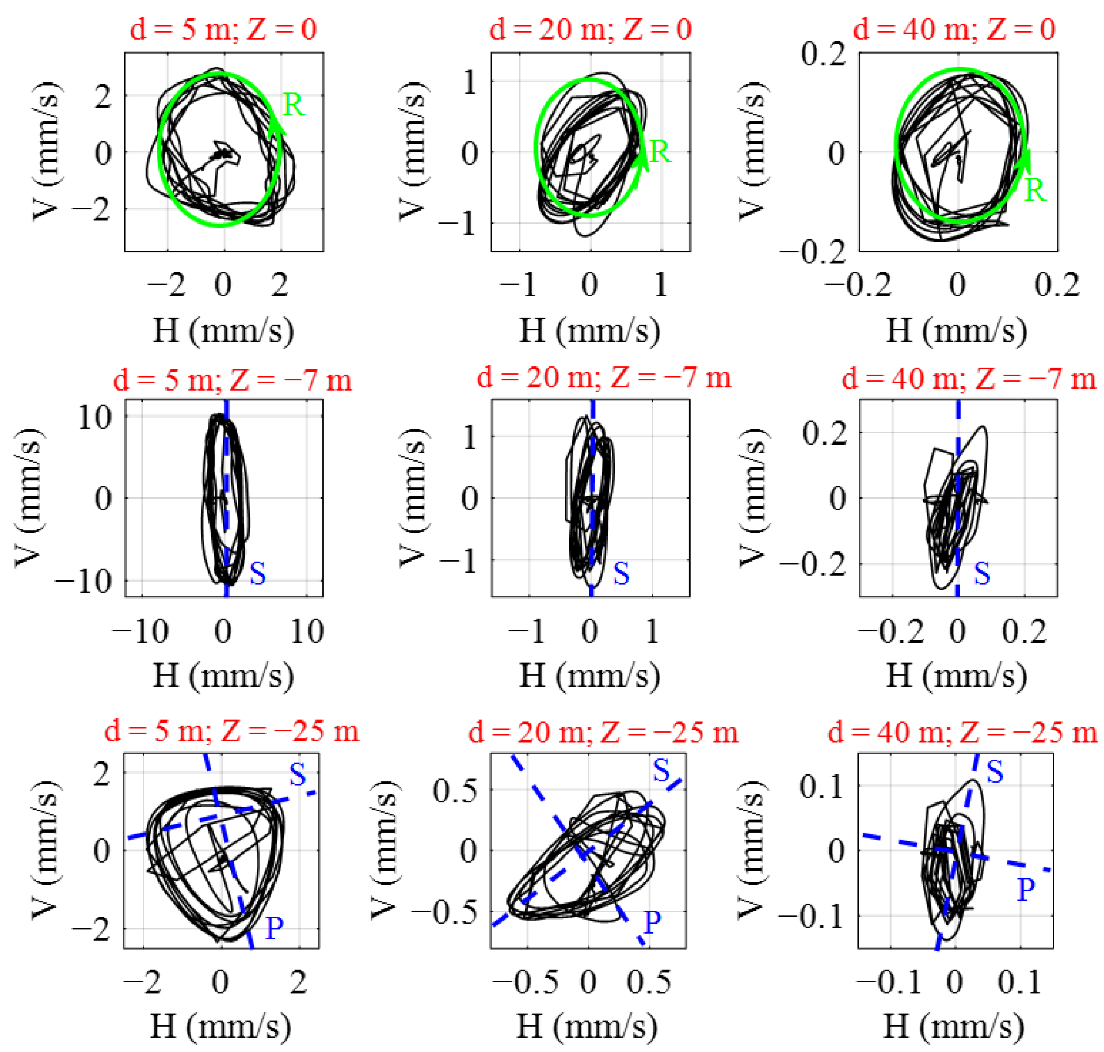
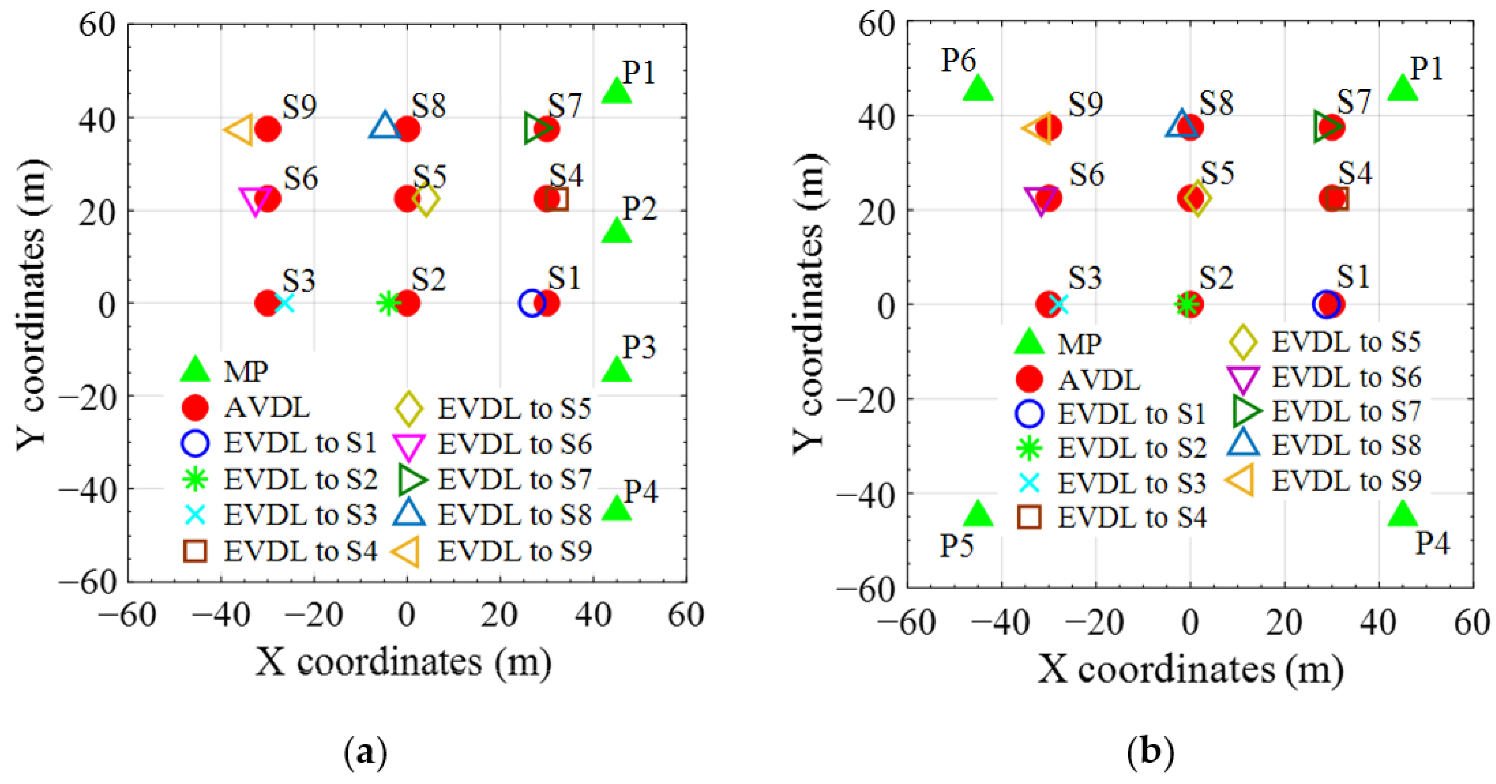
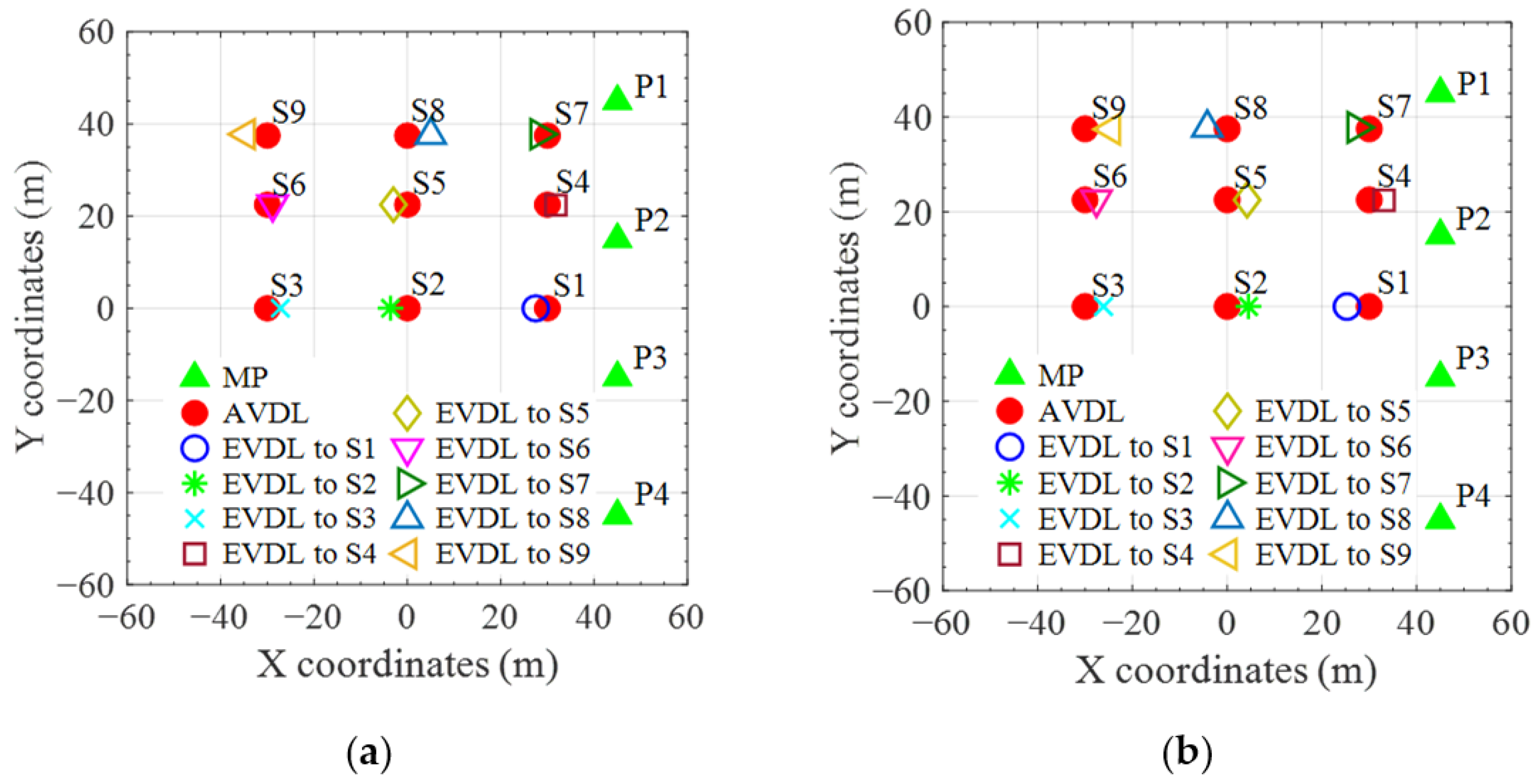
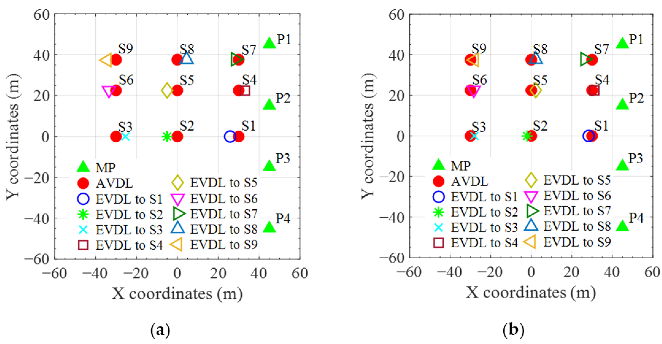
3.2. Localization Performance in Numerical Examples

Numerical simulations were conducted to verify the proposed time-based localization method. It begins with the investigation of the effects of actual pile toe depths and spatial relationships between monitoring points and driving locations on localization performance. Figure 7 shows the ground surface (i.e., X-Y plane) of the simulated soil domain. A total of nine vibratory sheet pile driving locations (S1 to S9) and two pile toe depths (i.e., the ground surface and 10 m below ground surface) at each location were modeled. Linear and square layouts of monitoring points were deployed on the ground surface to model different deployment cases on construction sites, wherein the distances between two adjacent monitoring points were set as 30 m and 90 m in the linear and square layouts, respectively. A constant sampling interval was set as 0.001 s (i.e., a sampling frequency of 1 kHz) in the simulated velocity signals. After vibratory driving-induced velocity signals were collected at the deployed monitoring points, localizations of those tested source locations were performed according to the time-based localization method proposed in this study.
Figure 8 displays the localization results when the vibratory sheet pile driving takes place on the ground surface. Monitoring points in the linear sensor layout were used for the localization. As observed from Figure 8, deviations exist between the estimated and actual vibratory driving locations due to the possible inconsistent wave propagation velocities among monitoring points. Such inconsistency in wave propagation velocities can be induced by the interference of body waves, given that the single type of surface wave is pre-assumed to propagate along the ground surface. The relative errors were defined as the ratio of estimation errors in the coordinates (x, y) to the site dimension (i.e., 120 m in both directions in numerical examples). Table 3 shows the calculated relative errors for different vibratory driving locations (S1 to S9). The relative error ranges from 0.92% to 2.08% in the X direction and from 0.02% to 0.19% in the Y direction. Generally, the localization accuracy in the Y direction was better than that in the X direction because the used monitoring points were aligned in the Y direction.
Figure 9 displays the localization of the plane coordinates when the pile toe is pre-embedded 10 m below the ground surface. The localization results derived by using monitoring points in the linear and square layouts were displayed. It can be observed that a much better localization accuracy is achieved by using the monitoring points in the square layout. As also listed in Table 3, the mean relative error decreases from 2.69% in the linear layout to 1.28% in the square layout, and the maximum relative error decreases from 4.00% in the linear layout to 1.75% in the square layout. It can be concluded that spatial relationships have a great impact on localization performance. The layout of monitoring points spreading in both directions and surrounding the driving locations can improve the localization performance compared with the layout of monitoring points deployed along a single direction. Moreover, because of the more complex wave types and paths generated when the pile toe is in deep positions, a higher degree of inconsistency in wave propagation velocity was expected among the investigated monitoring points, which degraded the localization accuracy compared with those cases when the pile toe is placed on the ground surface.
The sensitivity studies were conducted to investigate the localization performance due to the changes in the ground shear wave velocity, the vibratory driving frequency, and the friction coefficient at the pile–soil interface when the pile toe is pre-embedded 10 m below the ground surface and the monitoring points in the linear layout are utilized.
Compared with the localization results shown in Figure 9a for the simulation case: the shear wave velocity vs = 120 m/s, driving frequency f0 = 20 Hz, and friction coefficient μ = 0.25, Figure 10 presents the localization results of plane coordinates for two other shear wave velocities (vs = 60 m/s and 250 m/s), Figure 11 shows two other driving frequencies (f0 = 40 Hz and 60 Hz), and Figure 12 displays two other friction coefficients (μ = 0.1 and 0.4). Overall, the localized driving source is reasonably close to the actual driving locations in these figures. The localized deviations are mainly reflected in the X direction due to the monitoring points aligned in the Y direction.
Table 4 presents the mean and maximum relative errors in sensitivity studies. When considering the larger driving frequency and shear wave velocity, the adopted constant sampling rate (i.e., 1 kHz) cannot guarantee enough accuracy in ΔToAs among monitoring points. As shown in Table 4, either a larger shear wave velocity or higher driving frequency can induce a slight increase in the relative errors of the estimated coordinates. For example, the mean relative error (X direction) increases by 0.87% when vs changes from 120 m/s to 250 m/s, and it increases by 1.04% when f0 changes from 20 Hz to 60 Hz.
The relative errors can also be affected by the change in the pile–soil friction coefficient, which might be explained by the generated wave contents during the pile–soil interactions. As discussed before, the body waves generated from the pile toe influence the localization accuracy by complicating the collected velocity signals. As the friction coefficient decreases, the percentage of body waves generated from the pile toe increases, and their adverse effects on the localization performance are magnified. For example, the mean relative error (X direction) increases by 0.66% when the friction coefficient μ decreases from 0.25 to 0.1.
Notably, among all numerical examples, the maximum values of the mean and maximum relative errors (X direction) are 3.73% and 5.30%, respectively. Consequently, it proves, to some extent, the applicability of the proposed localization method in different ground and construction conditions.

4. Field Validation Tests and Global Vibration Intensity Prediction

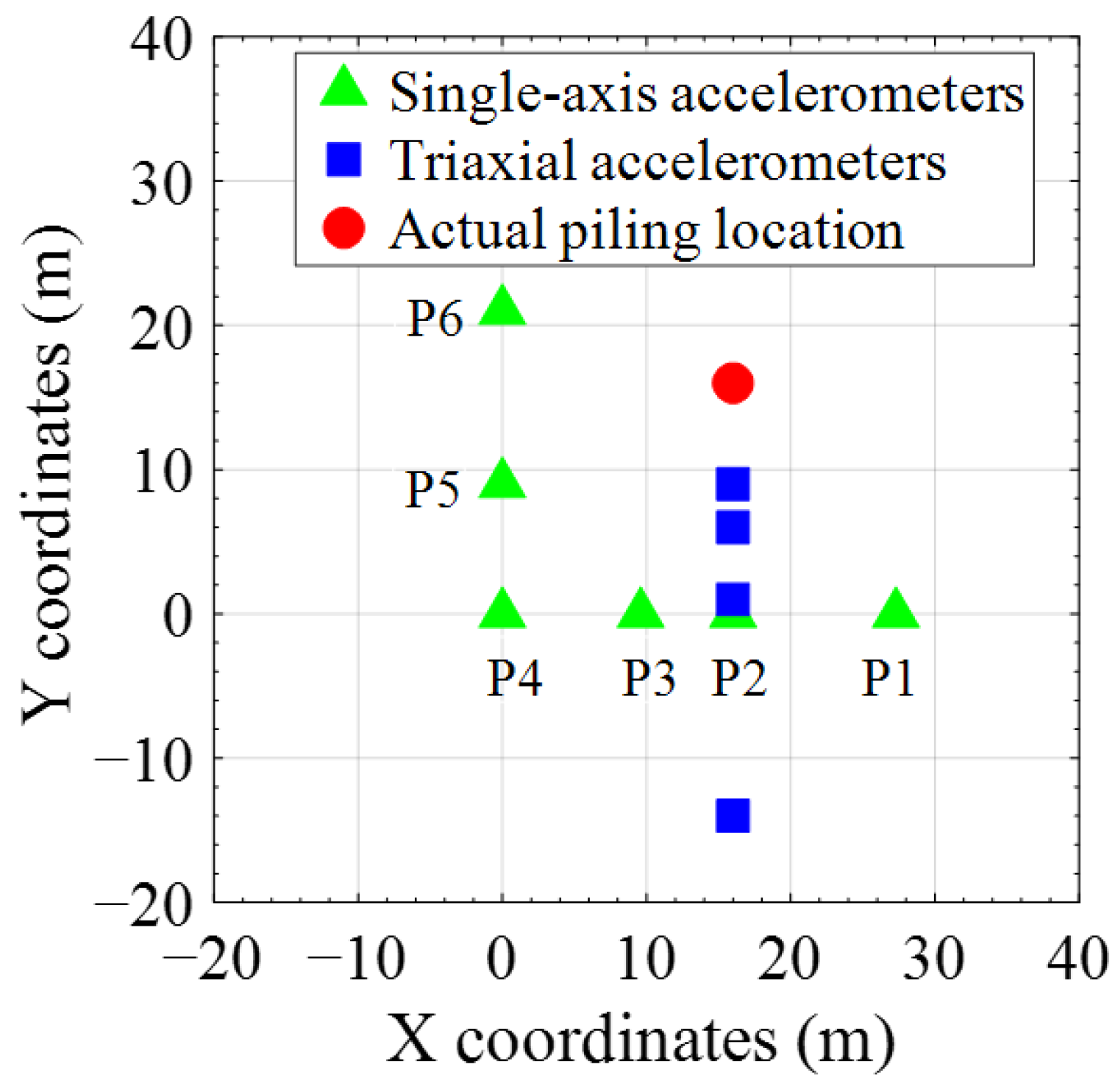
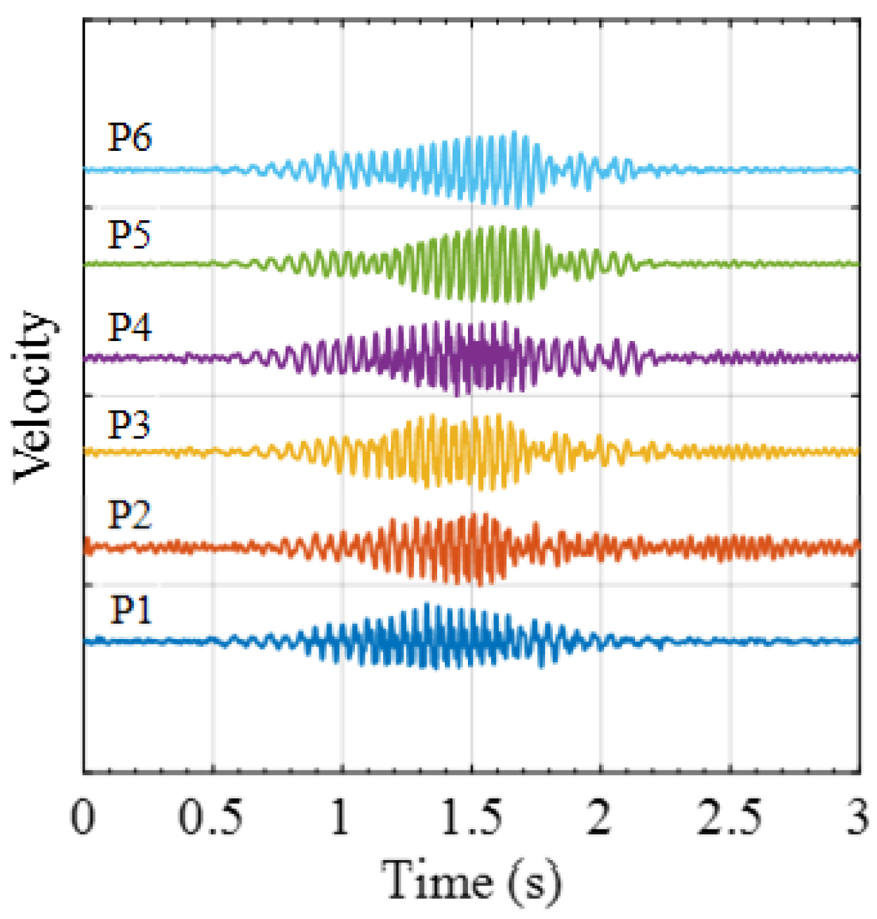
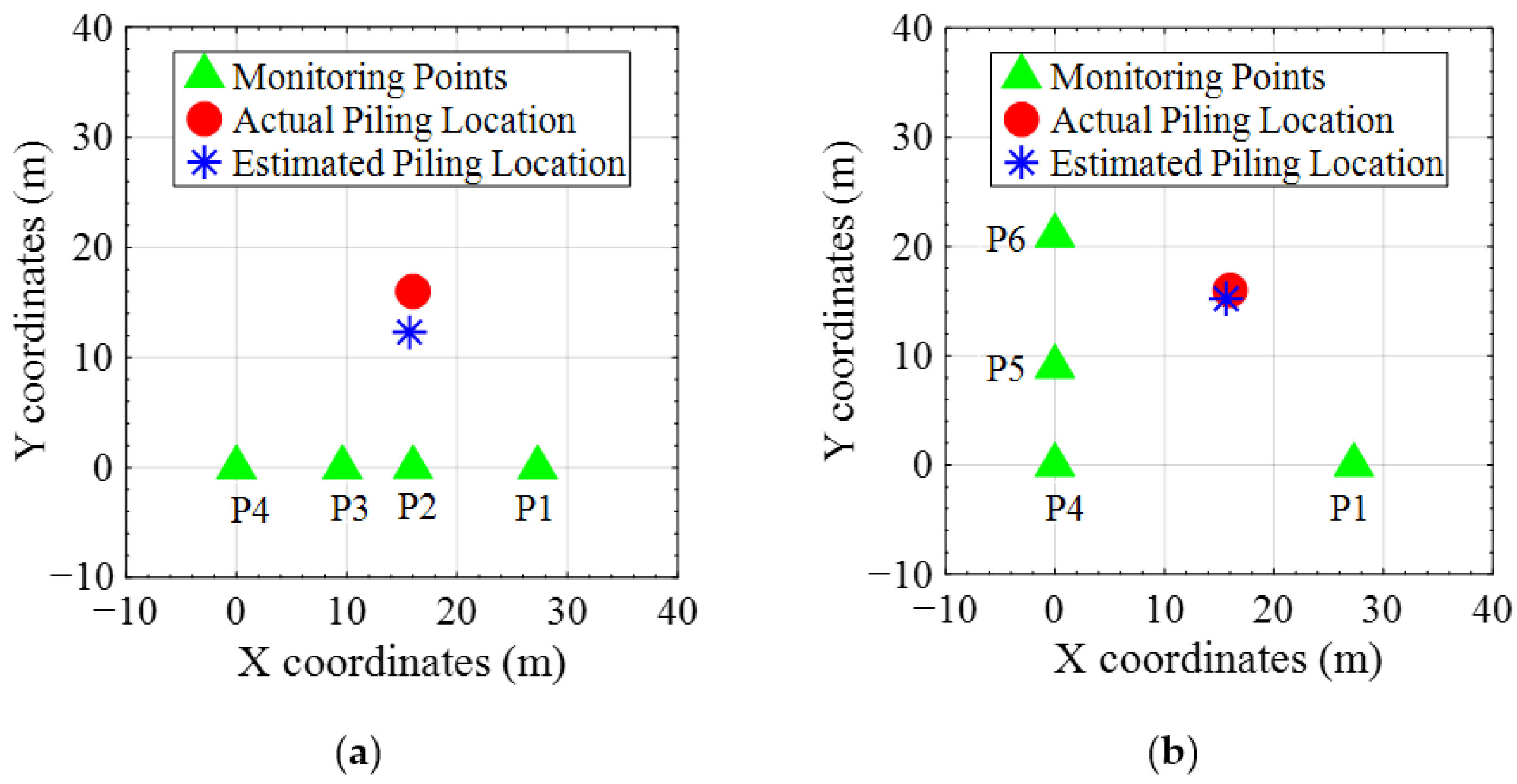
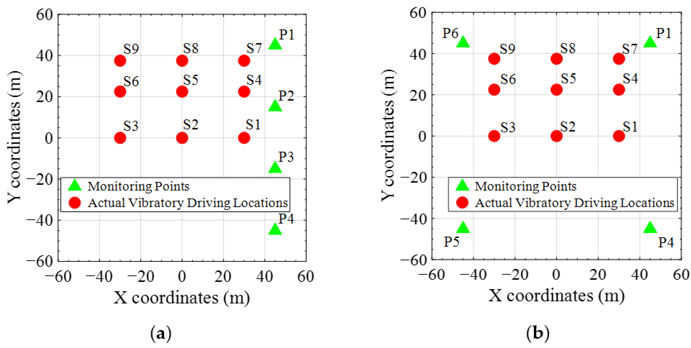
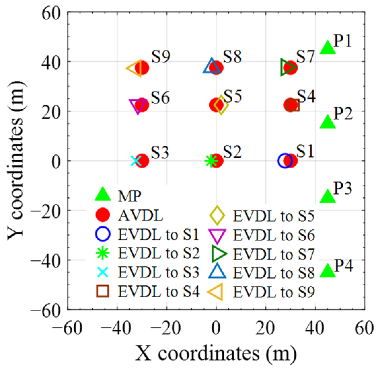
4.1. Field Validation Tests

Field validation tests were conducted on a construction site with ongoing vibratory sheet pile driving works. Figure 13a displays the photo of the selected construction site in Hong Kong. The ground investigation report indicated that the equivalent shear wave velocity was around 100 m/s. Figure 13b shows the steel sheet pile with a length of 6 m, and the pile head was driven by a commercial excavator-mounted vibratory hammer that operated at a frequency f0 = 20 Hz with an eccentric moment me = 7.5 kg·m. Two sets of vibration data acquisition systems were used during the measurement. Figure 13c shows the first set of vibration data acquisition systems (model #: NI USB-6343 BNC), which comprised six uniaxial accelerometers (model #: KD 1000) to simultaneously collect vertical vibration signals at a sampling frequency of 1 kHz. The installation of one accelerometer on the ground surface is shown in Figure 13d: a steel soil nail was first knocked into the soil at the selected monitoring point, and the accelerometer was then attached to the block surface of the soil nail by using strong magnets. Figure 13e shows the second set of vibration data acquisition systems, which is a portable three-channel C-series dynamic signal acquisition module (model #: NI 9230). By using the same installation method, triaxial accelerometers (model #: 356 B18), as shown in Figure 13f, were used to measure vibration signals in three orthogonal directions.
Figure 14 shows the layout of the ten selected monitoring points (six points with uniaxial accelerometers and four points with triaxial accelerometers) deployed on the ground surface. By using two sets of monitoring systems, the complete vibratory driving process (from the ground surface to 6 m depth) for one sheet pile was measured.
The following particle vibration trajectories, vibration histories, and PPV values are presented based on the velocity signals, which were computed by using filters and performing one-time integration of the measured acceleration time histories. Using velocity can reduce the amplification of high frequencies compared with using acceleration and avoid the accumulated error of double integration when using displacement [32].
To investigate the wave type of measured vibration signals, particle vibration trajectories at a plan distance of d = 15 m measured by one triaxial accelerometer are plotted in Figure 15 by combining the vertical (i.e., V) and two horizontal (i.e., H1 (or Y) and H2 (or X)) time histories of motions. The particle motion occurs mainly in the radial vertical plane (H1-V) with an elliptical shape and the vertical magnitude of motion is greater than the horizontal one. These observations reflect the characteristics of R waves propagating near the ground surface.
Vibration measurement results at the six points (P1–P6) by single-axis accelerometers were used to localize the vibratory driving location. Figure 16 shows the adopted segments of vibration signals recorded at the end of vibratory sheet pile driving (pile toe depth: 6 m). The cross-correlation analysis (Equation (5)) was performed to identify the ΔToA among them.
The localization of the vibration source was determined according to the time-based localization method (Equation (6)). The localization results are shown in Figure 17, in which monitoring points in the linear layout (P1–P4) and right-angle layout (P1, P4–P6) were tested separately to verify the different localization performances by using different layouts of monitoring points. The estimated piling location reasonably approaches the actual piling location. As expected, the localization by using the monitoring points in the right-angle layout is better than that in the linear layout. The relative errors were calculated as the estimation errors in the coordinates (x, y) divided by the site dimension (i.e., 50 m in the field tests). The calculated relative error decreases from 7.42% in the linear layout to 2.60% in the right-angle layout in the Y direction, but almost equal values (0.65% in the linear layout and 0.72% in the right-angle layout) are obtained in the X-direction.

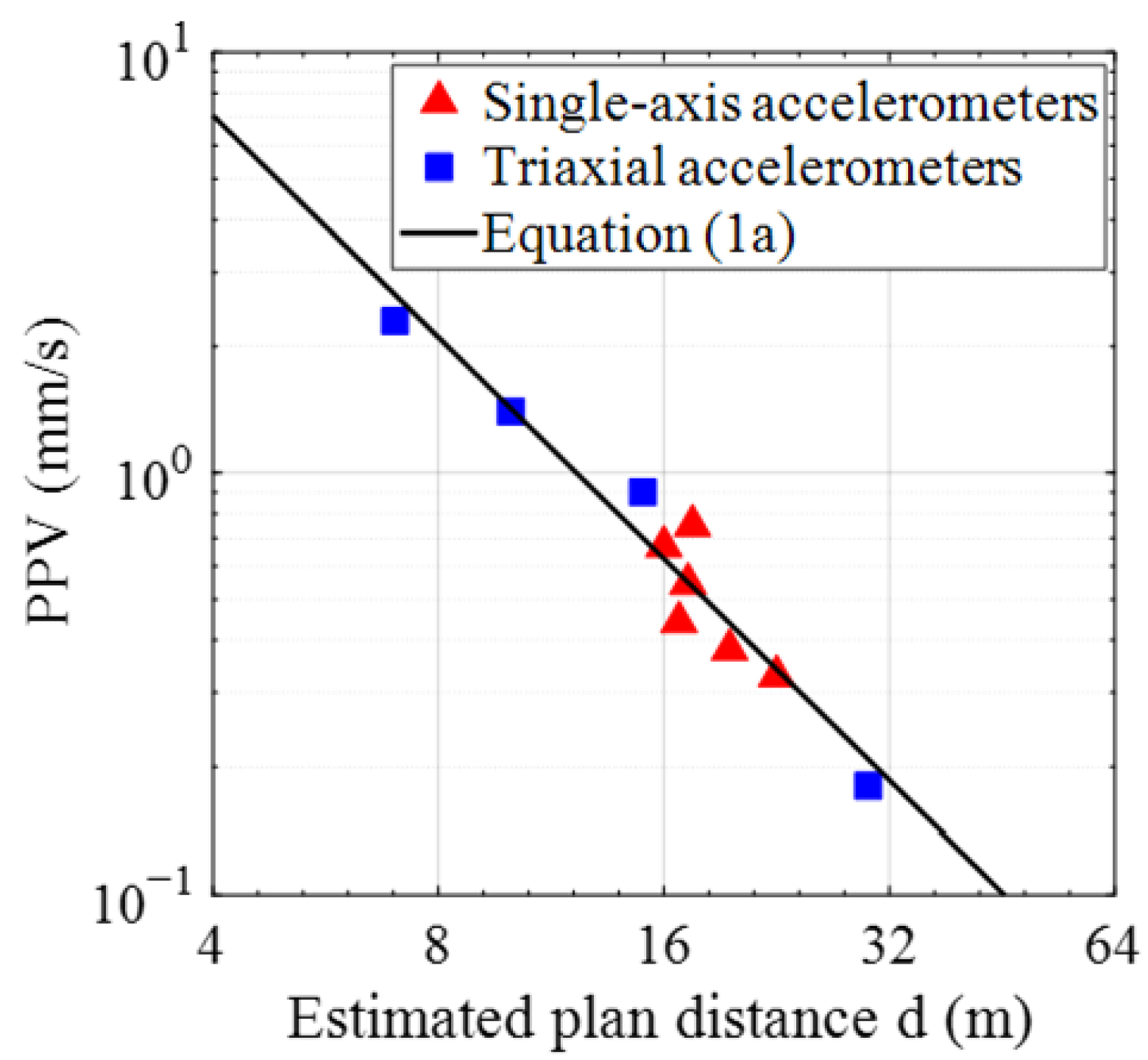
4.2. Global Vibration Intensity Prediction

Once the vibratory sheet pile driving work was localized, vibration intensities (e.g., PPV values) in the global area could be predicted. Figure 18 illustrates the PPV predictions based on the measured PPV values at various estimated distances from the localized vibratory driving location. It should be noted the estimated plan distances were used as the horizontal axis. The PPV values represent the vertical PPVs measured by six uniaxial accelerometers (in the vertical direction) and four triaxial accelerometers (the vertical component). A linear log–log best-fit line of Equation (1a) (n = 1.75, k = 80) was derived to estimate the vibration intensities of the entire field considering the site-specific nature of the tested construction site. The coefficient of determination (i.e., R squared) for the derived empirical relationship was calculated as 0.962 when using all measured data points.
Consequently, the vibration intensities in an extensive surrounding area rather than at a few monitoring points can be conveniently predicted using the derived empirical relationship and the estimated locations of the vibratory sheet pile driving work. In this way, the assessment of vibration impact is no longer limited to a few monitoring points, but rather extends to the entire surrounding environment.

5. Conclusions

In this study, we explored the global vibration impact assessment using several selected monitoring points on construction sites. By investigating the features of ground-borne vibration propagation due to vibratory pile driving work, we developed a time-based localization method to localize vibratory driving sources on construction sites. The localized vibratory driving sources and the site-specific empirical relationship derived from the field test data enable the estimation of vibration intensities over an extensive surrounding area rather than at a few monitoring points. The effects of pile toe depths, spatial relationships, and ground and construction conditions on localization performance were investigated through numerical parametric studies and field tests on a construction site with ongoing vibratory sheet pile driving work. The main findings are as follows:
  • For vibratory sheet pile driving at a certain depth, surface waves dominate the ground surface vibrations, while cylindrical shear waves from the pile shaft dominate the underground vibrations within the range of the pile shaft, and spherical body waves from the pile toe dominate underground vibrations at depths below the pile toe.
  • The time-based localization method assuming the single surface wave content along the ground surface is proved to be effective in localizing a vibratory driving source (e.g., vibratory sheet pile diving) on construction sites under different ground and construction conditions.
  • The layout of monitoring points has a notable effect on the localization performance. Both numerical simulations and field tests of vibratory sheet pile driving show that using a layout of monitoring points deployed in both directions surrounding the driving location can achieve a better localization performance.
  • The localized driving location and the estimated vibration attenuation formula can jointly estimate vibration intensity in the entire surrounding area rather than at a few monitored points, and then realize a global vibration impact assessment.
This study achieves an acceptable localization performance of unknown vibratory driving sources under the prerequisite that the ground is regarded as an infinite half-space domain with homogeneous soil properties. However, complex vibration propagations can be encountered due to soil stratification and geometric irregularity, which may result in the potential degradation of localization performance. Therefore, such complexity should be investigated in future studies.

Author Contributions

Data curation, methodology, software, investigation, validation, visualization, writing—original draft preparation, S.W.; conceptualization, supervision, funding acquisition, project administration, writing—review and editing, S.Z. All authors have read and agreed to the published version of the manuscript.

Funding

This research was funded by the National Key Research and Development Program of China (grant no. 2019YFB1600700) and the Hong Kong Polytechnic University (grant nos. ZE2L, BBWJ, ZVX6, ZJMV).

Institutional Review Board Statement

Not applicable.

Informed Consent Statement

Not applicable.

Data Availability Statement

The data generated or used during the study appear in the published article.

Acknowledgments

The authors would like to thank the editor and the reviewers for their contributions.

Conflicts of Interest

The authors declare no conflict of interest.

References

  1. BS ISO 4866; Mechanical Vibration and Shock, Vibration of Fixed Structures, Guidelines for the Measurement of Vibrations and Evaluation of Their Effects on Structures. BSI Group: London, UK, 2010.
  2. BS 5228-2; Code of Practice for Noise and Vibration Control on Construction and Open Sites, Part 2: Vibration. European Committee for Standardization: Brussels, Belgium, 2009.
  3. Jim, A.; David, B.; Harjodh, G.; Wesley, L. Transportation and Construction Vibration Guidance Manual; CT-HWANP-RT-13-069.25.3; California Department of Transportation Division of Environmental Analysis Environmental Engineering Hazardous Waste, Air, Noise, and Paleontology Office: Sacramento, CA, USA, 2013.
  4. DIN 4150-3; Structural vibration—Part 3: Effects of Vibration on Structures. German Institute for Standardisation: Berlin, Germany, 1999.
  5. Deckner, F.; Viking, K.; Hintze, S. Ground vibrations due to pile and sheet pile driving: Prediction models of today. In Proceedings of the 22nd European Young Geotechnical Engineers Conference, Gothenburg, Sweden, 26–29 August 2012; pp. 107–112. [Google Scholar]
  6. Richart, F.E.; Hall, J.R.; Woods, R.D. Vibrations of Soils and Foundations; Prentice Hall: Englewood Cliffs, NJ, USA, 1970; pp. 60–92. [Google Scholar]
  7. Wiss, J.F. Construction vibrations: State-of-the-art. J. Geotech. Eng. Div. 1981, 107, 167–181. [Google Scholar] [CrossRef]
  8. Attewell, P.B.; Selby, A.R.; O’Donnell, L. Estimation of ground vibration from driven piling based on statistical analyses of recorded data. Geotech. Geol. Eng. 1992, 10, 41–59. [Google Scholar] [CrossRef]
  9. Ramshaw, C.L.; Selby, A.R.; Bettess, P. Computer Ground Waves Due to Piling. In Proceedings of the Geotechnical Earthquake Engineering and Soil Dynamics III, Seattle, WA, USA, 3–6 August 1998; pp. 1484–1495. [Google Scholar]
  10. Masoumi, H.R.; François, S.; Degrande, G. A non-linear coupled finite element-boundary element model for the prediction of vibrations due to vibratory and impact pile driving. Int. J. Numer. Anal. Methods Geomech. 2009, 33, 245–274. [Google Scholar] [CrossRef]
  11. Khoubani, A.; Ahmadi, M.M. Numerical study of ground vibration due to impact pile driving. Proc. Inst. Civ. Eng. Geotech. Eng. 2014, 167, 28–39. [Google Scholar] [CrossRef]
  12. Rooz, A.F.H.; Hamidi, A. Numerical analysis of factors affecting ground vibrations due to continuous impact pile driving. Int. J. Geomech. 2017, 17, 04017107. [Google Scholar] [CrossRef]
  13. Jongmans, D. Prediction of ground vibrations caused by pile driving: A new methodology. Eng. Geol. 1996, 42, 25–36. [Google Scholar] [CrossRef]
  14. Svinkin, M.R. Predicting soil and structure vibrations from impact machines. J. Geotech. Geoenviron. Eng. 2002, 128, 602–612. [Google Scholar] [CrossRef]
  15. Athanasopoulos, G.A.; Pelekis, P.C. Ground vibrations from sheetpile driving in urban environment: Measurement, analysis and effects on buildings and occupants. Soil Dyn. Earthq. Eng. 2000, 19, 371–387. [Google Scholar] [CrossRef]
  16. Zhu, S.; Shi, X.; Leung, R.C.; Cheng, L.; Ng, S.; Zhang, X.; Wang, Y. Impact of construction-induced vibration on vibration-sensitive medical equipment: A case study. Adv. Struct. Eng. 2014, 17, 907–920. [Google Scholar] [CrossRef]
  17. Dowding, C.H. Construction Vibrations; Prentice Hall: Englewood Cliffs, NJ, USA, 1996; pp. 425–453. [Google Scholar]
  18. Svinkin, M.R. Minimizing construction vibration effects. Pract. Period. Struct. Des. Constr. 2004, 9, 108–115. [Google Scholar] [CrossRef]
  19. Manvell, D. Noise and vibration monitoring around construction sites-examples of standards and practice from around the world. In Proceedings of the INTER-NOISE and NOISE-CON Congress and Conference Proceedings, Hong Kong, China, 27–30 August 2017; Institute of Noise Control Engineering: Washington, DC, USA, 2017; Volume 255, pp. 5046–5054. [Google Scholar]
  20. Zhang, M.; Tao, M.; Gautreau, G.; Zhang, Z.D. Statistical approach to determining ground vibration monitoring distance during pile driving. Pract. Period. Struct. Des. Constr. 2013, 18, 196–204. [Google Scholar] [CrossRef]
  21. Lemke, J. Remote vibration monitoring system using wireless internet data transfer. In Proceedings of the SPIE’s 5th Annual International Symposium on Nondestructive Evaluation and Health Monitoring of Aging Infrastructure, Newport Beach, CA, USA, 9 June 2000; pp. 436–445. [Google Scholar] [CrossRef]
  22. Veggeberg, K. Wireless Noise and Vibration Management System for Construction Sites. Struct. Dyn. 2011, 3, 1553–1557. [Google Scholar] [CrossRef]
  23. Meng, Q.; Zhu, S. Developing IoT sensing system for construction-induced vibration monitoring and impact assessment. Sensors 2020, 20, 6120. [Google Scholar] [CrossRef] [PubMed]
  24. Wang, S.; Zhu, S. Impact source localization and vibration intensity prediction on construction sites. Measurement 2021, 175, 109148. [Google Scholar] [CrossRef]
  25. Zerwer, A.; Cascante, G.; Hutchinson, J. Parameter estimation in finite element simulations of Rayleigh waves. J. Geotech. Geoenviron. Eng. 2002, 128, 250–261. [Google Scholar] [CrossRef]
  26. Hibbitt, D.; Karlsson, B.; Sorensen, P. Abaqus User’s Manual, version 6.13; Hibbitt, Karlsson and Sorensen Inc.: Providence, RI, USA, 2013. [Google Scholar]
  27. BS EN 10248; Hot Rolled Sheet Piling of Non-Alloy Steels. Technical Delivery Conditions. BSI Group: London, UK, 1996.
  28. Novotny, J.W.; Perkins, W.W.; Price, J.N.; Watts, R.L.; Wheeler, H.C. NAVFAC (CHESDIV) (Naval Facilities Engineering Command) (Chesapeake Division) Standards and Criteria Program, Phase 1A, Volume 1; Naval Undersea Center: San Diego, CA, USA, 1975.
  29. Woods, R.D. Dynamic Effects of Pile Installations on Adjacent Structures; National Academy Press: Washington, DC, USA, 1997; pp. 11–15. [Google Scholar]
  30. Kim, D.S.; Lee, J.S. Propagation and attenuation characteristics of various ground vibrations. Soil Dyn. Earthq. Eng. 2000, 19, 115–126. [Google Scholar] [CrossRef]
  31. Branch, M.A.; Grace, A. Matlab Optimization Toolbox; The Mathworks Inc.: Natick, MA, USA, 1996. [Google Scholar]
  32. Deckner, F.; Viking, K.; Hintze, S. Wave patterns in the ground: Case studies related to vibratory sheet pile driving. Geotech. Geol. Eng. 2017, 35, 2863–2878. [Google Scholar] [CrossRef] [Green Version]
Figure 1. Numerical modeling of vibratory sheet pile driving. (a) Isometric view of the full model; (b) top view of the full model; (c) sheet pile pre-inserted at any target depth.
Applsci 12 01946 g001
Figure 2. Wave propagation snapshots at different time steps during vibratory sheet pile driving when pre-embedding the pile toe 10 m below the ground surface. (a) 50ms; (b) 300 ms; (c) 550 ms; (d) 700 ms.
Applsci 12 01946 g002
Figure 3. Definitions of plan distance d (m) and radial distance r (m).
Applsci 12 01946 g003
Figure 4. Computed vertical velocity time histories of the pile and three soil nodes at different depths (Z = 0, −7 m, −25 m) and one plan distance (d = 20 m) when pile toe is pre-embedded at 10 m below the ground surface.
Applsci 12 01946 g004
Figure 5. Distances vs. ToAs when pile toe is pre-embedded 10 m below the ground surface. (a) d vs. ToA of ground surface points on X-Y plane (Z = 0); (b) d vs. ToA of buried points on X-Z plane (−10 m < Z < −3 m); (c) r vs. ToA of buried points on X-Z plane (−30 m < Z < −10 m).
Applsci 12 01946 g005
Figure 6. Particle motions of soil nodes at different plan distances and depths when pile toe is pre-embedded 10 m below the ground surface.
Applsci 12 01946 g006
Figure 7. Two layouts of monitoring points deployed on the ground surface. (a) Linear layout; (b) square layout.
Applsci 12 01946 g007
Figure 8. Localization of horizontal coordinates when pile toe is placed on the ground surface. (Note: MP—monitoring points, AVDL—actual vibratory driving location, EVDL—estimated vibratory driving location).
Applsci 12 01946 g008
Figure 9. Localization of horizontal coordinates when pile toe is pre-embedded 10 m below the ground surface. (a) Linear layout; (b) square layout. (Note: MP—monitoring points, AVDL—actual vibratory driving location, EVDL—estimated vibratory driving location).
Applsci 12 01946 g009
Figure 10. Localization of horizontal coordinates when pile driving takes place in different ground conditions. (a) vs = 60 m/s; (b) vs = 250 m/s. (Note: MP—monitoring points, AVDL—actual vibratory driving location, EVDL—estimated vibratory driving location).
Applsci 12 01946 g010
Figure 11. Localization of horizontal coordinates when pile driving force operates at different frequencies. (a) f0 = 40 Hz; (b) f0 = 60 Hz. (Note: MP—monitoring points, AVDL—actual vibratory driving location, EVDL—estimated vibratory driving location).
Applsci 12 01946 g011
Figure 12. Localization of horizontal coordinates when the pile–soil interface is defined with different pile–soil friction coefficients. (a) μ = 0.1; (b) μ = 0.4. (Note: MP—monitoring points, AVDL—actual vibratory driving location, EVDL—estimated vibratory driving location).
Applsci 12 01946 g012
Figure 13. Photos of field validation test setup. (a) The construction site; (b) the vibratory sheet pile driving work in progress; (c) the first set of data acquisition systems integrated with (d) the single-axis accelerometers; (e) the second set of data acquisition system integrated with (f) the triaxial accelerometer.
Applsci 12 01946 g013
Figure 14. The layout of monitoring points.
Applsci 12 01946 g014
Figure 15. Particle vibration paths at one plan distance (d = 15 m) by one triaxial accelerometer.
Applsci 12 01946 g015
Figure 16. Vertical vibration signals recorded at the six monitoring points (P1–P6) by single-axis accelerometers.
Applsci 12 01946 g016
Figure 17. Localization results using monitoring points in (a) a linear layout; (b) a right-angle layout.
Applsci 12 01946 g017
Figure 18. PPV (mm/s) predictions based on measured vibration intensities at estimated plan distances d (m) from the localized vibratory driving source.
Applsci 12 01946 g018
Table 1. Properties of the simulated sheet pile.
Pile TypeU-Type Dimensions
b (m)–h (m)–t (m)
Length (m)Mass (kg/m)
Steel sheet0.4–0.17–0.0161576.1
Table 2. Soil properties reported in the previous studies [10,11,12].
Soil TypeDensity (kg/m3)Modulus of Elasticity (MPa)Poisson’s RatioFriction Angle (Degrees)Cohesion (kPa)
Sandy clay2000800.42515
Table 3. Relative errors of the estimated coordinates.
Actual Vibratory Sheet Pile Driving LocationsPile Toe on the Ground SurfacePile Toe 10 m below the Ground Surface
Linear LayoutLinear LayoutSquare Layout
X (%)Y (%)X (%)Y (%)X (%)Y (%)
S11.850.022.670.021.000.02
S21.700.023.330.020.670.02
S32.000.023.000.021.750.02
S40.920.081.750.120.920.10
S51.670.023.330.021.330.02
S61.380.082.220.081.380.14
S71.500.172.250.191.420.15
S81.500.084.000.091.500.09
S92.080.191.670.191.580.17
Mean1.620.082.690.081.280.08
Max.2.080.194.000.191.750.17
Table 4. Mean and maximum relative errors of the estimated coordinates from sensitivity studies.
Investigated ParametersMeanMax.
X (%)Y (%)X (%)Y (%)
Shear wave velocity
(when f0 = 20 Hz,
μ = 0.25)
vs = 60 m/s2.520.084.170.25
vs = 120 m/s2.690.084.000.19
vs = 250 m/s3.560.074.780.25
Vibratory driving frequency
(when vs = 120 m/s,
μ = 0.25)
f0 = 20 Hz2.690.084.000.19
f0 = 40 Hz2.710.063.680.17
f0 = 60 Hz3.730.075.300.21
Pile–soil friction coefficient
(when vs = 120 m/s,
f0 = 20 Hz)
μ = 0.13.350.095.070.17
μ = 0.252.690.084.000.19
μ = 0.41.750.073.080.25
Publisher’s Note: MDPI stays neutral with regard to jurisdictional claims in published maps and institutional affiliations.

