A Bus Passenger Flow Prediction Model Fused with Point-of-Interest Data Based on Extreme Gradient Boosting

Abstract

Bus operation scheduling is closely related to passenger flow. Accurate bus passenger flow prediction can help improve urban bus planning and service quality and reduce the cost of bus operation. Using machine learning algorithms to find the rules of urban bus passenger flow has become one of the research hotspots in the field of public transportation, especially with the rise of big data technology. Bus IC card data are an important data resource and are more valuable to passenger flow prediction in comparison with manual survey data. Aiming at the balance between efficiency and accuracy of passenger flow prediction for multiple lines, we propose a novel passenger flow prediction model based on the point-of-interest (POI) data and extreme gradient boosting (XGBoost), called PFP-XPOI. Firstly, we collected POI data around bus stops based on the Amap Web service application interface. Secondly, three dimensions were considered for building the model. Finally, the XGBoost algorithm was chosen to train the model for each bus line. Results show that the model has higher prediction accuracy through comparison with other models, and thus this method can be used for short-term passenger flow forecasting using bus IC cards. It plays a very important role in providing decision basis for more refined bus operation management.

1. Introduction

Bus transport is a critical component of the transportation system. With the significant progress of urbanization, buses are becoming the leading force in public transportation. For example, Beijing has one of the most crowded bus networks at present. According to the statistics of Beijing Public Transport Corporation, in 2020, there were 1207 bus lines (including suburban lines) with a total length of 28,400 km. The volume of the average daily passenger in Beijing has far exceeded a person-time of 5 million, and the total annual passenger volume has reached a person-time of 1.9 billion [1]. Passengers’ behavior can be understood by analyzing smart card data [2]. The large quantity of data collected by smart cards offers more detailed characteristics in the time and space dimension than any other types of data. To improve the bus service quality, an accurate and proactive passenger flow prediction approach is necessary [3,4]. Availability of smart card data has offered more opportunities for the prediction work [5]. The prediction results can help the bus operators optimize resource scheduling and save operating costs as well as assist passengers in making better decisions by adjusting their travel paths and departure time. Furthermore, this approach is useful for the government to assess risk and guarantee public safety.

There are two main fields of study in passenger flow prediction, namely time series models and machine learning methods. Most time series models are designed based on the autoregressive integrated moving average model (ARIMA) [6,7,8]. However, time series models only predict different states for a single target, such as the number of passengers at a specific bus stop at different times. When predicting multiple targets for the whole traffic network, this kind of method maintains various models for different objects. As for the machine learning methods, they convert the time series into a supervised learning problem, solved by machine learning algorithms [9].

Passengers’ chief travel destinations are closely related to daily work and life, such as work areas, residential quarters, markets and tourist attractions. The smart card data can be applied to analyze the passenger flow characteristics between different POI locations. From the above point of view, a PFP-XPOI model was investigated in this study for the prediction of bus passenger flow. The main contributions of this study are as follows:

• A novel bus passenger flow prediction model is proposed. The model takes the predicting accuracy and the predicting efficiency into account. The model improves the dimensionality of bus IC card data by fusing POI, so that large-scale low-dimensional data have more feature representation, which ensures the accuracy of prediction. The XGBoost algorithm has the advantage of fast operation, contributing to reducing the total training time of the passenger flow prediction model for multiple lines to achieve the goal of efficient training.
• Extensive experiments were conducted on historical passenger flow datasets of Beijing. After preprocessing the original data and matching the POI data, the XGBoost algorithm can be used to build a unified prediction model for different stations of the bus line, which can effectively improve the training efficiency of the model. In addition, comparison with the existing methods verifies the practicability and effectiveness of the proposed model.

In the following, Section 2 reviews literature on bus passenger flow prediction methods. Section 3 elaborates the proposed method in detail, covering data processing and modeling. The prediction results and relevant discussion are given in Section 4. Finally, Section 5 concludes this paper.

2. Related Work

Bus passenger flow prediction has been a popular research topic in recent years. Generally, approaches to this topic can be divided into parametric and non-parametric methods.

In parametric methods, the ARIMA model has been applied successfully [10]. A pioneering paper [11] introduced ARIMA into traffic prediction. Later, many variants of ARIMA were proposed by combining modes in passenger flow, especially in terms of time. Different seasonal autoregressive integrated moving average (SARIMA) models were tested, and the appropriate one was chosen to generate rail passenger traffic forecasts in [6]. The SARIMA time series model was chosen to forecast the airport terminal passenger flow in [7]. Other methods were further combined with ARIMA by some researchers. A hybrid model combining symbolic regression and ARIMA was proposed to enhance the forecasting accuracy [12]. Fused with a Kalman filter, the framework consisting of three sequential stages was designed to predict the passenger flow at bus stops [13]. These methods assumed that the data change only over time, so they relied heavily on the similarity of time-varying patterns between historical data and future forecast data, ignoring the role of external influences. It would be complex for these approaches to train a specific passenger flow forecasting model for every station in a certain line.

Non-parametric models, represented by machine learning methods, were also utilized for predicting traffic characteristics. Machine learning methods have been gaining popularity due to their outstanding performance in mining the underlying patterns in traffic dynamics. The support vector machine (SVM)-based approach can map low-dimensional data to a high-dimensional space with kernel functions. The complexity of the computation depends on the number of support vectors rather than the dimensionality of the sample space, which avoids the “dimensionality disaster”. Hybrid models connecting the classical ARIMA and SVM were built in [14], which performed better than the use of a single model. A model combining the advantages of Wavelet and SVM was presented to predict different kinds of passenger flows in the subway system in [15]. These SVM-based methods had satisfying passenger flow forecasting performance. A well-known machine learning paper [16] showed that machine learning methods dominate in terms of both accuracy and forecasting horizons.

Methods based on deep learning were also applied to passenger flow prediction. Liu et al. proposed a deep learning-based architecture integrating the domain knowledge in transportation modeling to explore short-term metro passenger flow prediction. [17]. The real-time information was taken into consideration in passenger flow prediction based on the LSTM [18]. An improved spatiotemporal long short-term memory model (Sp-LSTM) based on deep learning techniques and big data was developed to forecast short-term outbound passenger volume at urban rail stations in [19]. The XGBoost algorithm is one of the core algorithms in data science and machine learning. XGBoost is an improved CART algorithm. The results of the XGBoost algorithm in a Kaggle machine learning competition were introduced in [20]. Nielsen explained why XGBoost wins every machine learning competition in his master’s thesis [21]. Dong et al. predicted short-term traffic flow using XGBoost and compared its accuracy with that of SVM [22]. Lee et al. trained XGBoost to model express train preference using smart card and train log data and achieved notable accuracy [23].

Mass data are an important condition for the algorithm to function. The availability of big data sources such as smart card data and POI provide a perfect chance to produce new insights into transport demand modeling [24]. Smart card records, the transactions of passengers in the public transit network, are a valuable source of urban mobility data [25]. In order to ensure the prediction accuracy, it is vital to increase the dimensions of bus smart card data. By introducing POI data to characterize the attributes of certain areas, the model could be more fully trained to improve accuracy [26]. Accordingly, combining the POI and smart card data has the potential to reveal trip purposes of passengers.

To balance the efficiency and accuracy of prediction, we propose a novel passenger flow prediction model based on extreme gradient boosting (XGBoost) and the point-of-interest (POI) data, referred to as PFP-XPOI.

3. Methodology

3.1. IC Card Data Processing and POI Description

The target data for this study were the number of passengers boarding and alighting at each bus station of the two selected routes during the morning peak hours (7:00–9:00, with a half-hour interval containing four time periods). The two selected bus routes are line 56008 and line 685. The bus route 56008 is a bus loop that passes through the central business district (CBD) and has a very large passenger flow, while the bus route 685 has a relatively small passenger flow, and the two routes interchange at Fangzhuangqiaoxi bus station. The PFP-XPOI model training set is from 8 October 2015 to 25 October 2015, and the test set is from 26 October 2015 to 30 October 2015. The total size of the dataset is 50 GB, containing 150 million swipe records. After being clustered by station and time period, the total number of data is 3 million.

The process of cleaning the IC card data is to remove the data with empty boarding or alighting time, and to delete the data with an interval of more than 3 h from boarding to alighting time. The cleaned data account for about 1% of the total data.

POI is a term in GIS which refers to all geographical objects that can be abstracted as points, especially some geographical entities that are closely related to people’s life, such as schools, banks, restaurants, gas stations, hospitals and supermarkets. The main use of POI is to describe the address of things or events, and the number of different types of POI in a region can characterize the attributes of the region. In this study, POI data collection around bus stops was carried out based on the Amap application programming interface (API). The API refers to a series of functions that have been predefined. Developers can implement existing functions by calling API functions without accessing the source code or understanding the details of internal working mechanisms. The Amap location based services (LBS) open platform provides professional electronic maps and location services to the public. When developers integrate the corresponding software development kit (SDK), the interface can be invoked to implement many functions, such as map display, label POI, location retrieval, data storage and analysis.

The collection process is divided into four parts: acquiring global positioning system (GPS) latitude and longitude of each station based on bus operation data, converting GPS latitude and longitude into Amap coordinates, collecting POI information based on Amap coordinates and organizing POI data into corresponding fields. To convert GPS coordinates to Amap coordinates, we need to apply the coordinate conversion method and add the corresponding parameters to the URL of the GET request. The main parameters for applying this method are listed in

Table 1. Coordinate conversion and peripheral searching parameters using Amap API.

Parameter	Meaning
key	Users apply for API types on the official website of AMap.
location	Longitude and latitude are divided by “,”. Longitude is the former and latitude is the latter. The decimal point of latitude and longitude should not exceed 6 digits.
coordsys	The original coordinate system.
types	POI types. The classification code consists of six digits. The first two numbers represent large categories, the middle two represent medium categories and the last two represent small categories.
city	City of inquiry.
radius	Radius of the inquiry. The value range is from 0 to 50,000.
Output	Return to data format type.

.

3.2. Passenger Flow Prediction Model

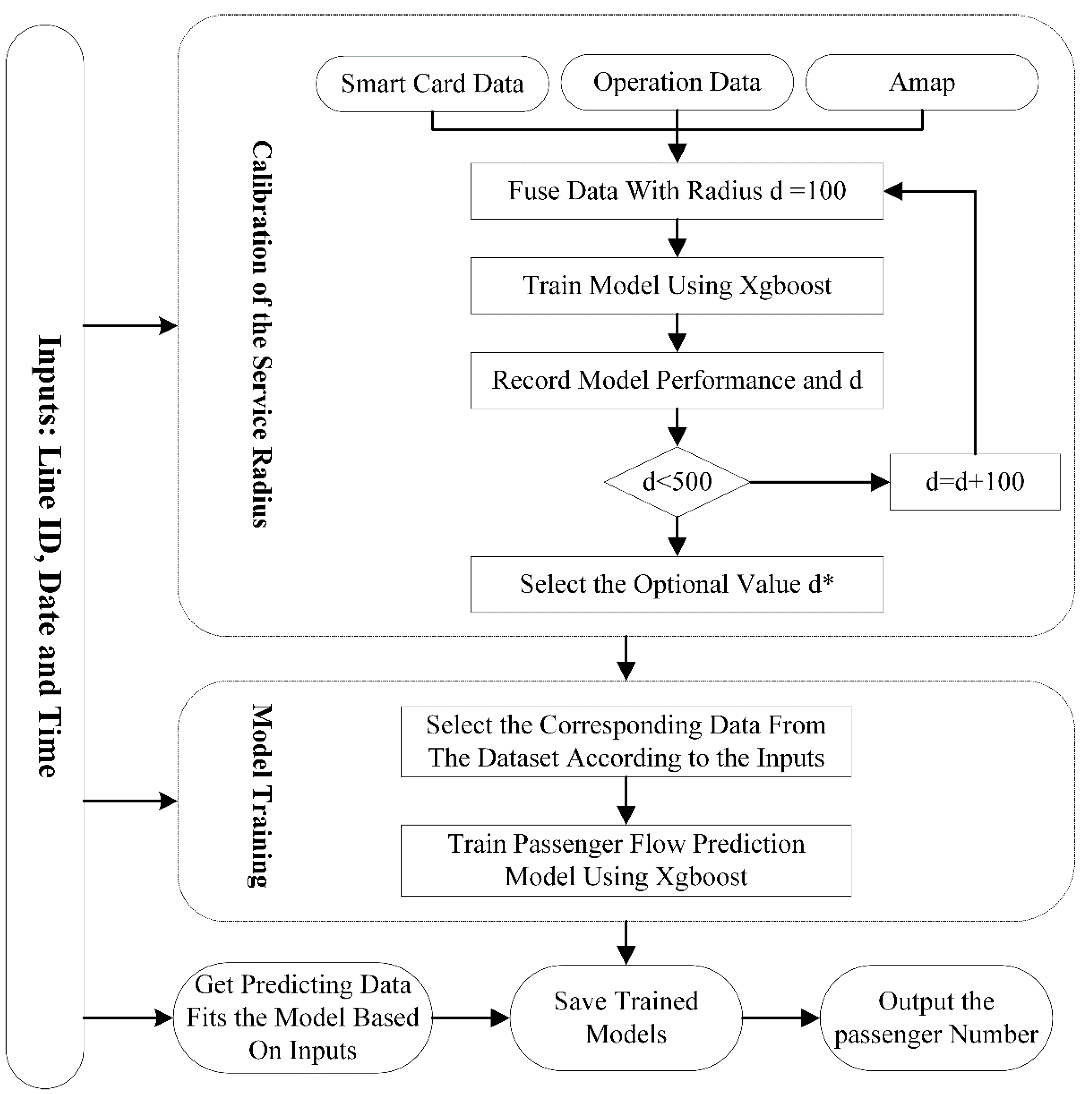
We propose the PFP-XPOI model for passenger flow prediction. The features selected for this model comprise the following three dimensions. One dimension is the information related to the line and the station, such as the line code of the station and the latitude and longitude of the station. Another dimension is the time period and the date when the IC card data are generated. The third dimension is the number of different types of POI around the station, including the number of companies and research institutions, etc.

This model consists of two parts. One part is the calibration of the service radius between the bus station and POI data, and the other part is the training of the passenger flow prediction model for each line. We built the PFP-XPOI model based on the following steps. The dataset $D_S$ is a sample space, and we can represent the machine learning model as

$$M\left(x\in D_S\right)\to y.$$

(1)

where $M$ means a mapping from data point $x$ to its true value $y$. After taking POI into account, we can add a new dataset to the original one. Namely

$$D_n=f_{dis}\left(D_S,D_P\right).$$

(2)

where $D_n$ is the updated sample space. $D_P$ means the POI data set. $f_{dis}$ refers to a distance-based function between bus stations and POI. In this model, distances were set to 100, 200, 300, 400 and 500 m, forming 5 datasets. After that, to obtain the optimal service radius d*, the machine learning model for different datasets was trained. Finally, d* can help us find the best dataset. We trained a passenger flow prediction model for each line based on this dataset using XGBoost. The detail of the PFP-XPOI model is shown in Figure 1.

3.3. Model Training

In this research, XGBoost was used to train the model for every bus line. XGBoost is scalable in a wide range of situations because of the optimization of some important algorithms and systems, including a novel tree learning algorithm for handling sparse data and a rational weighted quantile sketch process for controlling instance weights in approximate tree learning. Its operating time is 10 times faster than other popular programs on a single device, and it scales up to billions of examples in the case of distributed or limited memory. Parallel and distributed computing makes learning faster which enables quicker model exploration. In addition, utilization of out-of-core calculation enables hundred millions of examples to be processed on a desktop. These techniques can be connected to create an end-to-end system that extends to big data with the fewest cluster resources.

XGBoost is one kind of boosting tree model aiming to generate certain tree models for prediction. The tree ensemble model includes independent variable $x_i$ and dependent variable $y_i$ and estimates the target value ${\overline{y}}_i$ using T additive functions. The function can be expressed as

$${\overline{y}}_i=\varphi \left(x_i\right)={{\displaystyle \sum }}_{t=1}^T{f}_t\left(x_i\right)$$

(3)

where ${\overline{y}}_i$ is the target value; $y_i$ is the dependent variable ($y_i$ is 1 if the passenger boards on or alights from the bus; otherwise, it is 0); $x_i$ is the independent variable; t is the features; $f_t\left(x_i\right)$ is the model at the tth iteration and T is the number of tree functions.

The objective is to minimize the loss function $L^{\left(t\right)}$ at the tth iteration which can be expressed as

$$L^{\left(t\right)}={{\displaystyle \sum }}_{i=1}^{n}l\left(y_i,{\overline{y}}_i^{\left(t-1\right)}+f_t\left(x_i\right)\right)+\mathsf{\Omega }\left(f_t\right)$$

(4)

where $l$ represents the loss function and ${\overline{y}}_i^{\left(t-1\right)}$ means the predicted value of the (t − 1)th iteration. The additional term $\mathsf{\Omega }\left(f_t\right)$ plays a role in reducing the complexity of the model.

Approximating $L^{\left(t\right)}$ with a second-order Taylor expansion for $l\left(y_i, {\overline{y}}_i^{\left(t-1\right)}+f_t\left(x_i\right)\right)$ at ${\overline{y}}_i^{\left(t-1\right)}$, the Equation (4) becomes

$$L^{\left(t\right)}\simeq {{\displaystyle \sum }}_{i=1}^n\left[l\left(y_i,{\overline{y}}_i^{\left(t-1\right)}\right)+g_i{f}_t\left(x_i\right)+\frac{1}{2}{h}_i{f}_t^2\left(x_i\right)\right]+\mathsf{\Omega }\left(f_t\right)$$

(5)

where $g_i=\frac{\partial l\left(y_i,{\overline{y}}_i^{\left(t-1\right)}\right)}{\partial {\overline{y}}_i^{\left(t-1\right)}}$, $h_i=\frac{{\partial }^{2}l\left(y_i,{\overline{y}}_i^{\left(t-1\right)}\right)}{\partial {\overline{y}}_i^{\left(t-1\right)}}$.

$l\left(y_i,{\overline{y}}_i^{\left(t-1\right)}\right)$ in Equation (5) can be disregarded as it is a constant term. Therefore, we obtain a new simplified objective function as follows.

$$L^{\left(t\right)}={{\displaystyle \sum }}_{i=1}^n\left[g_i{f}_t\left(x_i\right)+\frac{1}{2}{h}_i{f}_t^2\left(x_i\right)\right]+\mathsf{\Omega }\left(f_t\right)$$

(6)

For a tree structure, the samples can be grouped according to the leaf node, and the samples that fall into the same leaf node can be represented as $I_j=\left\{i\right|x_i\in j\}$. j is the leaf node number. By introducing $w_j$ as the score of leaf j, we can rewrite Equation (6) as follows.

$$\begin{array}{c}{L}^{\left(t\right)}={{\displaystyle \sum }}_{i=1}^n\left[g_i{f}_t\left(x_i\right)+\frac{1}{2}{h}_i{f}_t^2\left(x_i\right)\right]+\gamma T+\frac{1}{2}\lambda {{\displaystyle \sum }}_{j=1}^T{w}_j^2\\ ={{\displaystyle \sum }}_{j=1}^{T}l{\displaystyle {\displaystyle \sum }_{j=1}^T}\left[\left({\displaystyle \sum }_{i\in I_j}{g}_i\right)w_j+\frac{1}{2}\left({\displaystyle \sum }_{i\in I_j}{h}_i+\lambda \right)w_j^2\right]+\gamma T\end{array}$$

(7)

where $\gamma$ controls the number of leaf nodes and $\lambda$ prevents overfitting.

Let the value of the first-order partial derivative function of y concerning x be equal to 0, and then the optimal weight $w_j^{*}$ of leaf $j$ can be calculated as

$$w_j^{*}=-\frac{G_i}{H_i+\lambda }$$

(8)

$L^{\left(t\right)}$ can finally be shown in Equation (9).

$$L^{\left(t\right)}=-\frac{1}{2}{{\displaystyle \sum }}_{j=1}^T\frac{G_i}{H_i+\lambda }+\gamma T$$

(9)

Normally it is impossible to enumerate all the possible tree structures. A greedy algorithm that starts from a single leaf and iteratively adds branches to the tree is used instead. Assume that $I_L$ and $I_R$ are the instance sets of left and right nodes after the split. Let $I=I_L{\displaystyle \cup }{I}_R$, and then the loss reduction after the split is given by

$$L_{spilt}=\frac{1}{2}\left(\frac{G_L}{H_L+\lambda }+\frac{G_R}{H_R+\lambda }-\frac{G}{H+\lambda }\right)-\gamma .$$

(10)

With the help of the process above, we can calculate a tree for prediction.

4. Results and Discussion

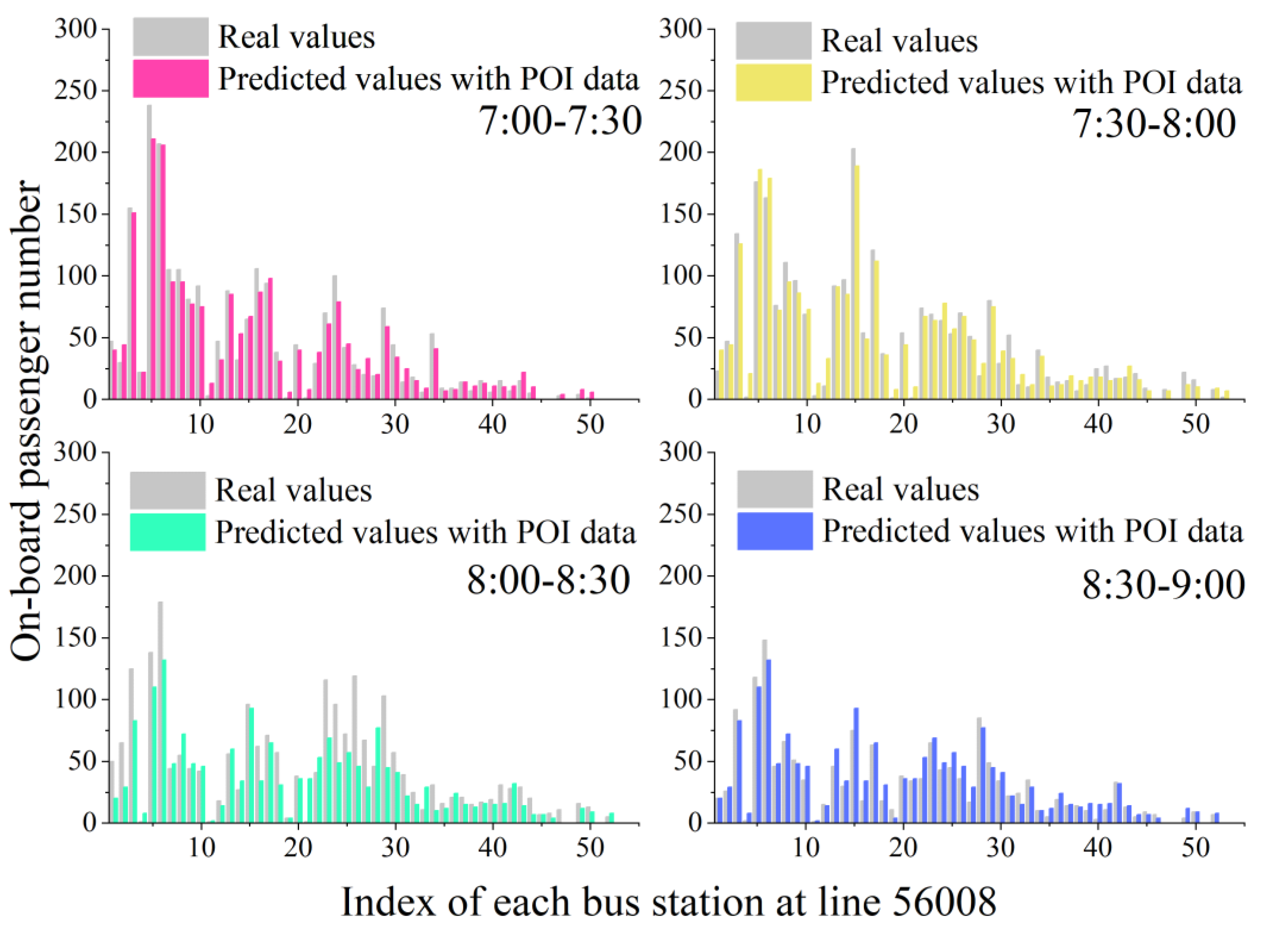
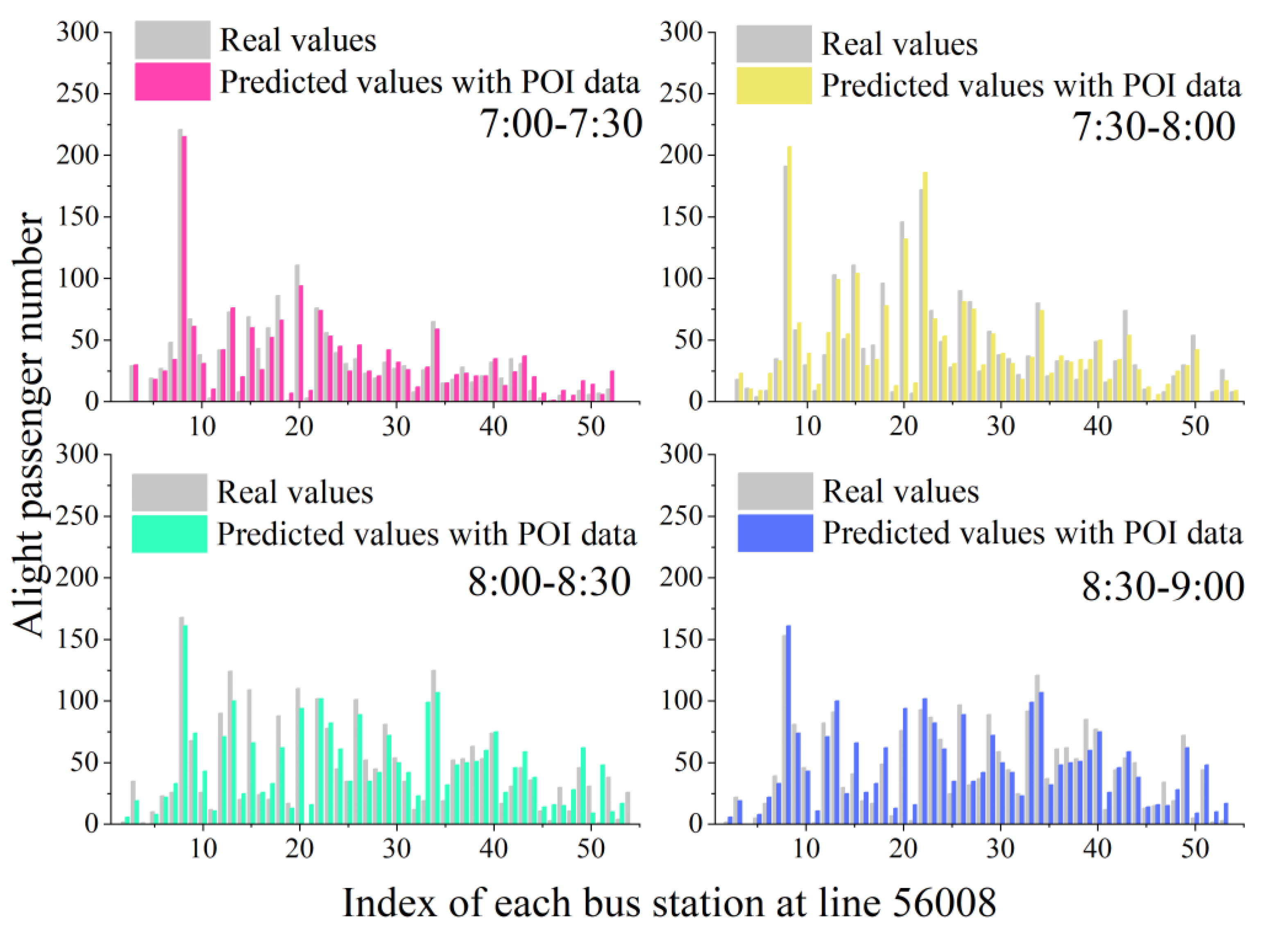
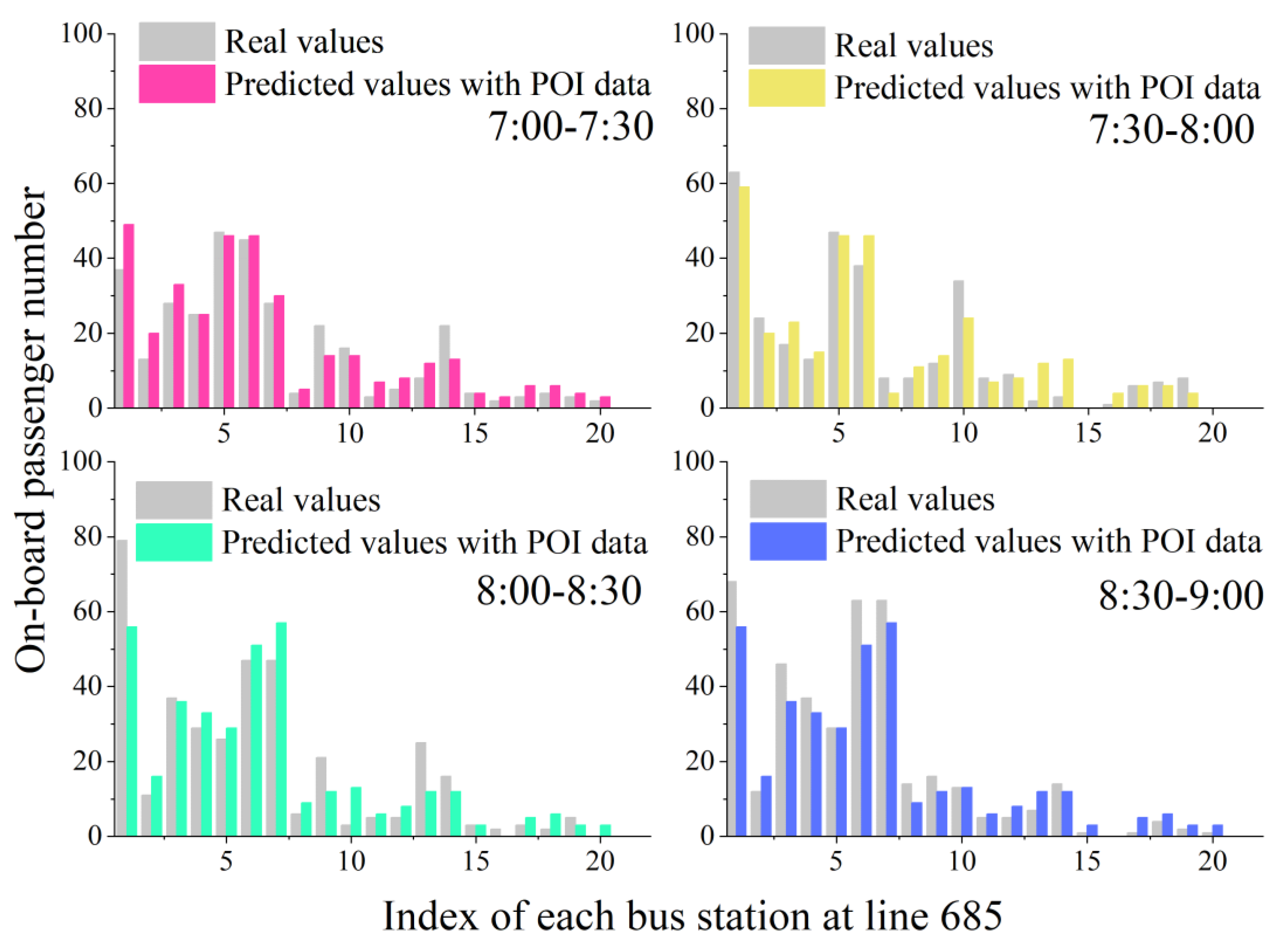
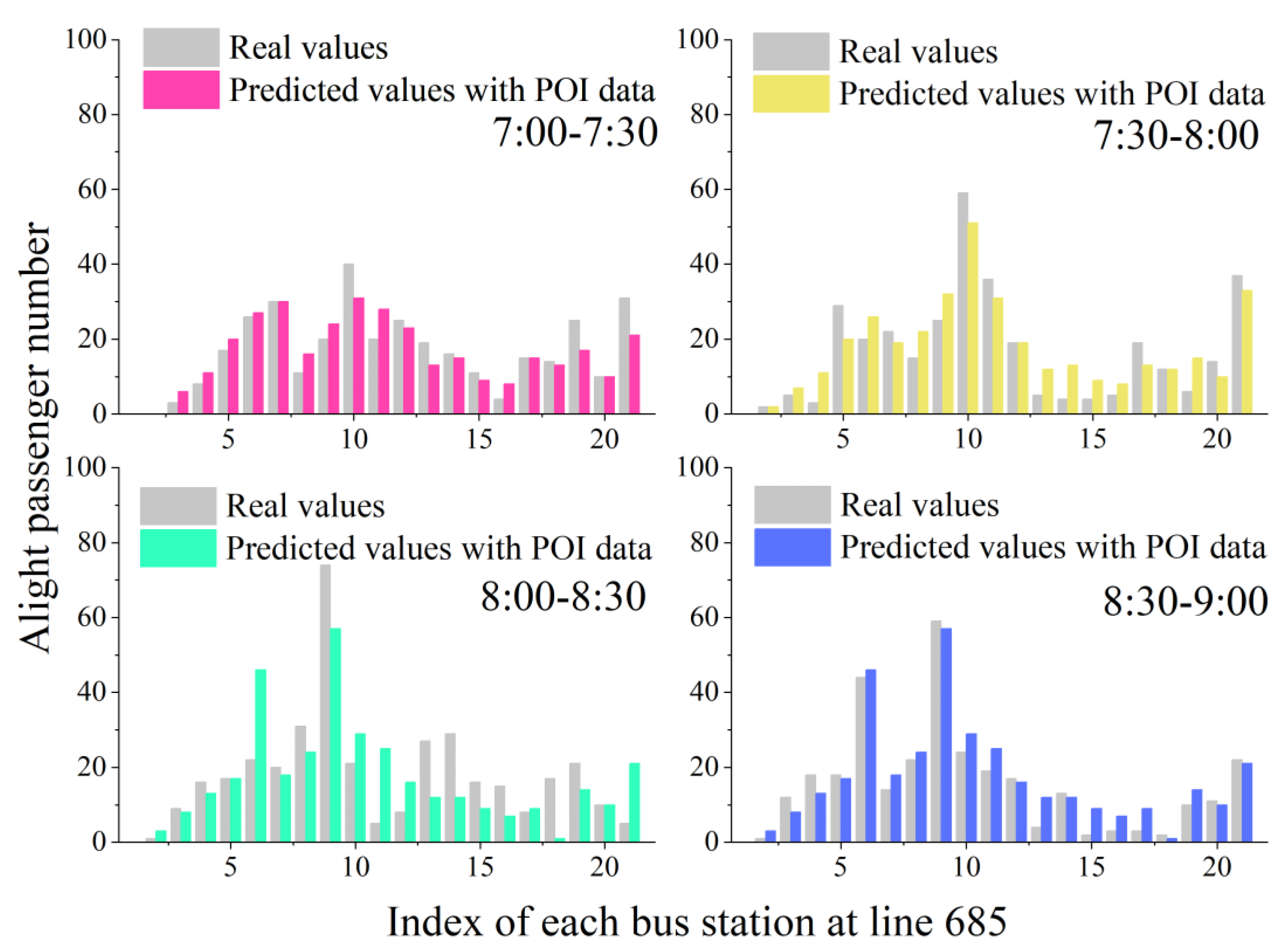
4.1. Peak Period Experiments

The training dataset used was extracted from 8 October 2015 to 25 October 2015. The test dataset is from 26 October 2015 to 30 October 2015. The two lines are 685 and 56008. Line 56008 has a large passenger volume because it is a major bus line on the third ring road in Beijing. Line 685 is a normal line that has a relatively small passenger volume. If the passenger numbers of the two lines are very large, the departure frequency will be relatively high; thus, we do not need to consider the transfer situation. If the passenger numbers of both lines are small, the number of passengers who need to transfer between lines will be much smaller, so there is little need to consider the transfer coordination. Therefore, after calculation, we chose these two lines as our experimental lines. These two lines can be transferred at Fangzhuangqiaoxi bus station.

With a Windows 10 operating system, a I7-8700k processor, and 32 GB memory, the PFP-XPOI model takes 20 min to finish the process of determining the station query radius totally, and the process is executed only once after the general rule is obtained. In the process of passenger flow prediction, the total time for training a single-route passenger flow prediction model is 4 min, while training a single-route CART model and a model such as SVM takes about 8 min, and the recurrent neural network (RNN) method with seven steps takes about 6 h.

The root mean square error (RMSE) was selected to evaluate the model. The RMSE can be calculated by Equation (11).

$$\mathrm{RMSE}=\sqrt{\frac{1}{M}{{\displaystyle \sum }}_{m=1}^M{\left|y_m-{\widehat{y}}_m\right|}^2}$$

(11)

where M is the total number of samples. $y_m$ is the true value, and ${\widehat{y}}_m$ is the predicted value.

For line 56008, the optimal parameters of the predicted model are as follows. The maximum tree depth is four layers. The learning rate is 0.02. The maximum tree size is 1500, and the optimal distance is 300 m. For line 685, the optimal parameters of the model are as follows. The maximum tree depth is three layers. The learning rate is 0.01. The maximum size of the tree is 800, and the optimal distance is 300 m. The evaluation of the prediction model for lines 56008 and 685 under different distances is shown in Figure 2.

For line 56008, the figure reflects that the RMSE value of the test set reaches the minimum at a distance of 300 m, namely where the error of the prediction model is the smallest, about 7.7. When the distance is 500 and 100 m, the RMSE is lager. Similarly, for line 685, the minimum of RSME value is also found at a distance of 300 m, about 4.9. However, the effect of different distances on the accuracy of the model in line 685 is smaller than that in line 56008. The results suggest that grouping the data by lines and training one model for each line can reduce the interference between different lines and effectively reduce the prediction error.

We divided the early peak period into four sections with an interval of 30 min. Taking samples on 28 October 2015 as an example, the predicted values and true values of on-board and alighting passenger numbers of line 56008 are shown in Figure 3 and Figure 4, respectively.

The number of passengers boarding from 7:00 to 8:00 on line 56008 was significantly greater than that from 8:00 to 9:00. There were two main boarding stations for line 56008, namely stations 6 and 16. The peak boarding passenger flow on line 56008 was about 230. Compared with on-board passengers, the distribution of alighting passengers between 7:00 to 8:00 and 8:00 to 9:00 was more balanced, and the total number of alighting passengers was not obviously different between the two periods. However, from 7:00 to 8:00, the stations where passengers alighted were more concentrated. Stations 8 and 22 were the two main drop-off stations of line 56008. The peak alighting flow of line 56008 was about 240.

In comparison with line 56008, the passenger flow of line 685 had decreased significantly. The on-board passenger flow from 8:00 to 9:00 was greater than that from 7:00 to 8:00. During the two periods, stations 1 to 5 were the main pick-up stations, and the peak passenger flow for boarding was about 50. Stations 6 and 9 were the main drop-off stations. Station 6 was the transfer station of Lines 685 and 56008, so a group of passengers chose to get off at this station. The peak alighting flow was about 60. The details of the predicted values and the real values for on-board and alighting passengers are shown in Figure 5 and Figure 6, respectively.

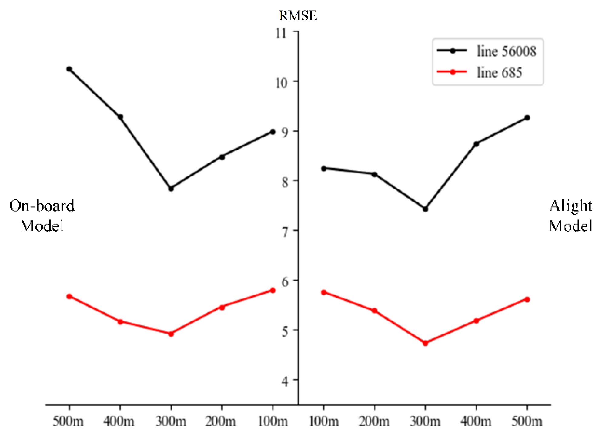
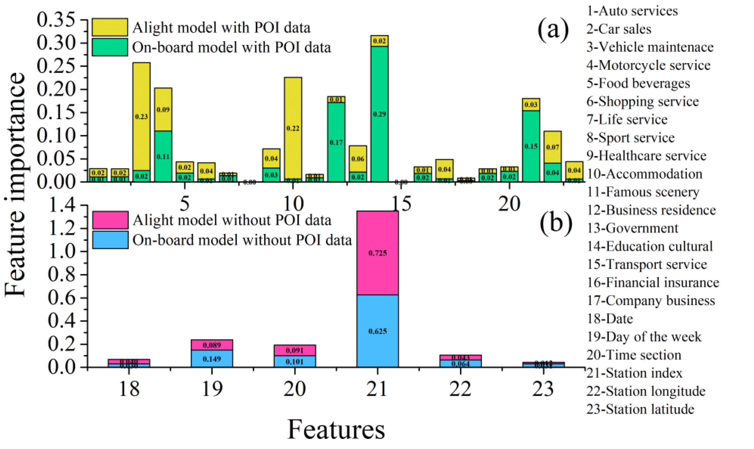
4.2. Impact Analysis of POI

There were 23 specific features selected in the PFP-XPOI model for passenger flow forecasting, and the feature importance is shown in Figure 7.

The times of node split were used as the feature importance in the XGBoost algorithm. The more times a feature splits, the more important it is. Figure 7 shows the feature importance of different models. PFP-XPOI uses the XGBoost algorithm to train the passenger flow prediction model. After the POI data are fused, the feature importance of the model will change significantly. When POI data are not used, the model mainly splits by the station index, which makes this feature significant in the split process. In the case of modeling with POI data, the model splits more evenly at different features.

The effect of the POI data on the passenger flow prediction for line 56008 is described directly in Figure 8 and Figure 9. They illustrate the predicted values of on-board and alighting passenger number from 7:00 to 7:30 on 29 October 2015. The predicted values of XGBoost and the historical average model are almost the same. According to this phenomenon, we can draw conclusions in accordance with the results shown in Figure 7. The major split point of the XGBoost model is the index of stations. After the calibration of the service radius between bus stations and POI data, the PFP-XPOI model has a better performance than other models in passenger flow prediction.

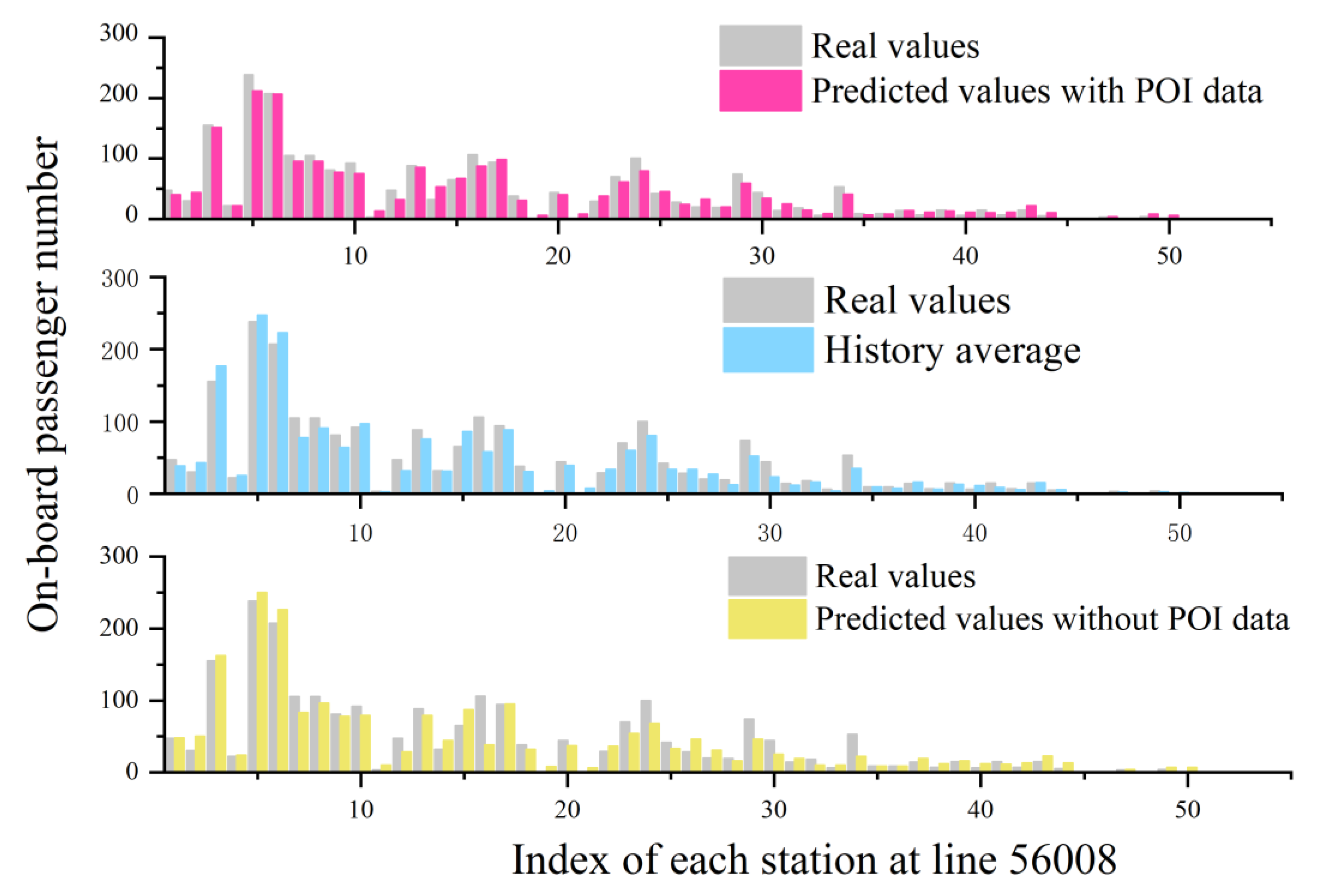
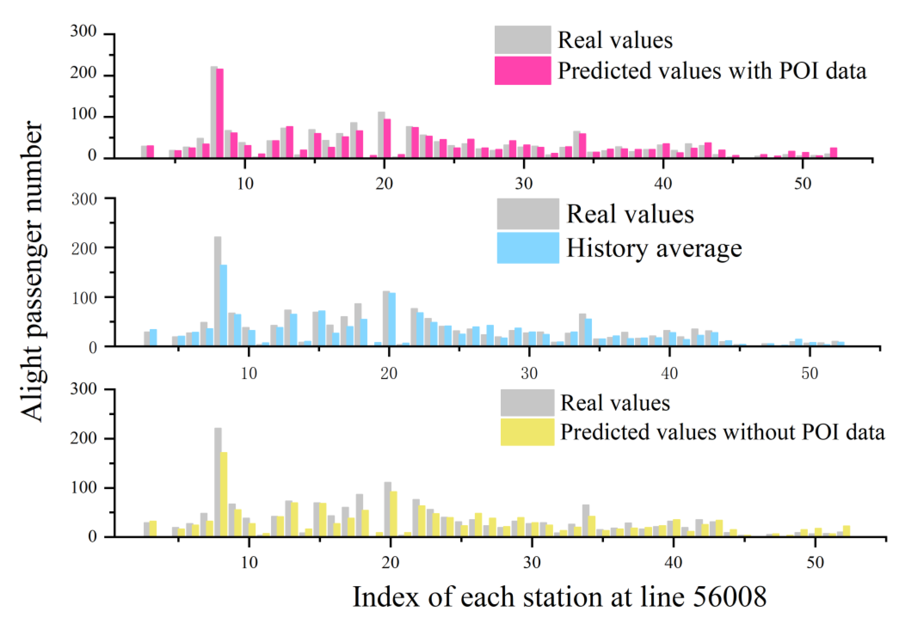
4.3. Comparison with Multiple Models

To verify the accuracy of the PFP-XPOI model, this study compared the performance of different models as listed in

Table 2. Evaluation values of different models for on-board passenger prediction in line 56008.

On-Board Passenger Prediction Models in Line 56008	RMSE	MAE	R-Squared
PFP-XPOI	7.84	7.32	0.912
XGBoost	8.79	8.16	0.889
LSTM	8.69	8.12	0.892
SVM	8.89	8.25	0.887
Historical Average	8.96	8.34	0.885

,

Table 3. Evaluation values of different models for alighting passenger prediction in line 56008.

Alighting Passenger Prediction Models in Line 56008	RMSE	MAE	R-Squared
PFP-XPOI	7.43	6.98	0.931
XGBoost	8.06	7.52	0.919
LSTM	7.49	7.13	0.929
SVM	7.96	7.48	0.921
Historical Average	8.12	7.65	0.917

,

Table 4. Evaluation values of different models for on-board passenger prediction in line 685.

On-Board Passenger Prediction Models in Line 685	RMSE	MAE	R-Squared
PFP-XPOI	4.92	4.53	0.890
XGBoost	5.76	4.74	0.849
LSTM	5.32	4.66	0.871
SVM	6.09	4.90	0.831
Historical Average	5.53	4.92	0.861

and

Table 5. Evaluation values of different models for alighting passenger prediction in line 685.

Alighting Passenger Prediction Models in Line 685	RMSE	MAE	R-Squared
PFP-XPOI	4.73	4.34	0.925
XGBoost	5.48	5.02	0.899
LSTM	5.13	4.97	0.912
SVM	5.53	5.12	0.898
Historical Average	5.69	5.14	0.892

. We used the RMSE, mean absolute error (MAE) and R-squared to evaluate different models. The MAE can be expressed as

$$\mathrm{MAE}=\frac{1}{M}{{\displaystyle \sum }}_{m=1}^M\left|y_m-{\widehat{y}}_m\right|$$

(12)

where M is the total number of samples. $y_m$ is the true value, and ${\widehat{y}}_m$ is the predicted value. R-squared can be expressed as

$$\mathrm{R}-\mathrm{squared}=1-\frac{{{\displaystyle \sum }}_{m=1}^M{\left(y_m-{\widehat{y}}_m\right)}^2}{{{\displaystyle \sum }}_{m=1}^M{\left(y_m-{\overline{y}}_m\right)}^2}$$

(13)

where M is the total number of samples. $y_m$ is the true value. ${\widehat{y}}_m$ is the predicted value, and ${\overline{y}}_{m }$ is the mean of samples.

Results reveal that the PFP-XPOI performs best, followed by LSTM and XGBoost. This phenomenon is similar to that obtained by Spyros Makridakis [16]. Because the alighting passenger flow is more stable, the alighting passenger flow prediction model is more accurate than the on-board passenger flow prediction model for both lines.

The results demonstrate that the PFP-XPOI model performs better in prediction and improves the prediction accuracy due to the addition of new features. The historical average data cannot effectively take the impact of week, POI and other factors into account so the error is relatively large. The error of using XGBoost model individually is similar to that of the historical mean. This also indicates that the direct application of XGBoost model for passenger flow prediction is mainly based on the station index.

5. Conclusions

Based on IC card data of Beijing buses, this study addressed the bus passenger flow prediction problem via fusing POI data by using the XGBoost algorithm. The proposed method takes advantage of the accuracy ensured by POI generated from bus operation data and the efficiency guaranteed by the XGBoost algorithm. Through the XGBoost algorithm, the big data of the bus card can be merged with the POI data. After calculating the experimental data, we chose “300 m” as the query radius because the prediction outcome is the most accurate. Due to some new added features, the PFP-XPOI model can improve the dimension of smart card data by fusing the POI data. By comparison and verification, it was proved that the proposed model has higher accuracy and runs faster.

This work may be further strengthened in other fields. The modeling of multiple buses arriving and leaving a single bus station would require more in-depth analysis. In the future, we will explore the applications of the proposed method in intelligent transportation system comprehensively.

References

1. Beijing Public Transport Corporation. Available online: http://www.bjbus.com/home/index.php (accessed on 23 December 2021).
2. Pelletier, M.P.; Trepanier, M.; Morency, C. Smart card data use in public transit: A literature review. Transp. Res. C-Emerg. 2011, 19, 557–568. [Google Scholar] [CrossRef]
3. Noekel, K.; Viti, F.; Rodriguez, A.; Hernandez, S. Modelling Public Transport Passenger Flows in the Era of Intelligent Transport Systems; Gentile, G., Noekel, K., Eds.; Springer Tracts on Transportation and Traffic; Springer International Publishing: Cham, Switzerland, 2016; Volume 1, ISBN 978-3-319-25080-9. [Google Scholar]
4. Zhai, H.W.; Cui, L.C.; Nie, Y.; Xu, X.W.; Zhang, W.S. A Comprehensive Comparative Analysis of the Basic Theory of the Short Term Bus Passenger Flow Prediction. Symmetry 2018, 10, 369. [Google Scholar] [CrossRef] [Green Version]
5. Iliopoulou, C.; Kepaptsoglou, K. Combining ITS and optimization in public transportation planning: State of the art and future research paths. Eur. Transp. Res. Rev. 2019, 11, 27. [Google Scholar] [CrossRef]
6. Milenkovic, M.; Svadlenka, L.; Melichar, V.; Bojovic, N.; Avramovic, Z. Sarima Modelling Approach for Railway Passenger Flow Forecasting. Transp.-Vilnius 2018, 33, 1113–1120. [Google Scholar] [CrossRef] [Green Version]
7. Li, Z.Y.; Bi, J.; Li, Z.Y. Passenger Flow Forecasting Research for Airport Terminal Based on SARIMA Time Series Model. In Proceedings of the IOP Conference Series: Earth and Environmental Science, Singapore, 22–25 December 2017; IOP Publishing Ltd.: Bristol, UK, 2017. [Google Scholar]
8. Ni, M.; He, Q.; Gao, J. Forecasting the Subway Passenger Flow Under Event Occurrences with Social Media. IEEE Trans. Intell. Transp. 2017, 18, 1623–1632. [Google Scholar] [CrossRef]
9. Tang, T.L.; Fonzone, A.; Liu, R.H.; Choudhury, C. Multi-stage deep learning approaches to predict boarding behaviour of bus passengers. Sustain. Cities Soc. 2021, 73, 103111. [Google Scholar] [CrossRef]
10. Wang, P.F.; Chen, X.W.; Chen, J.X.; Hua, M.Z.; Pu, Z.Y. A two-stage method for bus passenger load prediction using automatic passenger counting data. IET Intell. Transp. Syst. 2021, 15, 248–260. [Google Scholar] [CrossRef]
11. Ahmed, M.S.; Cook, A.R. Analysis of freeway traffic time-series data by using Box-Jenkins techniques. Transp. Res. Rec. 1979, 722, 1–9. [Google Scholar]
12. Li, L.C.; Wang, Y.G.; Zhong, G.; Zhang, J.; Ran, B. Short-to-medium Term Passenger Flow Forecasting for Metro Stations using a Hybrid Model. KSCE J. Civ. Eng. 2018, 22, 1937–1945. [Google Scholar] [CrossRef]
13. Gong, M.; Fei, X.; Wang, Z.H.; Qiu, Y.J. Sequential Framework for Short-Term Passenger Flow Prediction at Bus Stop. Transp. Res. Rec. 2014, 2417, 58–66. [Google Scholar] [CrossRef]
14. Ming, W.; Bao, Y.K.; Hu, Z.Y.; Xiong, T. Multistep-Ahead Air Passengers Traffic Prediction with Hybrid ARIMA-SVMs Models. Sci. World J. 2014, 2014, 567246. [Google Scholar] [CrossRef]
15. Sun, Y.X.; Leng, B.; Guan, W. A novel wavelet-SVM short-time passenger flowprediction in Beijing subway system. Neurocomputing 2015, 166, 109–121. [Google Scholar] [CrossRef]
16. Makridakis, S.; Spiliotis, E.; Assimakopoulos, V. Statistical and Machine Learning forecasting methods: Concerns and ways forward. PLoS ONE 2018, 13, e0194889. [Google Scholar] [CrossRef] [PubMed] [Green Version]
17. Liu, Y.; Liu, Z.Y.; Jia, R. DeepPF: A deep learning based architecture for metro passenger flow prediction. Transp. Res. C-Emerg. 2019, 101, 18–34. [Google Scholar] [CrossRef]
18. Ouyang, Q.; Lv, Y.B.; Ma, J.H.; Li, J. An LSTM-Based Method Considering History and Real-Time Data for Passenger Flow Prediction. Appl. Sci. 2020, 10, 3788. [Google Scholar] [CrossRef]
19. Yang, X.; Xue, Q.C.; Ding, M.L.; Wu, J.J.; Gao, Z.Y. Short-term prediction of passenger volume for urban rail systems: A deep learning approach based on smart-card data. Int. J. Prod. Econ. 2021, 231, 107920. [Google Scholar] [CrossRef]
20. Martinez-de-Pison, F.J.; Fraile-Garcia, E.; Ferreiro-Cabello, J.; Gonzalez, R.; Pernia, A. Searching Parsimonious Solutions with GA-PARSIMONY and XGBoost in High-Dimensional Databases. In Proceedings of the International Joint Conference SOCO’16-CISIS’16-ICEUTE’16, San Sebastian, Spain, 19–21 October 2016; Springer: Cham, Switzerland, 2017. [Google Scholar]
21. Nielsen, D. Tree Boosting with XGBoost—Why Does XGBoost Win "Every" Machine Learning Competition? Master’s Thesis, Norwegian University of Science and Technology, Trondheim, Norway, 2016. [Google Scholar]
22. Dong, X.C.; Lei, T.; Jin, S.T.; Hou, Z.S. Short-Term Traffic Flow Prediction Based on XGBoost. In Proceedings of the 2018 IEEE 7th Data Driven Control and Learning Systems Conference, Enshi, China, 25–27 May 2018. [Google Scholar]
23. Lee, E.H.; Kim, K.; Kho, S.Y.; Kim, D.K.; Cho, S.H. Estimating Express Train Preference of Urban Railway Passengers Based on Extreme Gradient Boosting (XGBoost) using Smart Card Data. Transp. Res. Rec. 2021, 2675, 64–76. [Google Scholar]
24. Aslam, N.S.; Ibrahim, M.R.; Cheng, T.; Chen, H.F.; Zhang, Y. ActivityNET: Neural networks to predict public transport trip purposes from individual smart card data and POIs. Geo-Spat. Inf. Sci. 2021, 24, 711–721. [Google Scholar] [CrossRef]
25. Faroqi, H.; Mesbah, M. Inferring trip purpose by clustering sequences of smart card records. Transp. Res. C-Emerg. 2021, 127, 103131. [Google Scholar] [CrossRef]
26. Bao, J.; Xu, C.C.; Liu, P.; Wang, W. Exploring Bikesharing Travel Patterns and Trip Purposes Using Smart Card Data and Online Point of Interests. Netw. Spat. Econ. 2017, 17, 1231–1253. [Google Scholar] [CrossRef]
Figure 1. The process and organization of the PFP-XPOI model.
Applsci 12 00940 g001
Figure 2. The RMSE and distance of passenger number prediction model in lines 56008 and 685.
Applsci 12 00940 g002
Figure 3. Prediction and true values of on-board passenger number for line 56008.
Applsci 12 00940 g003
Figure 4. Prediction and true values of alighting passenger number for line 56008.
Applsci 12 00940 g004
Figure 5. Prediction and true values of on-board passenger numbers for line 685.
Applsci 12 00940 g005
Figure 6. Prediction and true values of alighting passenger numbers for line 685.
Applsci 12 00940 g006
Figure 7. The feature importance of different XGBoost models with POI data (a) and without POI data (b).
Applsci 12 00940 g007
Figure 8. Predicted and true values of on-board passenger numbers using three models.
Applsci 12 00940 g008
Figure 9. Predicted and true values of alighting passenger numbers using three models.
Applsci 12 00940 g009