A Surrogate-Model-Based Approach for the Optimization of the Thermal Design Parameters of Space Telescopes

Abstract

The thermal design parameters of space telescopes are mainly optimized through traversal and iterative attempts. These optimization techniques are time consuming, rely heavily on the experience of the engineer, bear a large computational workload, and have difficulty in achieving optimal outcomes. In this paper, we propose a design method (called SMPO) based on an improved back-propagation neural network (called GAALBP) that builds a surrogate model and uses a genetic algorithm to optimize the model parameters. The surrogate model of a space telescope that measures the atmospheric density is established using GAALBP and then compared with surrogate models established using a traditional BP neural network and radial-basis-function neural network. The results show that the regression rate of the surrogate model based on the GAALBP reaches 99.99%, a mean square error of less than 2 × 10⁻⁶, and a maximum absolute error of less than 4 × 10⁻³. The thermal design parameters of the surrogate model are optimized using a genetic algorithm, and the optimization results are verified in a finite element simulation. Compared with the design results of the manually determined thermal design parameters, the maximum temperature of the CMOS is reduced by 5.33 °C, the minimum temperature is increased by 0.39 °C, and the temperature fluctuation is reduced by a factor of 4. Additionally, SMPO displays versatility and can be used in various complex engineering applications to provide guidance for the better selection of appropriate parameters and optimization.

1. Introduction

Space telescopes are developing toward deep space exploration and maneuver to change orbit, with increasing demands on imaging quality, however, they experience changing and complex thermal environments [1,2]. The temperature of a telescope directly affects its imaging quality, and a reliable thermal design remains the basis for ensuring the stable operation of the telescope [3]. The thermal design of telescopes involves the iterative optimization of a large number of parameter combinations, which currently relies on the design experience of engineers and involves a process of repeated attempts. The process is time consuming and it is difficult to find an optimal solution. The development of methods that allow the rapid optimization of the thermal design parameters of telescopes has become an important issue [4], and techniques of parameter optimization have thus received much attention in recent years.

Scholars have investigated the parameter optimization of space telescopes, but there have been few studies on the optimization of the thermal design parameters of space telescopes. As examples, del Rio et al. [5] optimized the design parameters of X-ray mirrors using a genetic algorithm (GA) and Zhang et al. [6] used the inverse of the effective temperature of a star for a given flux density obtained using a stochastic particle swarm optimization algorithm and angular parameters, and solved the problem where the band-pass density of the detector is determined and fixed during the operational phase. Popular parametric optimization methods such as particle swarm algorithms [7,8] and genetic algorithms [9,10] reveal a better optimization speed and performance than the iterative trial-and-error approach that relies on the engineer. Among these methods, a GA as a global optimization probabilistic algorithm is employed to find an optimal value on the basis of superiority and inferiority and adapts to arbitrary forms of objective functions and constraints. Therefore, GA shows great potential and advantages in the design of thermal parameters of future complex space telescopes. However, these optimization algorithms are combined with traditional physical models to conduct finite element iterative calculations after selecting parameter combinations, which is a time-consuming process of solving partial differential equations that greatly reduces the speed of parameter optimization. The technique of using a surrogate model has attracted attention in recent years for its ability to accelerate the parameter optimization iterations and ensure the accuracy of design at the same time.

A surrogate model [11,12,13] is commonly used for optimization in engineering problems. When the actual problem (involving a high-precision model) is computationally intensive and difficult to solve, a simplified model that is less computationally intensive and fast to solve can be used in place of the original model to accelerate optimization. The surrogate models most commonly used are those of the kriging method [13], polynomial response surface method [14], and artificial neural network [15], which have various industrial applications, including the thermal design of spacecraft. A back-propagation (BP) neural network [16,17] is a multilayer feedforward network that can express almost any nonlinear system and is widely used in various fields owing to its excellent fitting ability. As examples, Cui et al. [18] established a three-component proxy ignition delay prediction model based on a BP neural network, which had a computational speed that was nearly 9 times that of the traditional ignition delay calculation, and Zhao et al. 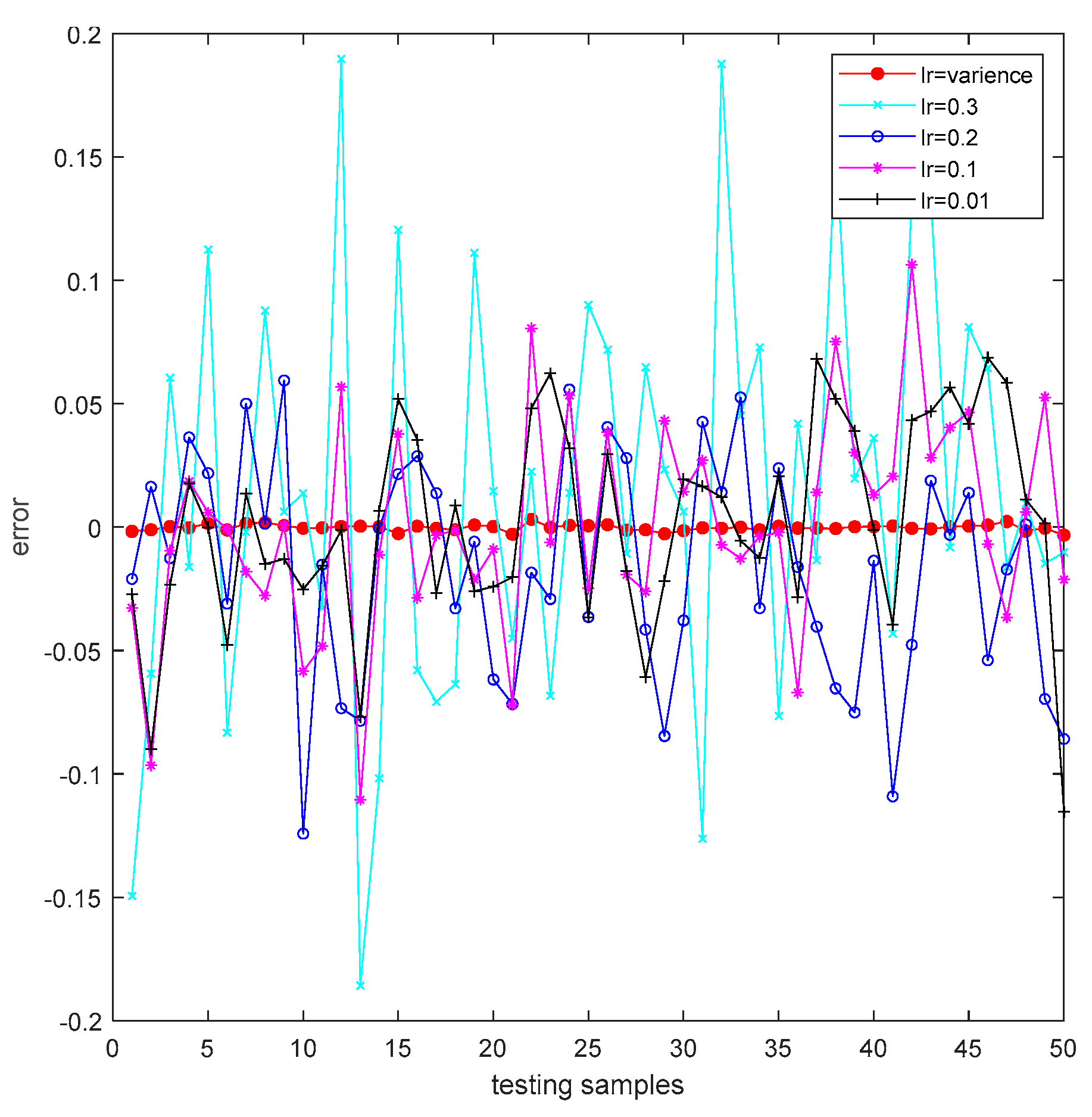[19] proposed a surrogate model for computational fluid dynamics simulation based on a GA–BP neural network to predict the concentration of aerosols after diffusion, which solved the problem of the simulation not being achieved in real time when predicting the concentration of diffused gas. Although the BP neural network has a good fitting effect, the setting of the network hyperparameters significantly affects the fitting efficiency and accuracy of the network. The learning rate, initial weights, and thresholds are the parameters that most affect the network performance. The learning rate of the traditional BP network is fixed, regardless of the magnitude of error, always with a fixed learning rate to adjust the weights, etc. If the learning rate is too high, it may not be possible to directly cross the global optimum resulting in a failure to converge. If the learning rate is too low, the loss function changes slowly, there is a large increase in the convergence complexity of the network, and the process is easily trapped in local extremes. In addition, the neural network requires constant iterative updating of weights and thresholds during the computation to perform well [20,21]. The initialization of weights and thresholds of traditional BP networks is randomly generated, and during the training process, phenomena such as gradient disappearance and gradient explosion are often encountered. Therefore, proper initialization of the weights can effectively avoid these two issues and improve the model performance and convergence speed.

On the basis of the above analysis, this paper proposes a design method (called SMPO) that uses an improved BP neural network (called GAALBP) to establish a telescope surrogate model and optimizes the model parameters using a GA to optimize the thermal design of a telescope. GAALBP employs a GA to optimize the initial network weights and thresholds, and the learning rate adaptively changes with the error during the training, allowing for the training of a better surrogate model and providing a physical basis for subsequent parameter optimization. The remainder of this paper is organized as follows: Section 2 details the proposed design methodology of SMPO. Section 3 describes the application of SMPO to the parameter optimization of the thermal design parameters for a space telescope and compares the results with those obtained using the traditional method of manual parameter optimization. Section 4 presents the conclusions of the study.

2. Methodology of SMPO

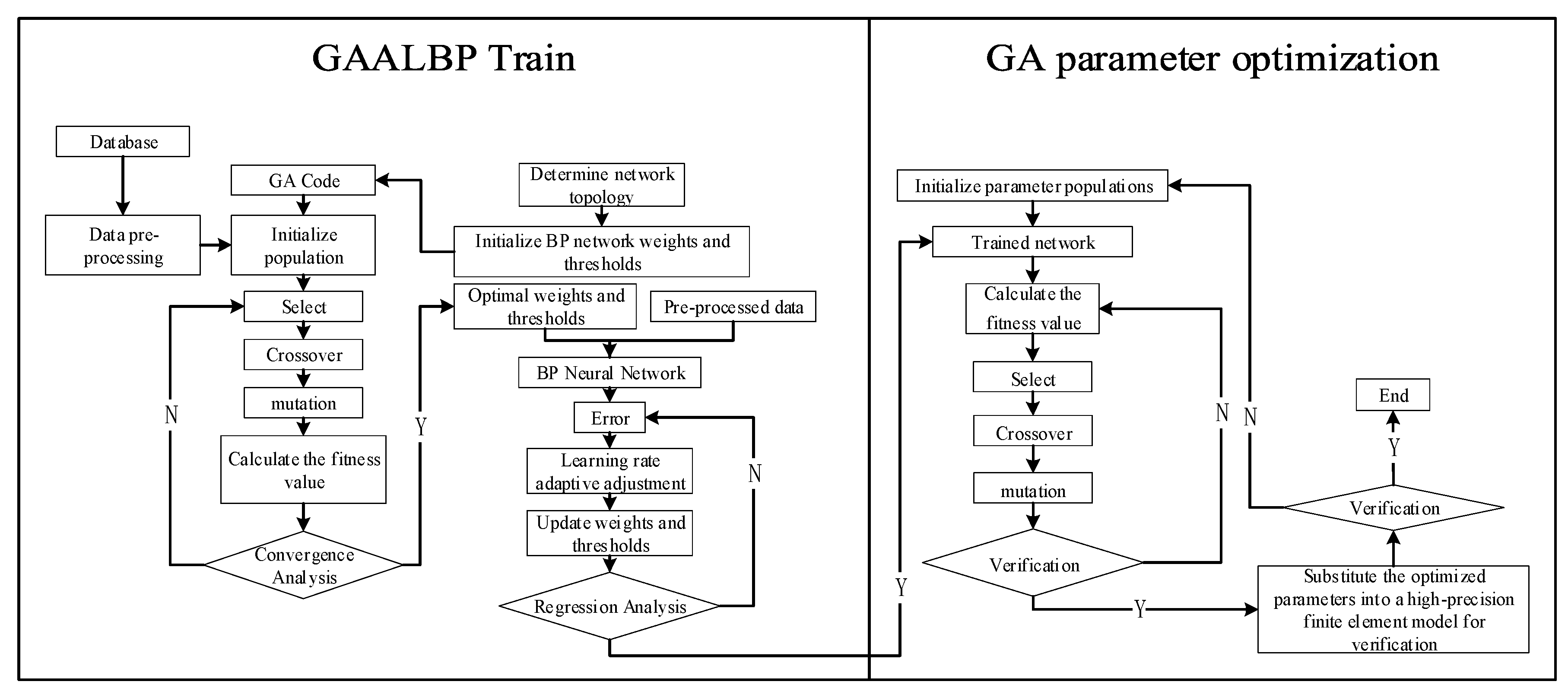
The methodology of SMPO involves building a surrogate model using GAALBP and using a GA to find the best parameters, as shown in Figure 1.

Figure 1. SMPO flow chart.

Part I: GAALBP network training

This paper proposes an improved BP neural network. The improved network uses a GA to optimize the initial weights and thresholds of the network, the best individuals in the population are selected in a winner-takes-all manner [22], and the coding information of the best individuals is used for the initial weights and thresholds of the network. Therefore, before the training of the network, the GA coding length and fitness value need to be calculated and data preprocessing conducted. The calculations are as follows:

(1) Calculation of the encoding length. The length S of the GA encoding is derived from the network topology determined by the feature dimensions of the input and output and the numbers of layers and nodes of the hidden layer. The calculation is

$$S=(n_{in}+1)\times n_1+\left({\displaystyle \sum _{i=1}^{N-1}\left((n_i+1)\times n_{i+1}\right)}\right)+(n_N+1)\times n_{out}$$

(1)

where n_in is the number of neurons in the input layer, N is the number of layers in the hidden layer, n_i is the number of neurons in the hidden layer (i = 1, 2,…, N), and n_out is the number of neurons in the output layer.

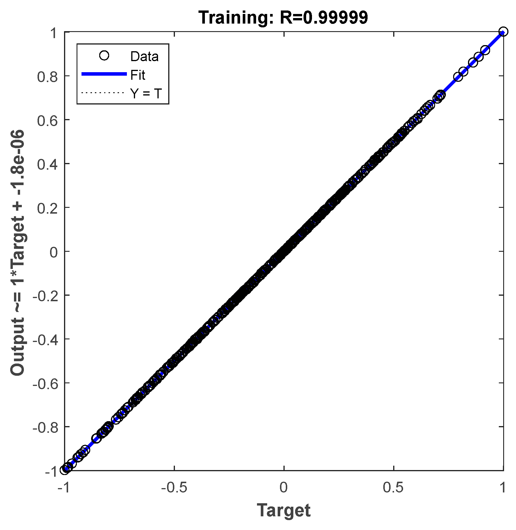
(2) Calculation of the fitness value. In the training phase of the network, the mean square deviation of the predicted values fitted to the network from the true values is taken as the fitness value of the GA. The maximum fitness value is zero when T_real and T_pre are equal. The calculation is

$$fitness=-\frac{{\displaystyle \sum _{i=1}^N\left|T_{reali}-T_{prei}\right|}}{N}$$

(2)

where T_prei is the predicted temperature, T_reali is the true temperature, and N is the number of test samples.

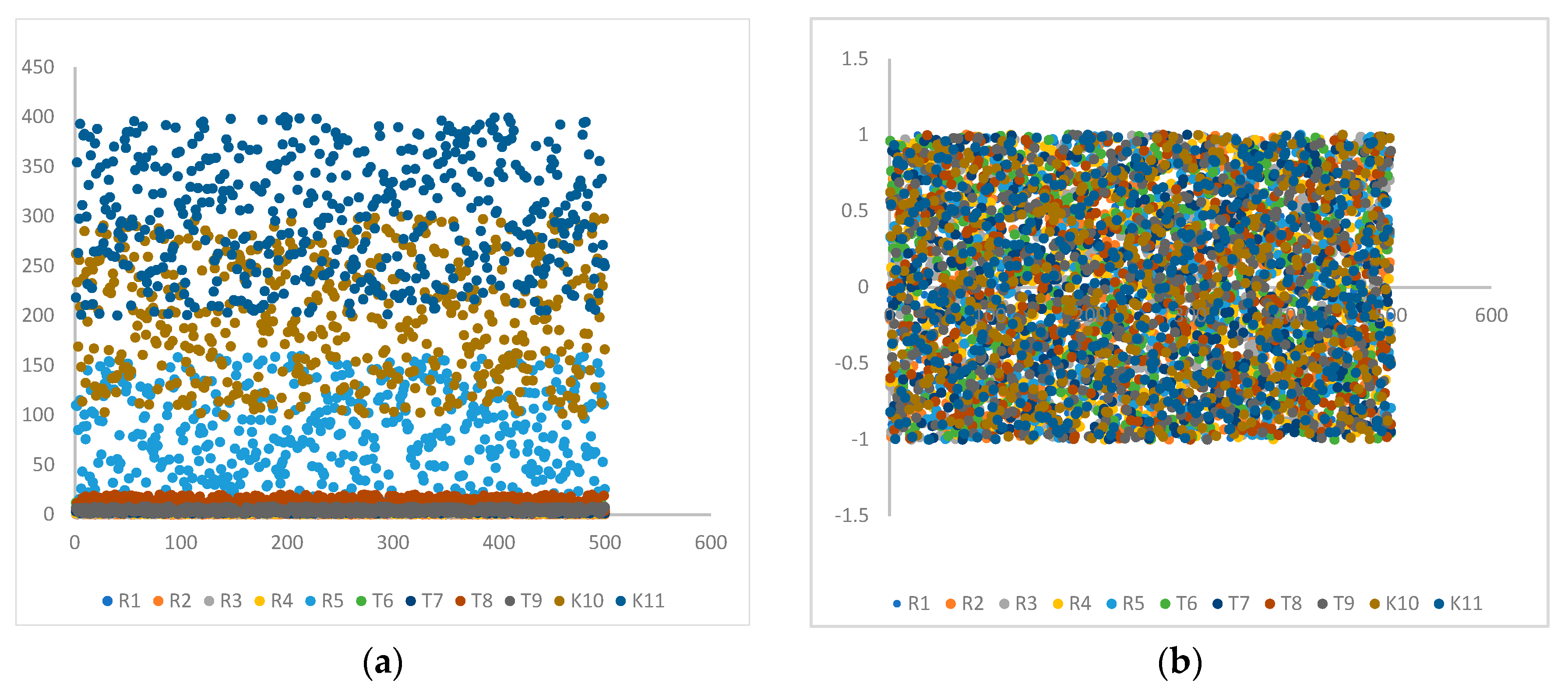
(3) Data preprocessing. The input data are normalized to eliminate the effect of variables of different orders of magnitude on the network training. Here, the optimal normalization method [23] is used to map the data to the range [−1, 1]. The calculation is

$$y=\frac{2\times \left(x-x_{\min }\right)}{x_{\max }-x_{\min }}-1$$

(3)

where x_min is the minimum value for the same dimension, and x_max is the maximum value for the same dimension.

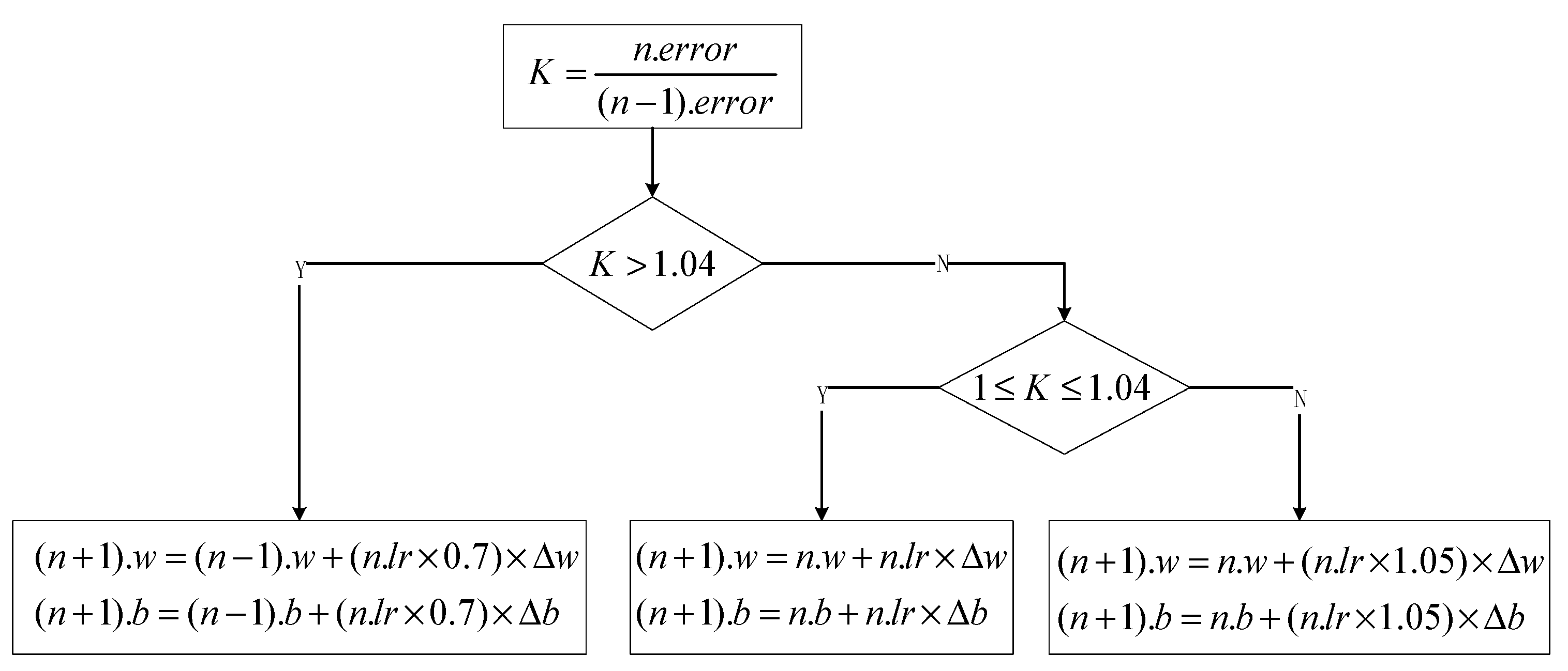
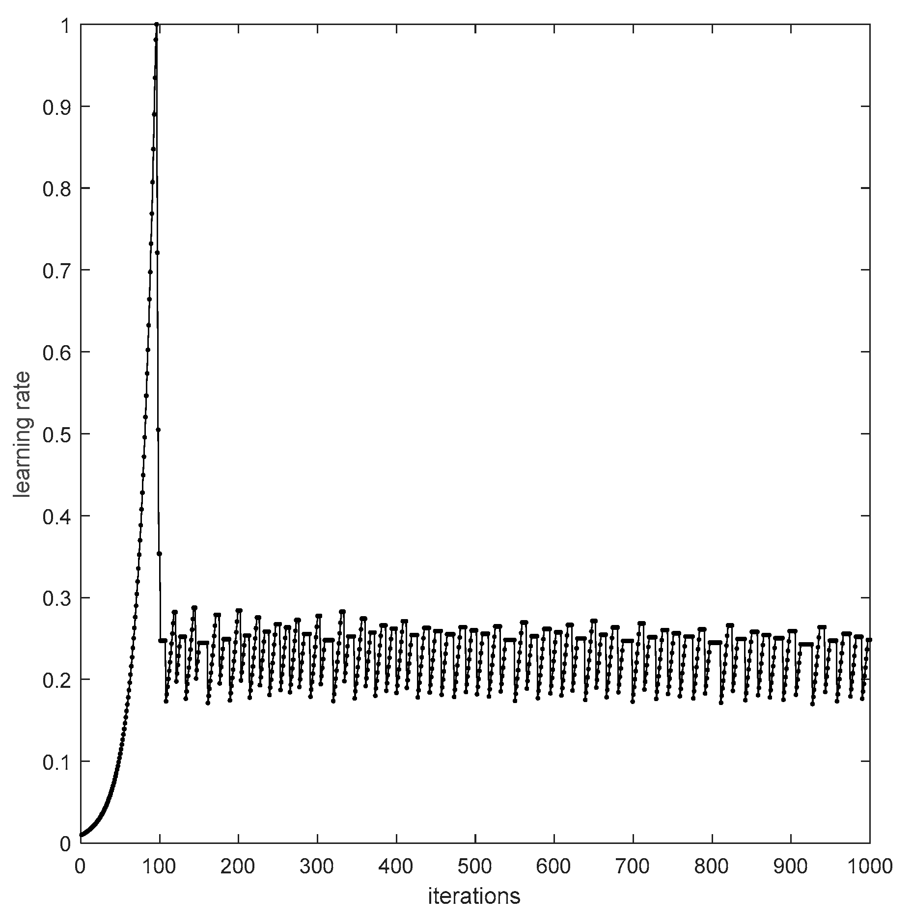
The optimized weights and thresholds are assigned to the BP network, and the input data are used to train the network. During the training process, the learning rate changes adaptively with the relative change in the error, bearing the aim of keeping the learning stable while maintaining the largest possible learning step. If the error increases, a smaller learning rate is used in continuously searching for the direction of the gradient descent, and if the error increases by more than a certain percentage, the weights and thresholds of the previous round are discarded and the learning rate is reduced. This process improves the learning rate, however, when the learning rate is too high and the error reduction is not guaranteed, the learning rate is reduced until stable learning is restored. The improved BP network compensates for drawbacks such as the fixed learning rate of the BP network and can be trained to obtain a better surrogate model. The rule for correcting the learning rate with error is determined by manual debugging, and the method of adaptively adjusting the learning rate is shown in Figure 2. If the error in the current round increases by more than a factor of 1.04 relative to that in the previous round, the weights and thresholds of the current round are discarded, and the weights and thresholds in the next round are calculated using the values of the previous round, and the learning rate is reduced by a factor of 0.7. If the error in the current round is higher than that in the previous round but by less than a factor of 1.04, then the current weights, thresholds, and learning rate are retained. If the error continues to decrease, the learning rate is increased by a factor of 1.05.

Figure 2. Flowchart of the adaptive adjustment of the learning rate.

In Figure 2, n.error is the error in round n, (n − 1).error is the error in round (n − 1); n.w and n.b are, respectively, the weight and threshold in round n; (n + 1).w and (n + 1).b are, respectively, the weight and threshold in round (n + 1); and ∆w, ∆b is the variation calculated from the error using the gradient descent method.

Part II: GA parameter optimization

The GA is used to find the output extrema of the established surrogate model and the optimal solution corresponding to the extrema.

The GA initializes the generated population in the given parameter ranges. By setting the target output value, in the stage of seeking the extreme value, the difference between the target value and the actual output value is found and the negative of its absolute value is used as the fitness value fit of the GA, and the optimal solution is obtained by selecting the optimal individuals through crossover and mutation operations. Finally, the optimization result is substituted into the high-precision finite element model to verify whether the output satisfies the demand, and if not, the number of population individuals are increased iteratively until the target is met. The fitness value fit is calculated as

$$fit=-\left|T_{real}-T_{pre}\right|$$

(4)

where T_pre is the predicted temperature and T_real the true temperature.

3. Example Applications and Results

To verify its performance, SMPO is applied in the optimization of the thermal design parameters of an atmospheric density measurement space telescope (called the ADST), which was designed and manufactured in China, and the optimized parameters are substituted into high-precision finite element software for verification. A comparison is made with the results of the current conventional method of relying on an engineer’s experience to optimize the design using the solving of partial differential equations, and the superiority of the optimization framework is thus verified.

3.1. Background of the ADST

The atmospheric density measurement space telescope (ADST) is tasked with monitoring the density of the stratospheric atmosphere at an orbital height of 280 km and an orbital inclination of 90°. The ADST primarily includes a main frame, filter wheel assembly, mirror barrel, and detector-focal-plane assembly (including a complementary metal–oxide–semiconductor (CMOS) detector and CMOS board and two circuit boards with field-programmable gate arrays). The thermophysical finite element model of the ADST was developed using a nodal network [24] as shown in Figure 3. The internal heat source mainly reflects the heat generation of the CMOS of the ADST. The CMOS works intermittently (twice per track) with a power consumption of 1 W and has a preparation time less than 10 min and working time of less than 5 min. The heat consumption of the internal heat source is the same for the preparation state and working state. High- and low-temperature conditions and thermal control indicators are defined in Table 1 and Table 2. The ADST telescope is installed inside the module, and only the light inlet is in contact with the space environment. The heat generated by the internal consumption of the ADST is not directly exchanged with the external environment, and the CMOS is extremely sensitive to temperature fluctuations. In this paper, SMPO is applied to optimize the thermal design parameters of the ADST telescope and thus control the temperature of the ADST.

Figure 3. Finite element model of the ADST.

Table 1. Definitions of high- and low-temperature cases for the ADST.

Cases	Definition of Cases
High Case	ADST initial temperature 28 °C; due to the variable interval, the high case is analyzed according to 2 times continuous working, i.e., 30 min continuous working.
Low Case	ADST initial temperature 10 °C; internal heat source does not work; platform temperature control circuit works for a long time, other thermal control works 2 times per track, single work for 15 min, interval 30 min.

Table 2. Thermal control index of the ADST.

	Index
	Low Case	High Case
CMOS	>10 °C	≤40 °C (Fluctuations < 10 °C)
Main frame	>10 °C	≤35 °C

The CMOS works intermittently inside the cabin, and the heat generated by internal consumption is not exchanged directly with the external environment. After the preliminary thermal design, it was proposed to install the ADST adiabatically with its surrounding components. The surface of the ADST is blackened to reduce the effect of the cabin environment and other components on the temperature of the ADST. The heat generated by the CMOS is then transferred to the main frame through heat conduction and other means to achieve its temperature control. The heat transfer path of the CMOS is shown in Figure 4. The present paper takes the temperature of the ADST as the optimization target and selects 11 main thermal design parameters of the heat dissipation path as the parameters to be optimized, as shown in Table 3. The proposed SMPO is then used to control the temperature of the ADST.

Figure 4. CMOS heat transfer path.

Table 3. Parameters to be optimized.

	Parameter	Detail	Unit	Minimum Value	Maximum Value
Thermal resistance	R1	CMOS- Heat conductive block	°C/W	1	8
	R2	Heat conductive block -Copper1	°C/W	0	0.8
	R3	Copper1-Copper2	°C/W	0.2	4
	R4	Copper2- Main frame	°C/W	0.4	5
	R5	CMOS- Installation plate	°C/W	10	160
Thickness	T6	Heat conductive block	mm	3	12
	T7	Copper	mm	1	6
	T8	Main frame	mm	3	20
	T9	Installation plate	mm	0.6	8
Thermal conductivity	K10	Heat conductive block	W/(m∙K)	100	300
	K11	Copper	W/(m∙K)	200	400

3.2. Application of SMPO

Before being imported into the surrogate model for training, the data need to be normalized to eliminate the effects of variables of different orders of magnitude on the training results. The present paper adopts most-valued normalization to map the original data to the range of [−1, 1] according to Equation (2). The data distributions before and after the normalization are shown in Figure 5. It is observed that the normalized data distribution is more concentrated and contains a smaller difference between the variables, which are conducive to accelerating the convergence of the update of the network training weights.

Figure 5. Comparison of the distribution of data before and after normalization ((a). Data before normalization; (b). Data after normalization).

The normalized data are imported into the GAALBP network, with 90% of the data used for training and 10% for testing. Eleven parameters are optimized as inputs and the predicted temperature of the CMOS is taken as the output. Hyperparameters of the network are set as presented in Table 4. Hyperparameters are mainly divided into GAALBP network hyperparameters and hyperparameters of the GA that optimize the initialization weights and thresholds of the network. The training process and results are shown in Figure 6 and Figure 7, where it is seen that, the network training regression rate reaches 0.9999 and the maximum prediction error (the difference between the predicted value and true value) of the network is less than 4 × 10⁻³. The adaptive learning rate during training is shown in Figure 8. At the beginning of training, the learning rate continually increases, indicating that the error is gradually decreasing. In the later stages of training, the learning rate fluctuates around a value of 0.2, indicating that the training error has increased. However, the learning rate displays an overall decreasing trend, indicating that the training error decreases. The training effects of the adaptive learning rate and the improved BP network are compared for constant learning rates of 0.01, 0.1, 0.2, and 0.3, as shown in Figure 9. The test error for the adaptive learning rate is two orders of magnitude smaller than the test errors for the constant learning rates when the hyperparameters are the same, demonstrating the superiority of the adaptive learning rate.

Table 4. Network hyperparameter settings.

	Hyperparameter	Detail	Value
1	nin	Number of neurons in the input layer of the network	11
2	nout	Number of neurons in the output layer of the network	1
3	lrBase	Network initial learning rate	0.01
4	lrInc	Learning Rate Growth Rate	1.04
5	lrDec	Learning rate decline rate	0.7
6	epochs	Maximum rounds	1000
7	popSize	GA population size	50
8	maxTerm	Maximum iterations of GA	100

Figure 6. Network training regression rate.

Figure 7. Network prediction error.

Figure 8. Learning rate change curve.

Figure 9. Training error for different learning rates.

The quality of the surrogate model directly determines how well the parameters are optimized in the subsequent step. Comparisons are made with the traditional BP network, GA-optimized BP (GABP) network, and radial basis function neural network [25] to verify the superiority of GAALBP. The training results are presented in Table 5 and Figure 10. The GABP network is a BP network with a GA-optimized constant learning rate; i.e., the only difference between the GABP and GAALBP is the difference in the learning rate variation. It is seen that the training error of GAALBP is 1% of that of the traditional BP network and 40% that of the GABP network whereas the mean square error of GAALBP is smaller than the mean square errors of the other networks. The results thus demonstrate the superiority of GAALBP.

Table 5. Comparison of prediction errors of different networks.

	BP	RBF	GABP	GAALBP
Regression rate	0.89955	0.9693	0.9824	0.9999
MSE Error	0.065456	1.224 × 10−4	2.5496 × 10−6	1.9451 × 10−6
Maximum Error	0.4	0.25	0.01	4 × 10−3

Figure 10. Prediction errors of different networks.

After establishing the surrogate model, the GA is used to optimize the input of the surrogate model to meet the thermal control index of the CMOS. The negative of the absolute value of the difference between the target temperature and predicted temperature is taken as the fitness value of GA training:

$$fit=-\left|T_{goal}-T_{pre}\right|$$

(5)

where T_goal is the target temperature and T_pre is the predicted temperature. A larger fitness value means that the predicted temperature is closer to the target temperature, meaning that the parameter optimization is better.

The GA hyperparameters are set as given in Table 6. The coding length of genetic individuals is equal to the number of parameters to be optimized (i.e., 11), and each individual coding contains all the information of the parameters to be optimized. The size of the initialized population is 100. The individuals are input to the surrogate model to calculate the fitness value, and the poorly adapted individuals are eliminated in the manner of survival of the fittest. Meanwhile, the highly adapted individuals are crossed and mutated to produce new individuals. New rounds of iterations are performed until the best adapted individuals in the population are selected.

Table 6. GA hyperparameter settings.

	Hyperparameters	Detail	Value
1	PopSize	Population size	100
2	MaxTerm	Maximum iterations	100
3	Method of Mutation	mutation	boundaryMutation
4	Method of Select	Select	normGeomSelect
5	Method of Crossover	Crossover	heuristicXover

One-hundred iterations are performed. The iterative process is presented in Table 7. The algorithm selects the best individual as having a fitness value of −0.0002, indicating that the difference between the temperature of the optimized CMOS and the CMOS index is not greater than 0.0002.

Table 7. GA iterative process.

	p1	p2	p3	p4	p5	p6	p7	p8	p9	p10	p11	Fitness
1	7.2	0.620	3.175	1.72	40.39	5.910	5.61	19.3	5.08	223.8	341	−9.284
2	2.5	0.143	2.805	1.63	42.44	3.997	2.63	5.59	6.69	133.0	235	−4.404
3	1.5	0.087	1.971	3.13	156.4	6.376	5.02	5.59	6.59	265.2	371	−7.119
4	4.3	0.724	1.189	2.58	98.98	5.969	3.69	5.64	6.53	231.1	381	−11.055
5	6.8	0.701	2.363	2.09	55.66	6.078	3.31	4.52	5.84	209.2	392	−2.1866
…	…	…	…	…	…	…	…	…	…	…	…	…
99	2.5	0.214	1.178	1.47	40.68	6.065	3.01	11.99	1.81	129.2	304	−0.0002
100	2.5	0.214	1.178	1.47	40.68	6.065	3.01	11.99	1.81	129.2	304	−0.0002

To verify the optimized results, the parameters optimized by the GA are substituted into software for Monte Carlo simulation using the finite element method for thermal design, and the optimized results are verified for the high- and low-temperature cases of the telescope. The verification results are presented in Figure 11, Figure 12 and Figure 13. Figure 11a shows the temperature cloud of the CMOS heat dissipation component in the low-temperature case whereas Figure 11b shows the temperature cloud of the CMOS itself in the low-temperature case. Figure 12a shows the temperature cloud of the CMOS heat dissipation component in the high-temperature case whereas Figure 12b shows the temperature cloud of the CMOS itself in the high-temperature case. Figure 13 shows the temperature fluctuation of the CMOS itself in the high- and low-temperature cases. The figures reveal that in the low-temperature case, as the internal heat source essentially fails to work and the CMOS package in the cabin is less affected by external heat flow, the overall minimum temperature of the CMOS components exceeds 10 °C, the maximum temperature is less than 13.9 °C, the temperature of the CMOS itself is stable at 12.82 °C, and the temperature uniformity is within 0.01 °C. In the high-temperature case, the internal heat source works intermittently, the overall temperature uniformity of the CMOS components is within 0.93 °C, the minimum temperature of the CMOS itself is 31.10 °C, the maximum temperature is 32.69 °C, and the maximum temperature fluctuation is less than 1.6 °C, which meets the demands of the CMOS thermal control index.

Figure 11. Temperature clouds of CMOS components in the low-temperature case ((a). Heat dissipation component; (b). CMOS).

Figure 12. Temperature clouds of CMOS components in the high-temperature case ((a). Heat dissipation component; (b). CMOS).

Figure 13. CMOS temperature fluctuations in the high- and low-temperature cases.

3.3. Results

The optimization results of SMPO are compared with the results of the manual optimization of CMOS thermal parameters by engineers as presently performed in industry to verify the performance of SMPO. Additionally, the optimized results are substituted into finite element software to verify the performance of the parameters in the high- and low-temperature cases. The results are shown in Figure 14. In the low-temperature case, CMOS components essentially fail to work, there is no internal heat source, the CMOS temperature basically does not fluctuate, and the results obtained through SMPO optimization and those obtained through manual optimization both meet the requirements of the CMOS thermal control index, however, the overall temperature in the results obtained through SMPO is 0.5 °C higher than that in the results obtained through manual optimization, leaving a greater temperature margin in the low-temperature case. In the high-temperature case, the internal heat source works intermittently. Compared with the results obtained through manual optimization, the temperature derived through SMPO is 5.33 °C lower at the highest temperature of the CMOS and 0.39 °C lower at the lowest temperature of the CMOS. Additionally, the temperature fluctuation is reduced by a factor of 4, and the calculation time is reduced from several days to a few hours. The effectiveness and superiority of SMPO are thus demonstrated.

Figure 14. Comparison of the performance of parameter optimization in high- and low-temperature cases.

4. Conclusions

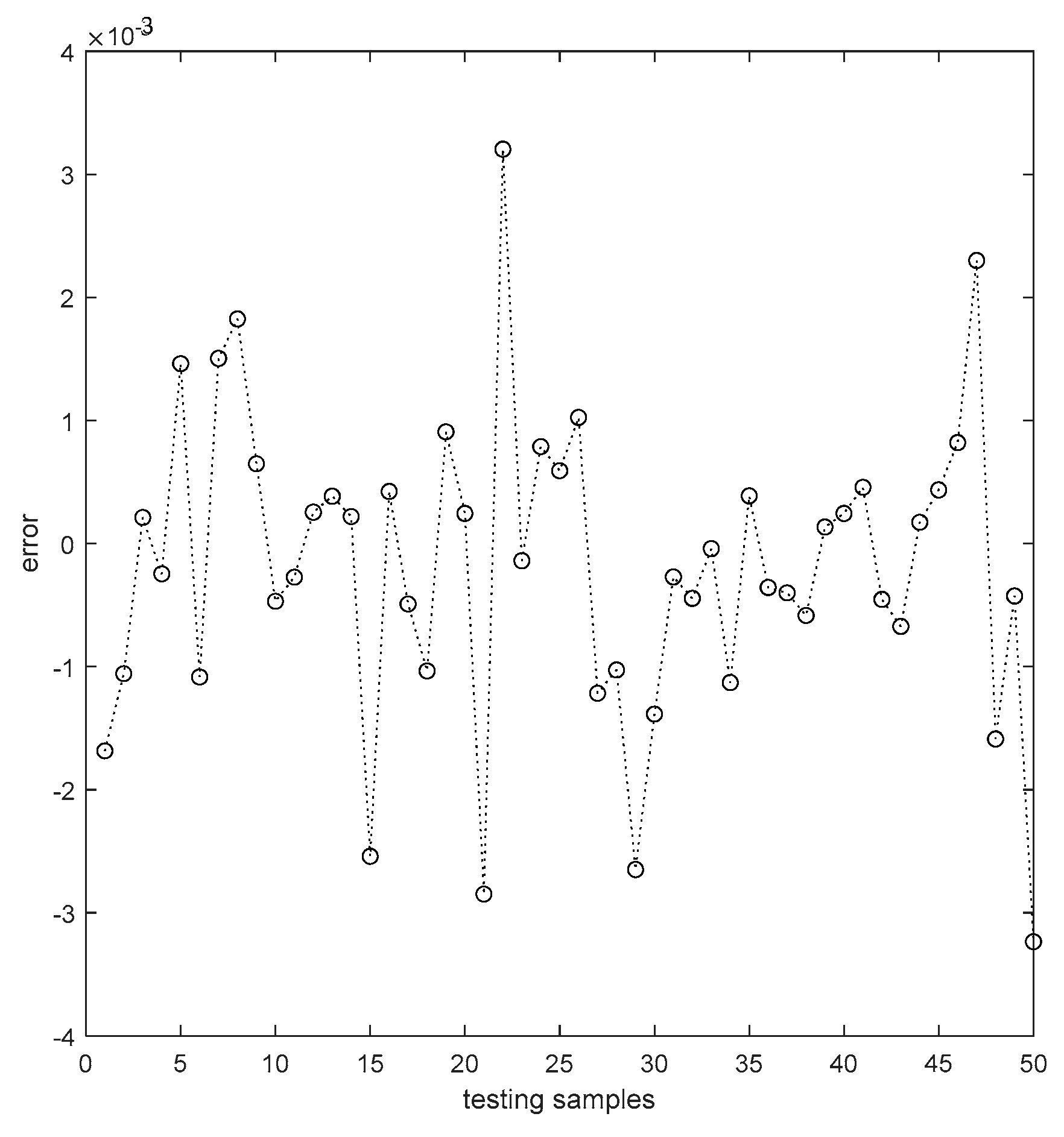
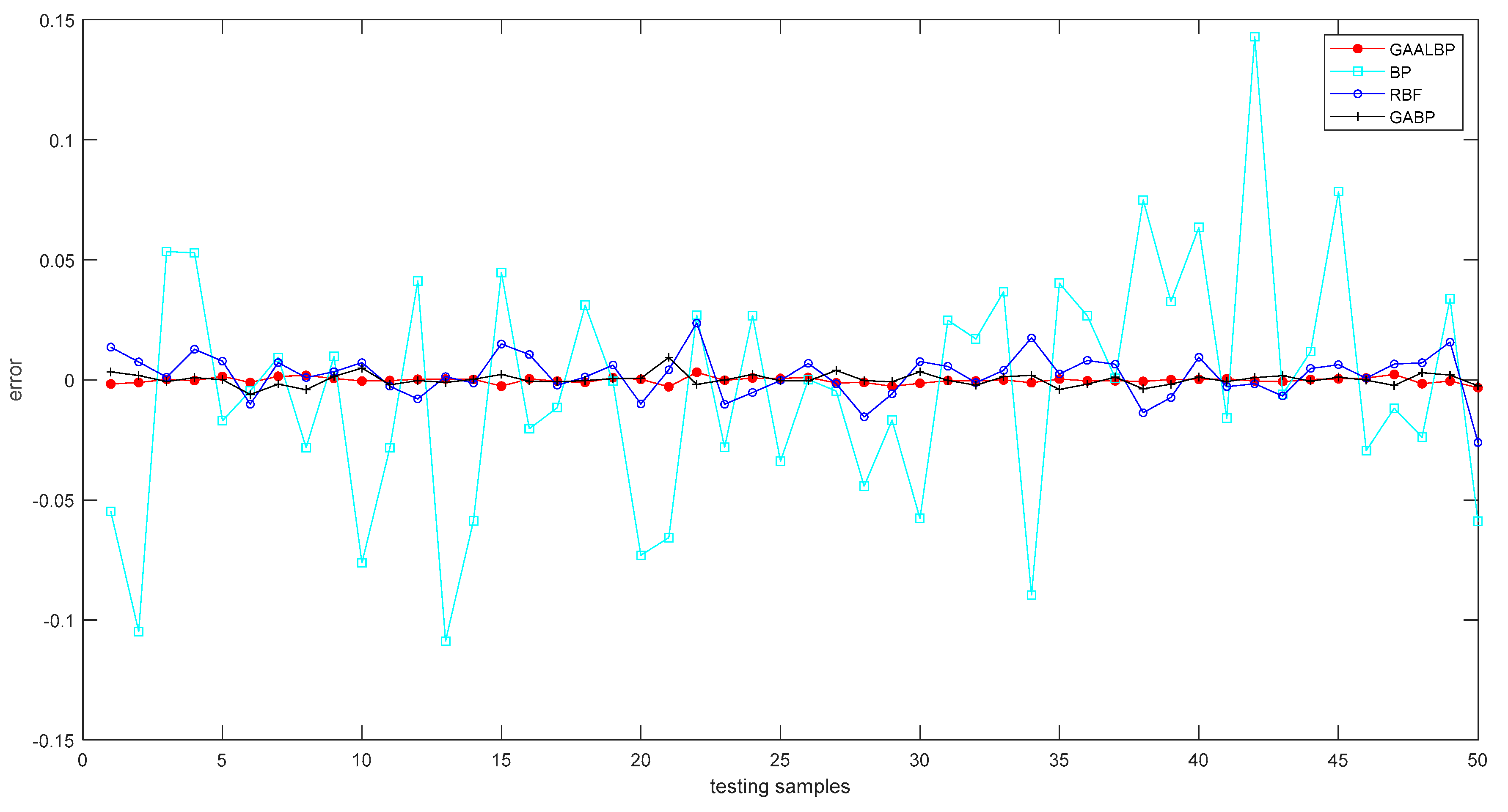
This paper proposes a surrogate model-based method for optimizing the thermal parameters of space telescopes, called SMPO. The method employs a BP neural network surrogate model based on the adaptive learning rate (called GAALBP) so as to bear a lower computational cost than the traditional thermal design approach of solving partial differential equations. Additionally, the proposed method uses a genetic algorithm (GA) to optimize the weights and thresholds of the BP network and thus improves the accuracy of the surrogate model. After the surrogate model is established, the genetic algorithm is used again to optimize the input of the network so that the output of the network approximates the target value.

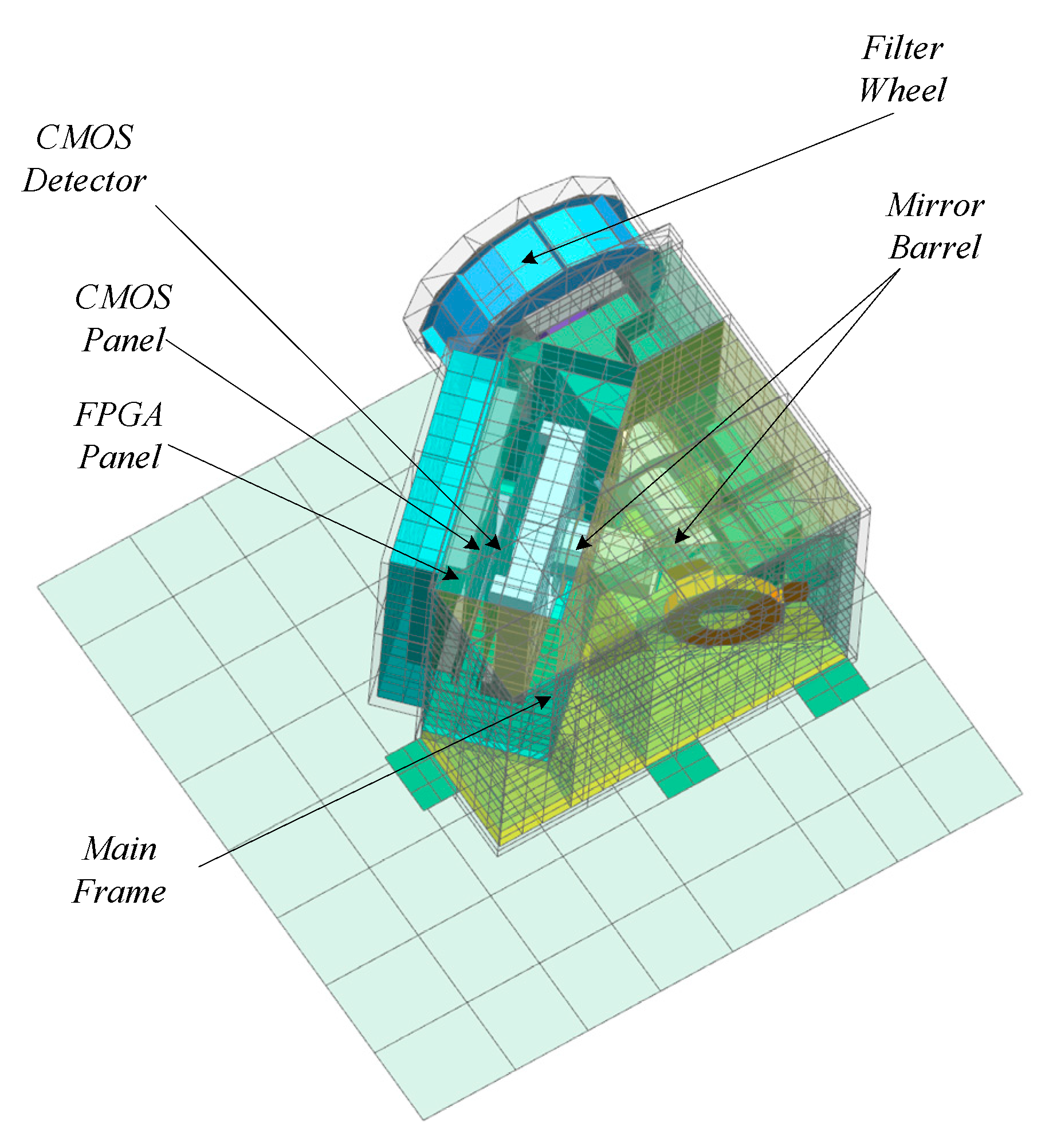
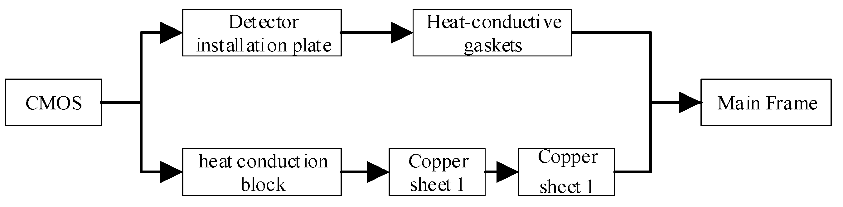
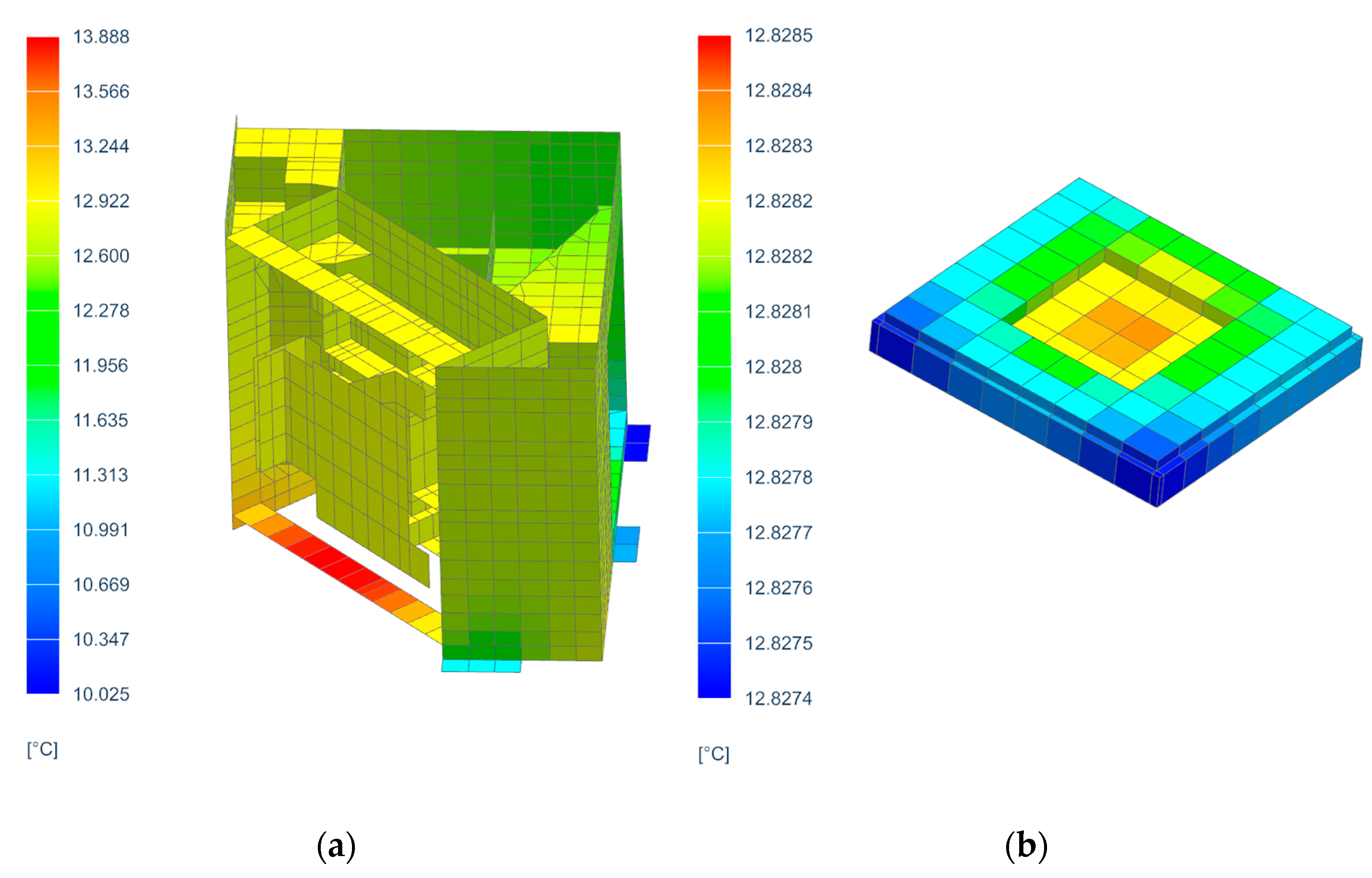
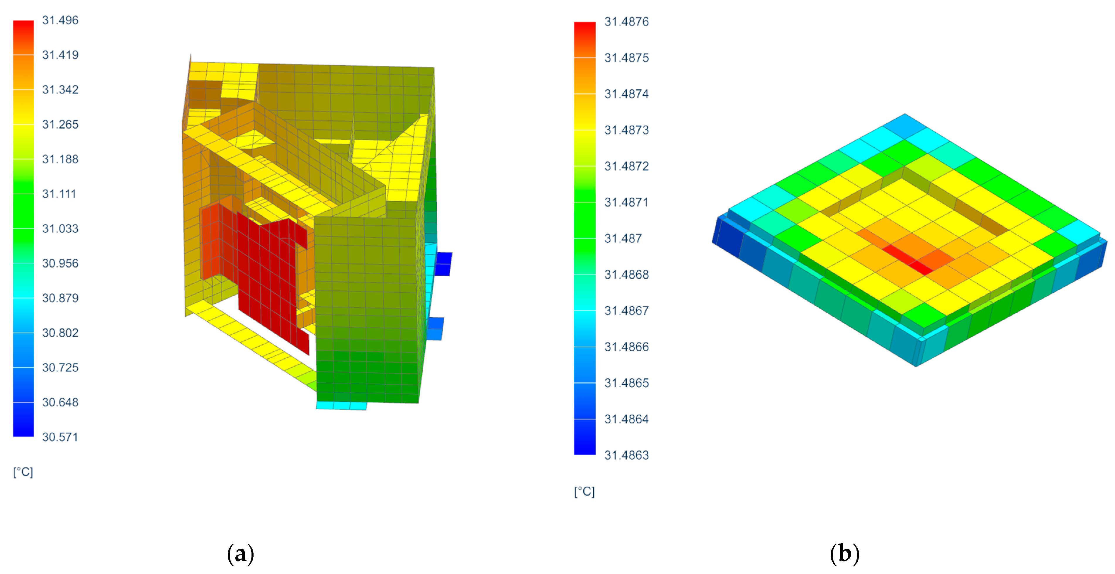
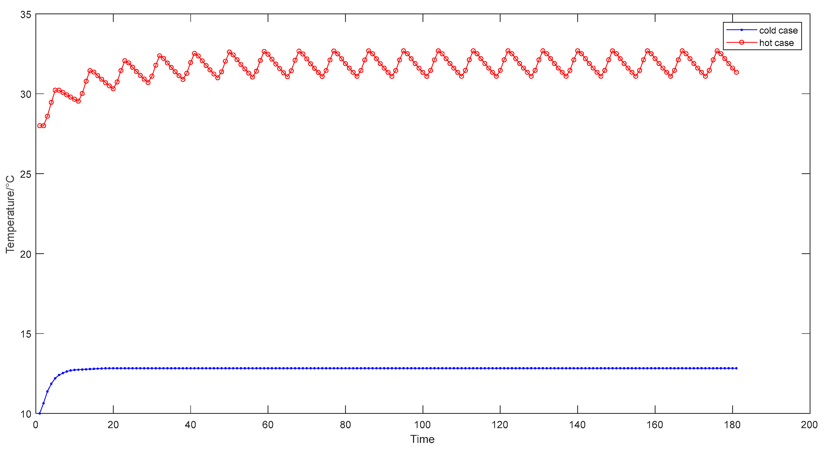
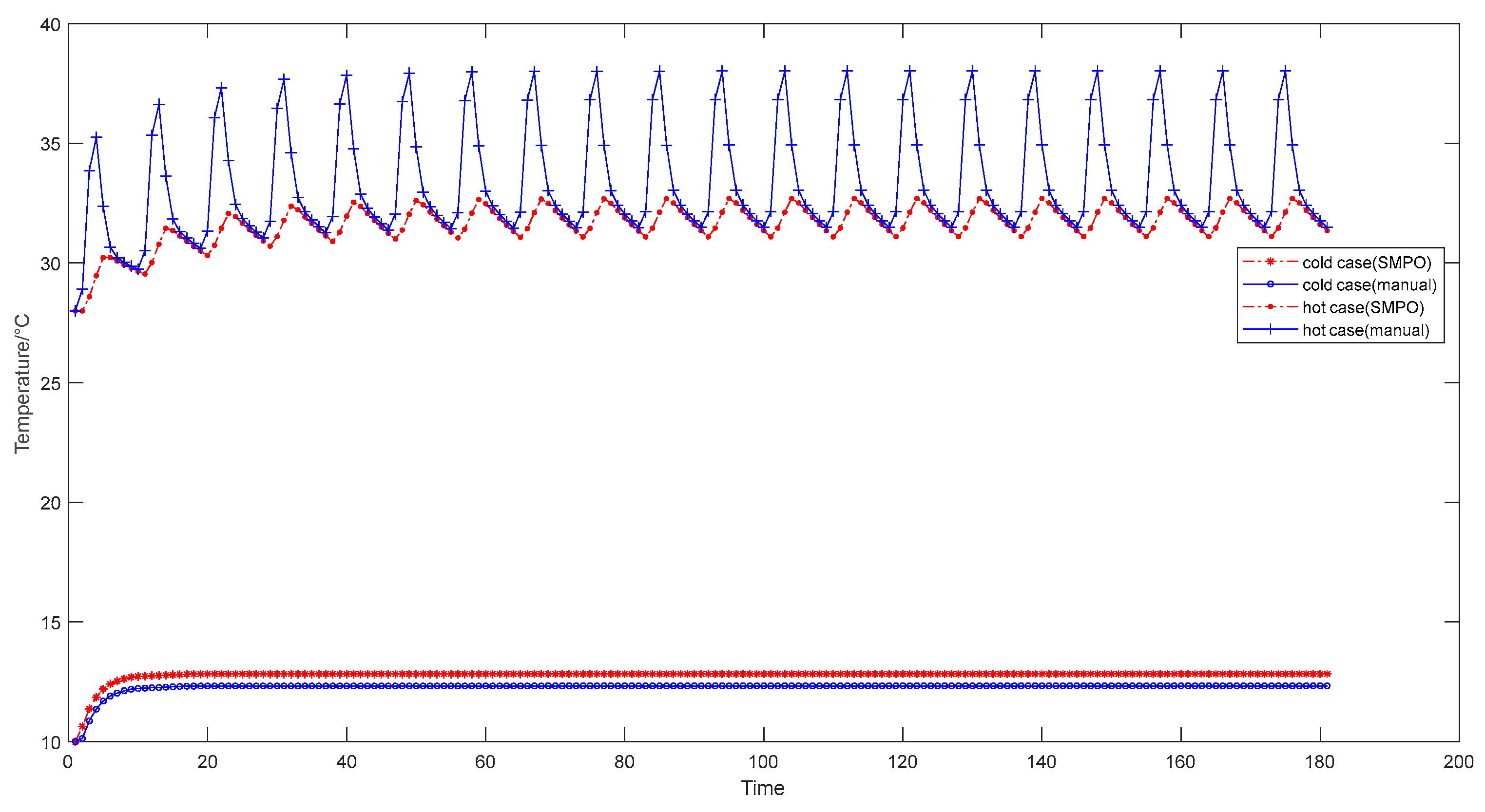
In this paper, we established a thermophysical model of a space telescope (called the ADST), selected 11 parameters of the heat dissipation path of the CMOS detector as indicators to be optimized, applied the GAALBP network surrogate model to approximate the thermophysical model of the ADST, established the mapping relationship between the 11 indicators to be optimized and the temperature of the CMOS, and used a GA to optimize indicators ensuring the output meets CMOS temperature requirements. The theoretical and simulation results reveal that SMPO proposed in the paper outperforms traditional engineer-dependent optimization, in terms of the model evaluation accuracy and higher computational efficiency.

Space telescopes are developing toward the direction of modularization, rapid launch, and short design cycles. Optimization design methods such as those similar to SMPO that can quickly realize multi-parameter intelligence and automation is of particular importance. Moreover, SMPO is an optimization framework and an optimization idea. The rapid optimization process can be transplanted into other models to achieve rapid thermal design and batch implementation. SMPO is applicable to not only the optimization of the thermal design parameters of space telescopes but also post-processing and design optimization in other fields. However, the convergence of SMPO is not particularly stable, and the SMPO optimization framework does not automate the post-processing of data, with manual data conversion still a requirement. Therefore, it remains necessary to further improve the convergence and stability of the SMPO, and to achieve full automation of SMPO.

References

- Xiong, Y.; Guo, L.; Tian, D.F. Application of Deep Reinforcement Learning to Thermal Control of Space Telescope. J. Therm. Sci. Eng. Appl. 2022, 14, 10. [Google Scholar] [CrossRef]
- Xiong, Y.; Guo, L.; Wang, H.L.; Huang, Y.; Liu, C.L. Intelligent Thermal Control Algorithm Based on Deep Deterministic Policy Gradient for Spacecraft. J. Thermophys. Heat Transf. 2020, 34, 683–695. [Google Scholar] [CrossRef]
- Xiong, Y.; Guo, L.; Yang, Y.T.; Wang, H.L. Intelligent sensitivity analysis framework based on machine learning for spacecraft thermal design. Aerosp. Sci. Technol. 2021, 118, 15. [Google Scholar] [CrossRef]
- Xiong, Y.; Guo, L.; Tian, D.F.; Zhang, Y.; Liu, C.L. Intelligent Optimization Strategy Based on Statistical Machine Learning for Spacecraft Thermal Design. IEEE Access 2020, 8, 204268–204282. [Google Scholar] [CrossRef]
- Del Rio, M.S.; Pareschi, G. Global optimization and relectivity data fitting for X-ray multilayer mirrors by means of genetic algorithms. In Proceedings of the X-ray Mirrors, Crystals, and Multilayers Conference, San Diego, CA, USA, 2–4 August 2001; pp. 88–96. [Google Scholar]
- Zhang, C.X.; Yuan, Y.; Yu, Z.Y.; Wang, F.Q.; Tan, H.P. Inversion of stellar spectral radiative properties based on multiple star catalogues. J. Cosmol. Astropart. Phys. 2018, 2018, 26. [Google Scholar] [CrossRef] [Green Version]
- Yang, X.J.; Jiao, Q.J.; Liu, X.K. Center Particle Swarm Optimization Algorithm. In Proceedings of the IEEE 3rd Information Technology, Networking, Electronic and Automation Control Conference (ITNEC), Chengdu, China, 15–17 March 2019; pp. 2084–2087. [Google Scholar]
- Yang, H.F.; Yang, Y.; Kong, D.J.; Dong, D.C.; Yang, Z.Y.; Zhang, L.H. An Improved Particle Swarm Optimization Algorithm. In Proceedings of the 9th International Conference on Natural Computation (ICNC), Shenyang, China, 23–25 July 2013; pp. 407–411. [Google Scholar]
- Stanoyevitch, A.; ACM. Homogeneous Genetic Algorithms. In Proceedings of the Annual Conference of Genetic and Evolutionary Computation Conference, London, UK, 7–11 July 2007; p. 1532. [Google Scholar]
- Laboudi, Z.; Chikhi, S. Comparison of Genetic Algorithm and Quantum Genetic Algorithm. Int. Arab J. Inf. Technol. 2012, 9, 243–249. [Google Scholar]
- Ben Salem, M.; Tomaso, L. Automatic selection for general surrogate models. Struct. Multidiscip. Optim. 2018, 58, 719–734. [Google Scholar] [CrossRef]
- Bouhlel, M.A.; Hwang, J.T.; Bartoli, N.; Lafage, R.; Morlier, J.; Martins, J. A Python surrogate modeling framework with derivatives. Adv. Eng. Softw. 2019, 135, 13. [Google Scholar] [CrossRef] [Green Version]
- Zhang, J.; Chowdhury, S.; Messac, A. An adaptive hybrid surrogate model. Struct. Multidiscip. Optim. 2012, 46, 223–238. [Google Scholar] [CrossRef]
- Vitali, R.; Haftka, R.T.; Sankar, B.V. Multi-fidelity design of stiffened composite panel with a crack. Struct. Multidiscip. Optim. 2002, 23, 347–356. [Google Scholar] [CrossRef]
- Zhang, R.X.; Zen, R.; Xing, J.F.; Arsa, D.M.S.; Saha, A.; Bressan, S. Hydrological Process Surrogate Modelling and Simulation with Neural Networks. In Proceedings of the 24th Pacific-Asia Conference on Knowledge Discovery and Data Mining (PAKDD), Electr Network, Singapore, 11–14 May 2020; pp. 449–461. [Google Scholar]
- Yan, Z.H.; Zeng, L. The BP Neural Network with MATLAB. In Proceedings of the International Conference on Electrical, Control and Automation Engineering (ECAE), Hong Kong, China, 1–2 December 2013; pp. 565–569. [Google Scholar]
- Wang, Y.; Gu, D.W.; Li, W.; Li, H.J.; Li, J. Network Intrusion Detection with Workflow Feature Definition Using BP Neural Network. In Proceedings of the 6th International Symposium on Neural Networks, Wuhan, China, 26–29 May 2009; p. 60. [Google Scholar]
- Cui, Y.Q.; Liu, H.F.; Wang, Q.L.; Zheng, Z.Q.; Wang, H.; Yue, Z.Y.; Ming, Z.Y.; Wen, M.S.; Feng, L.; Yao, M.F. Investigation on the ignition delay prediction model of multi-component surrogates based on back propagation (BP) neural network. Combust. Flame 2022, 237, 16. [Google Scholar] [CrossRef]
- Zhao, L.Y.; Gao, X.Y.; Chen, T.; Yin, W.B.; Zuo, X.; IEEE. GA-BP Neural Network Based Meta-Model Method for Computational Fluid Dynamic Approximation. In Proceedings of the IEEE 6th International Conference on Control Science and Systems Engineering (ICCSSE), Beijing, China, 17–19 July 2020; pp. 51–56. [Google Scholar]
- Hao, P.; Yuan, J.L.; Zhong, L.; IEEE. Probing modification of BP neural network learning-rate. In Proceedings of the International Conference on Machine Learning and Cybernetics, Beijing, China, 4–5 November 2002; pp. 307–309. [Google Scholar]
- Zhang, R.; Xu, Z.B.; Huang, G.B.; Wang, D.H. Global Convergence of Online BP Training with Dynamic Learning Rate. IEEE Trans. Neural Netw. Learn. Syst. 2012, 23, 330–341. [Google Scholar] [CrossRef] [PubMed]
- Whitley, D. A GENETIC ALGORITHM TUTORIAL. Stat. Comput. 1994, 4, 65–85. [Google Scholar] [CrossRef]
- Ersoy, N. Selecting the Best Normalization Technique for ROV Method: Towards a Real Life Application. Gazi Univ. J. Sci. 2021, 34, 592–609. [Google Scholar] [CrossRef]
- Kovacs, R.; Jozsa, V. Thermal analysis of the SMOG-1 PocketQube satellite. Appl. Therm. Eng. 2018, 139, 506–513. [Google Scholar] [CrossRef]
- Andras, P. Orthogonal RBF neural network approximation. Neural Process. Lett. 1999, 9, 141–151. [Google Scholar] [CrossRef]
Publisher’s Note: MDPI stays neutral with regard to jurisdictional claims in published maps and institutional affiliations. |
© 2022 by the authors. Licensee MDPI, Basel, Switzerland. This article is an open access article distributed under the terms and conditions of the Creative Commons Attribution (CC BY) license (https://creativecommons.org/licenses/by/4.0/).