State Analysis of the Water Quality in Rivers in Consideration of Diffusion Phenomenon

Abstract

The waters of rivers are not only used for consumption, industry and agriculture but have also found their way into the transport and energy generation sectors. Many disturbances introduced into the aquatic environment are of the natural variety, which are the result of “admixtures” contained in water, e.g., through contact with soil, and of man-made types, which are directly related to humanities destructive influences. In the presented examinations, the most important processes affecting the spread and transport of these pollutants are taken into account, i.e., advection and diffusion. The authors present observations on the influence of the diffusion phenomenon on river flow modelling processes. Such an approach allows for the separation of the dynamics of water flow and the dynamics of transport of the dissolved substance mass. Specifically, phenomena occurring in relation to spatial coordinates, time and variable parameter values in the proposed mathematical model were analysed. Ultimately, this research will contribute to the correct design and implementation of a complementary diffusion module as an extension to an intelligent water quality control and monitoring system. The Intelligent Analytical Computing Control System architecture under development already includes other modules such as the Intelligent Filtration and Prediction Module and, complemented by the Intelligent Diffusion Module, provides a complementary tool for monitoring river hydromorphology. Implementation of the above solution will help to improve water quality, thus preventing and eliminating the appearance of undesirable pollutants in rivers, and increase the standard of living in the current threatened environmental world.

1. Introduction

In the age of rapid change and rapid civilisational development, the terms ecology and environmental protection are becoming increasingly important. The environment influences man, and man also influences the place in which he lives, with the difference that our influence is often destructive. However, much of this inappropriate activity can be eliminated by adopting an environmentally friendly attitude. Amongst the many different factors that determine the level of civilisation is water. The requirements for water composition are continually increasing, which is why water purity tests are constantly conducted. This has resulted in the improvement and implementation of highly efficient and often unconventional manufacturing processes that protect the environment. Water is in constant motion, moving on land, in the atmosphere and in the oceans. Rivers play an important role; they form an integral part of water management and are a renewable source of fresh water. Due to the introduction of various biological and chemical substances into the environment, the quality of water has been changing [1,2]. Above all, we humans pose a very great threat to this precious resource.

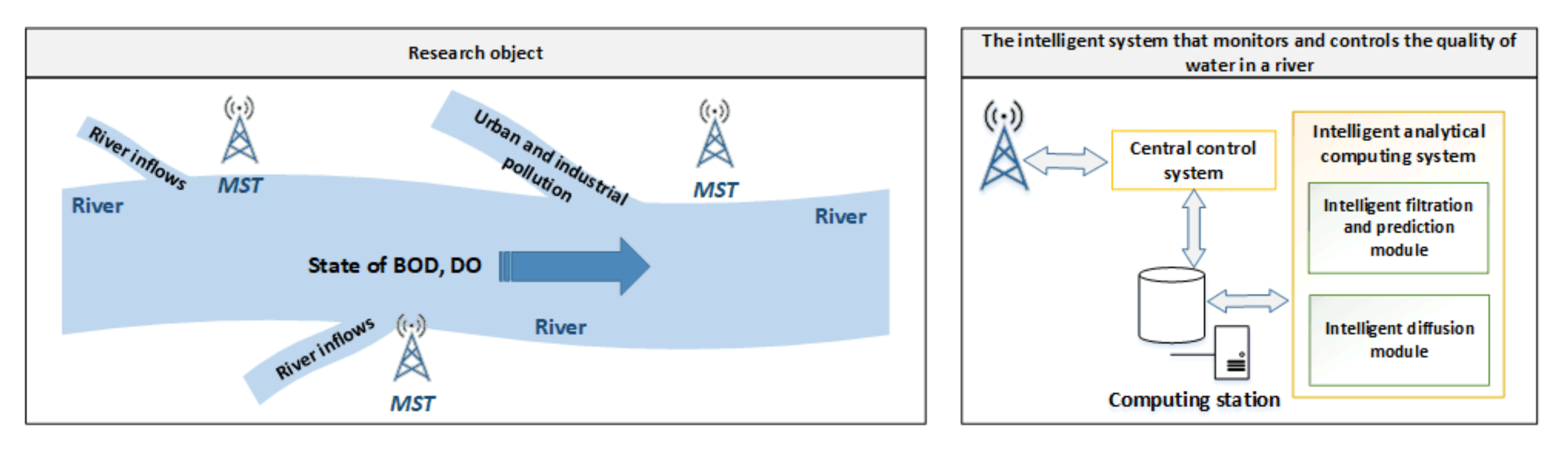
Using mathematical modelling as a tool that can be applied in various areas of research, on modern engineering solutions [3,4], the authors designed an intelligent control and monitoring system for water quality status in rivers (Figure 1). The use of the above system makes it possible to influence the improvement of water quality, thus preventing the appearance of undesirable water pollution conditions in a river, thereby augmenting the standard of living in the current threatened environmental world.

The system combines mathematical modelling and an extensively developed IT tool to monitor the state of water quality and influence its improvement when undesirable conditions arise. The intelligent monitoring and control system is the answer to the demands of Industry 5.0. Its various components, consisting of different types of sensors that monitor the state of water quality and telemetry stations that send real-time data to the intelligent module, enable the monitoring and the prevention of the spread of emerging poor water conditions. A detailed description of the system and the results of research carried out to date, in connection with the intelligent monitoring and control system, are presented in [5,6,7]. The paper [6] presents an approach which employs ANN (Artificial Neural Networks) for the real-time monitoring and control of water quality status. The paper [5] presents a spatio-temporal method for analysing the state of river pollution, in the context of application in modern control and measurement systems, for predicting changes. On the other hand, the paper [7] presents an adaptive algorithm to determine the value of the filter amplification factor, which allows for the avoidance of inconveniences, resulting from the need to estimate the characteristics of signals affecting the object under investigation. In this work, the mathematical models used did not make use of the phenomenon of diffusion which, under certain conditions of the river environment, significantly weakened the accuracy of the monitoring process.

Theoretical and experimental studies of diffusion in liquids are discussed by many authors in various scientific publications [8,9,10]. The paper [11] focuses on discussing the principles, applications and advances in diffusion, thermal diffusion and thermal conductivity in liquid systems. The presented experimental methods, for studying diffusion processes in liquids, systematise the theoretical interpretation of diffusion coefficients. In explaining the control of the specific gravity of an air–water mixture, the authors [12] use the partial differential equation of convective diffusion at a constant state. The equation being considered contains diffusion and convection coefficients which are treated as control variables in the process of minimising the error evaluation function between the observed specific gravity and the solution of the control equation. In the study, discussed in the literature item [13], the one-dimensional advection-diffusion equation with variable coefficients, was solved for three dispersion problems: (a) dissolved substance dispersion in steady flow through a heterogeneous medium, (b) time-dependent dissolved substance dispersion in homogeneous flow, through a homogeneous medium, and (c) dissolved substance dispersion along time-dependent flow, through a heterogeneous medium. The new independent variables are introduced through separate transformations, in terms of which the advection-diffusion equation in each problem is reduced to an equation with constant coefficients. By considering contaminants that are chemically inert and flow passively with the carrier fluid undergoing diffusion, the authors investigated the diffusion behaviour of a passive contaminant in a progressive wave field with strong turbulence using analytical methods [14]. The focus is on nonlinear interactions between stochastic diffusion and deterministic wave-induced oscillatory advection. The scope of the study was limited to cases where there is a small parameter $\delta$ between advective and diffusive displacements, which allowed the disturbance analysis to be conducted. The study [15,16] evaluated different definitions of the Péclet number for their ability to determine the relative importance of transport by advection and transport by diffusion, in low-permeability environments. It was identified that when deciding not to consider advection in low-permeability environments, the Péclet number, including the porosity available for diffusion, should be used instead of the effective porosity value.

In this paper, the authors present considerations on the influence of diffusion, in the process of modelling flow phenomena, which constitutes another intelligent module in the developed system for monitoring and controlling water quality status. Many elements introduced into the aquatic environment are passive and conservative; therefore, the most important processes influencing the spread and transport of these pollutants, i.e., advection and diffusion, are considered in the presented numerical experiments. This allows one to separate the dynamics of water flow and the dynamics of the transport of the dissolved substance mass.

2. Materials and Methods

2.1. Water Quality Indicators

Water is a fundamental element of any national economy. The analyses of changes in water pollution indicators, namely Biochemical Oxygen Demand (BOD) and Dissolved Oxygen (DO) levels, are interesting and complex scientific problems [17,18]. Mathematical modelling plays a major role here. Organic and inorganic substances contribute to surface water pollution. The most important components affecting water quality status are Total Organic Carbon (TOC) [19], Chemical Oxygen Demand (COD) and BOD. BOD${}_5$ is a standard five-day test at 20 ${}^{\circ }$C to determine the assimilable fraction of a mixture of organic substances. Complete oxidation of organic compounds, under the given conditions, occurs within 28 days. The BOD${}_k$ or BOD${}_c$ indicators correspond to the final and total oxygen consumption. Biochemical oxygen demand BOD${}_5$ is a conventional indicator of organic pollution, while BOD is a representation of the decomposition processes of organic compounds in water. The process of BOD changes are assessed by measuring dissolved oxygen consumption. This process is very complex and depends on many factors including: oxygen content, type of organic compounds existing in the water, microorganisms and environmental factors [20,21,22,23].

The above processes can be described by a first-order differential equation. It is assumed that the rate of decomposition of organic substances is proportional to the concentration of the remaining nonoxidised substances. The BOD changes by a well-defined value over a specific time interval:

$$\frac{d{x}_1}{dt}=-k_1{x}_1$$

(1)

where $x_1$—BOD value [mg/L] over time t and $k_1$—first order reaction rate constant. At the same time, as the substrate concentration decreases further, the decomposition rate changes. Assuming that the initial value of BOD at time $t_0$ is $x_0$ and decreases to $x_1$ after time t, the analytical solution of Equation (1) takes the form:

$$ln\frac{x_1}{x_0}=-k_{1}t,x_1=x_0{e}^{-k_{1}t}$$

(2)

Because the rate of the BOD process is strongly influenced by temperature, the BOD process is accelerated with increasing temperature. If the optimum value is exceeded, the process is inhibited or even disappears. The relationships shown above are valid only for values obtained at the same temperatures:

$$k_1=k_{20}{\theta }^{\left(t-20\right)}$$

(3)

where the $\theta$—temperature-dependent thermal coefficient. At temperatures ${〈20,30〉}^{\circ }$C, the thermal coefficient is 1.056, while at interval ${〈4,20〉}^{\circ }$C the coefficient takes on a value of 1.135. Theoretically, the $k_1$-value should be constant and is dependent on the concentration and type of organic matter, the type and activity of the microorganisms, and the temperature. Two phases can be distinguished in the BOD test: fast and slow. The first phase is characterised by a high $k_1$-value, where fast decomposition and synthesis of biomass occurs, with the rapid consumption of dissolved oxygen in the water. In the second phase, the coefficient $k_1$ takes on small values. In this phase, slow endogenous respiration processes take place. The values of $k_1$ can take values between approximately $〈0.01,0.30〉{\mathrm{d}}^{-1}$(${\mathrm{d}}^{-1}$ —per day). At temperature 20 ${}^{\circ }$C, the average $k_1$ values are: $〈0.04,0.08〉{\mathrm{d}}^{-1}$ for low-pollution rivers, $〈0.06,0.10〉{\mathrm{d}}^{-1}$ for low-pollution rivers, $〈0.12,0.22〉{\mathrm{d}}^{-1}$ for partially treated wastewater, $〈0.15,0.30〉{\mathrm{d}}^{-1}$ for raw wastewater. The $k_1$ value depends on the activity of the microorganisms and decreases as the activity decreases. The increase in $k_1$ with temperature is represented by relation (3).

Dissolved oxygen is one of the most important indicators of water quality: it influences the chemical and biochemical processes that occur in water. DO is an important indicator for the living organisms that make up a river ecosystem [24,25,26]. Aerobic processes occurring in natural waters are essential for reducing pollution in water. These processes take place in the presence of oxygen, and the lack of oxygen in the water leads to anaerobic processes in which odorous substances are produced. The solubility of oxygen in water depends on the temperature, as the temperature increases the dissolved oxygen decreases. Another factor in the reduction of dissolved oxygen is an increase in salinity. Furthermore, the drop in pressure causes the dissolved oxygen to decrease, which is why the solubility of oxygen is usually quoted at a pressure of one atmosphere (101,325 Pa). Oxygen deficiency is the loss of dissolved oxygen in water. This is the difference between the maximum and current oxygen concentration. In other words, the deficit is the amount of oxygen that must be introduced into the water to achieve maximum saturation. The rate of water deoxygenation is directly proportional to the BOD, which is represented by the following relation:

$$\frac{dD}{dt}=k_1{x}_1$$

(4)

where $\frac{dD}{dt}$—rate of change of oxygen deficit [mg/L], $k_1$—BOD, and $x_1$—BOD over time t. In order to take into account the BOD value of the water at the wastewater discharge point, denoted as $x_{10}$, the relation (2) must be inserted into relation (4):

$$x_1=x_{10}{e}^{-k_{1}t}$$

(5)

in which $x_{10}$ is the BOD concentration at time $t_0$. From the above, the following relationship is obtained:

$$\frac{dD}{dt}=k_1{x}_{10}{e}^{\left(-k_{1}t\right)}$$

(6)

In parallel with the deoxygenation of the water, oxygenation (re-aeration) occurs as a result of constant contact between the water surface and atmospheric air. Oxygen uptake by the water surface takes place at a rate proportional to the actual oxygen deficit, according to the relationship:

$$\frac{dD}{dt}=-k_{2}D$$

(7)

where $k_2$—oxygen uptake (re-aeration) rate coefficient $\left[{\mathrm{d}}^{-1}\right]$. The uptake re-aeration coefficient $k_2$ depends on the water temperature and flow characteristics of the river, such as: flow rate and river bed depth. The influence of temperature on the value of the re-aeration coefficient $k_2$ is shown in the relation:

$$k_{2\left(T\right)}=k_{2\left({20}^{\circ }C\right)}{\theta }^{\left(t-20{}^{\circ }\mathrm{C}\right)}$$

(8)

where the $\theta$ thermal coefficient is equal to 1.047. The value of the $k_2$ coefficient is lower in deep and slow-flowing waters than in shallow and fast-flowing waters. The basis for determining the $k_2$ coefficient is the analysis of the watercourse profile:

$$k_2\left(20{}^{\circ }\mathrm{C}\right)=2.833\left(V/H^{3/\phantom{2}2}\right)$$

(9)

where V—average flow velocity of the watercourse [m/s]; H—average depth of the watercourse [m]; and 2.833—correction factor related to roughness changes of the bottom surface of the watercourse.

2.2. Streeter–Phelps Mathematical River Model

The widely used Streeter–Phelps model is used to predict oxygen demand, following the introduction of pollutants into a river. This makes it possible to determine the oxygen concentration in successive sections of a polluted river. The essence of the model is an equation of the oxygen balance between two competing processes: the uptake of oxygen from the water, associated with the removal of organic carbon compounds, and the supply of oxygen from the atmosphere to the water through re-aeration. The Streeter–Phelps model is helpful for predicting the changes that occur in a polluted river [27,28,29]. It is assumed that the equations describe the reaction, under conditions of ideal and continuous mixing (the so-called continuous mixing chemical reactor). When considering changes in rivers, this situation refers to a certain stretch of water in the river. The effect of this approach is to obtain connected “reactors” for which the state of pollution is monitored, i.e., to divide the river into small sections. Otherwise, the river should be divided into sections corresponding to changes in flow or pollutant inflows. Each section should be treated as an individual case of the model considered [5,6,7]. Based on the Streeter–Phelps formulation, the process of BOD and DO changes can be modelled by differential equations:

$$\frac{d{x}_1}{dt}=-k_1{x}_1,x_1\left(t_0\right)=x_{10}$$

(10)

where $x_1\left[\mathrm{mg}/\mathrm{L}\right]$—BOD, $t\left[\mathrm{day}\right]$—time, and $k_1\left[{\mathrm{d}}^{-1}\right]$—reaction rate coefficient. By contrast, the change in DO level is:

$$\frac{d{x}_{2N}}{dt}=-k_2{x}_1+k_3\left(x_{2N}-x_2\right)+a$$

(11)

where $x_{2N}\left[\mathrm{mg}/\mathrm{L}\right]$—DO concentration, $k_2\left[{\mathrm{d}}^{-1}\right]$—rate coefficient for the influence of BOD on DO, $k_3\left[{\mathrm{d}}^{-1}\right]$—rate coefficient for the uptake of oxygen from the atmosphere, and $a\left[\mathrm{mg}/\mathrm{L}·\mathrm{d}\right]$—intensity of oxygen supply. Denoting $x_2$ as DO deficit understood as:

$$x_2=x_{2N}-x_{2s}$$

(12)

The change in DO deficit over time can be described by the relationship:

$$\frac{d{x}_2}{dt}=-k_2{x}_1-k_3{x}_2+a,x_2\left(t_0\right)=x_{20}$$

(13)

Using vector notation, Equations (10) and (13) take the form:

$$\frac{dx}{dt}=Ax+Bw,x_0\left(t_0\right)=x_0$$

(14)

where $A=\left[\begin{array}{cccc}-k_1& 0;& -k_2& -k_3\end{array}\right]$—state matrix, x—vector $x=col\left[x_1{x}_2\right]$, B—control matrix, and w—external excitation and control vector. Equation (14) is the starting point for considering the mathematical modelling of a river without taking into account the phenomenon of diffusion. The model is presented as a continuously stirred reservoir. The above considerations apply to a section of river of small length. For large sections, the outflow from one reservoir is the inflow of another. The result is a division of the river into many fragments interpreted individually. A detailed description of the considerations has been included in previous works [5,6,7].

2.3. River Model Described by a Partial Differential Equation of Hyperbolic Type

When considering a state vector whose coordinates are influenced by river length and time, the Streeter–Phelps equations transform to first-order hyperbolic differential equations once mass balance is taken into account [30]. These equations include a description of a part of the river called a section, e.g., for the i-th section, the equations take the form:

$$\frac{\partial x_i}{\partial t}+V\frac{\partial x_i}{\partial z}=A{x}_i+Bw$$

(15)

where $x_i$—state vector, $t\left[\mathrm{day}\right]$—time, z—length, A—state matrix, $V=diag\left(v,v\right)$—diagonal matrix with water flow velocities v, $B=diag\left(1,1\right)$—interference interaction matrix, and w—interference vector. The diagonality of the flow velocity matrix V reflects the serial character of objects of this type in which the state vector “travels” only in one direction with the same velocity. The boundary conditions, included in the model, are described by a boundary condition concerning the beginning of the considered section in the time domain:

$$x_i(0,t)=M_i{x}_{i-1}(1,t)+w_{bi}\left(t\right)+R_{bi}{u}_{bi}\left(t\right)$$

(16)

where $M_i$ is a matrix defining the boundary links between individual river sections, the $w_{bi}$ vector represents the disturbance of the boundary values, and control $u_{bi}$ only affects the coordinate of the state vector $x_2$ and is located at the beginning of the river section. The second condition is the initial condition, which applies to the entire length of the section at time $t=t_0$:

$$x_i(z,t_0)=x_{i0}\left(z\right),i=1,\dots ,N$$

(17)

The first-order hyperbolic partial differential Equation (15) represents a general approach to the river modelling, in contrast to the equations described by the Streeter–Phelps model ((10), (13) and (14)). By having a velocity matrix whose values depend on the length of the river, we do not generalise the average velocity along the length of the river but factor in the natural variations in the velocity parameter. In further considerations of the mathematical modelling of rivers, a constant value was assumed for the velocity along a given section of the river.

2.4. Mathematical Model of a River including the Phenomenon of Diffusion

The mathematical modelling of phenomena occurring in the aquatic environment makes it necessary to analyse all the factors affecting water quality. The phenomenon of diffusion is an important factor influencing water quality. Diffusion is examined considering the spatial conditions such as length, width and depth of a river. Based on the above considerations and the Gauss–Ostrogradsky theorem, the phenomenon of diffusion can be described as follows:

$$\frac{\partial x}{\partial t}-div\left(Dgradx\right)+\delta =0$$

(18)

where x—state vector dependent on river length and time, D—diffusion coefficient in the isotopic medium, and $\delta$—intensity of generation or disappearance of the transferred agent. Disregarding the velocity of water flow and taking the diffusion value as a constant, we obtain an equation of the form:

$$\frac{\partial x}{\partial t}-\frac{\partial }{\partial z}-\left(D\frac{\partial x}{\partial z}\right)+\delta =0$$

(19)

Taking into account the self-cleaning process of the river, Equation (19) is extended by an additional factor:

$$\frac{\partial x}{\partial t}-\frac{\partial }{\partial z}-\left(D\frac{\partial x}{\partial z}\right)+Ax+\delta =0$$

(20)

where $A=\left[\begin{array}{cccc}-k_1& 0;& -k_2& -k_3\end{array}\right]$ is a state matrix in which the $k_i=1,\dots ,N$ coefficients determine the rate of response of the state variables. Considering a state vector that depends on time, length and additionally on the width and depth of the river, Equation (20) has the form:

$$\frac{\partial x}{\partial t}-\left(D\frac{{\partial }^{2}x}{\partial z_1^2}+D\frac{{\partial }^{2}x}{\partial z_2^2}+D\frac{{\partial }^{2}x}{\partial z_3^2}\right)+Ax+\delta =0$$

(21)

where $z_1$, $z_2$, and $z_3$—spatial coordinates for length, width and depth, respectively. Assuming that a change in diffusion along the spatial variable, with that being the water depth, is negligible in relation to the width and length of the water body, this value can be ignored, while taking into account its flow velocity:

$$\frac{\partial x}{\partial t}-\left(D\frac{{\partial }^{2}x}{\partial z_1^2}+D\frac{{\partial }^{2}x}{\partial z_2^2}\right)+V\frac{\partial x}{\partial z_1}+Ax+\delta =0$$

(22)

where $V=diag\left(v,v\right)$—diagonal matrix representing the flow velocity over a given length $z_1$. The solution of the above equations is possible with known boundary conditions which take the following form:

$$x\left(z_1,t_0\right)=f_{p1}\left(z_1\right)$$

(23)

$$x\left(z_2,t_0\right)=f_{p2}\left(z_2\right)$$

(24)

$$x\left(0,t\right)=f_b\left(t\right)$$

(25)

where the functions $f_{p1}$, $f_{p2}$, and $f_b$ are known for the corresponding coordinates. Ensuring the compatibility and stability of the solution requires the adoption of an appropriate discretization step factor. In order to determine the $dt$ value in conjunction with $dz$, the Courant diffusion number rule is as follows:

$$dt\le \frac{d{z}^2}{2D}$$

(26)

where D—diffusion coefficient, $dt$, and $dz$—distances between nodes. The Courant number describes a mathematical condition, for the convergence of mathematical methods, for solving hyperbolic partial differential equations. It stipulates that the length of the time step must not exceed a certain limit value; otherwise, the method loses stability. This relationship is important when testing with diffusion. Solving the advective–diffusion transport equation is difficult because the advection part is hyperbolic and the diffusion part is parabolic. The criterion for the participation of both parts in the transfer of medium is the Péclet number, which for a grid of nodes distant from each other by dx is determined as follows: $P=udx/D$, where u—average stream velocity, D—diffusion coefficient, $P=\infty$ for advectional transfer only, when $D=0,P=0$ for diffusion-only transfer, when $u=0$. However, physical oscillations may occur due to numerical dispersion. This problem arises as the Péclet number increases.

3. Results and Discussion

The results of simulation studies for models that do not take into account the diffusion phenomenon are described in [5,6,7]. The incentive for the experimental part of this paper is the attempt to test, in the form of simulation studies, the extended mathematical model which has been significantly extended in relation to the previously used simplified mathematical models of the river. The adopted experimental strategy includes sets of changing hydrological and biological parameters of the river, such as the velocity of the flow of water masses, the intensity of diffusion phenomena and the biological oxygen demand correlated with them. In this way, a comprehensive overview of the variability of the individual coordinates of the state of the process occurring in the river was created, in order to obtain an objective assessment of the accuracy of the monitoring of the ecological state of the river, which changes under their influence. These results are the starting point for the construction of an intelligent control module for the treatment process, taking diffusion under consideration. In view of the assumptions thus made based on the mathematical model of a polluted river described by Equations (10) and (13), a number of simulation studies were conducted, taking into account that measurements are made along the characteristics of free-flowing water. The mathematical model was verified for a legitimate subject, the Wislok river, covering the area of southeastern Poland. Field research was conducted on the local Wislok river, which is a hydrological object of significant importance for the Podkarpackie Province. The pollution load of the Wislok river depends on the level of development and industrialisation of individual fragments of its riverbed. Four measurement points were selected to reflect the nature of its flow in a specific way. The places where measurements were carried out are: Zarnowa (21.818889 E, 49.875556 N), Lutoryz (21.9093209 E, 49.9666064 N), Rzeszow (22.0115789 E, 50.0086266 N), and Smolarzyny (22.2924051 E, 50.1256537 N). In addition, selected measurement points are associated with the physical realisation of an intelligent monitoring and control system, using data transmission telemetry. Figure 2 illustrates the cross-sections of the riverbed, including the velocities that occur at given river latitudes.

The research presented in this paper, on the mathematical model of the river taking into account the diffusion phenomenon, is based on Equation (22) and is carried out only for the BOD coefficient. Consideration of the diffusion phenomenon is addressed, encompassing two spatial coordinates, which are time and the length of the river section. The simulation results are described in a two-dimensional area z, t for different values of D, V, and A. A first interpretation of the problem is to consider the diffusion coefficient, assuming that the values $V=0$ and $A=0$. 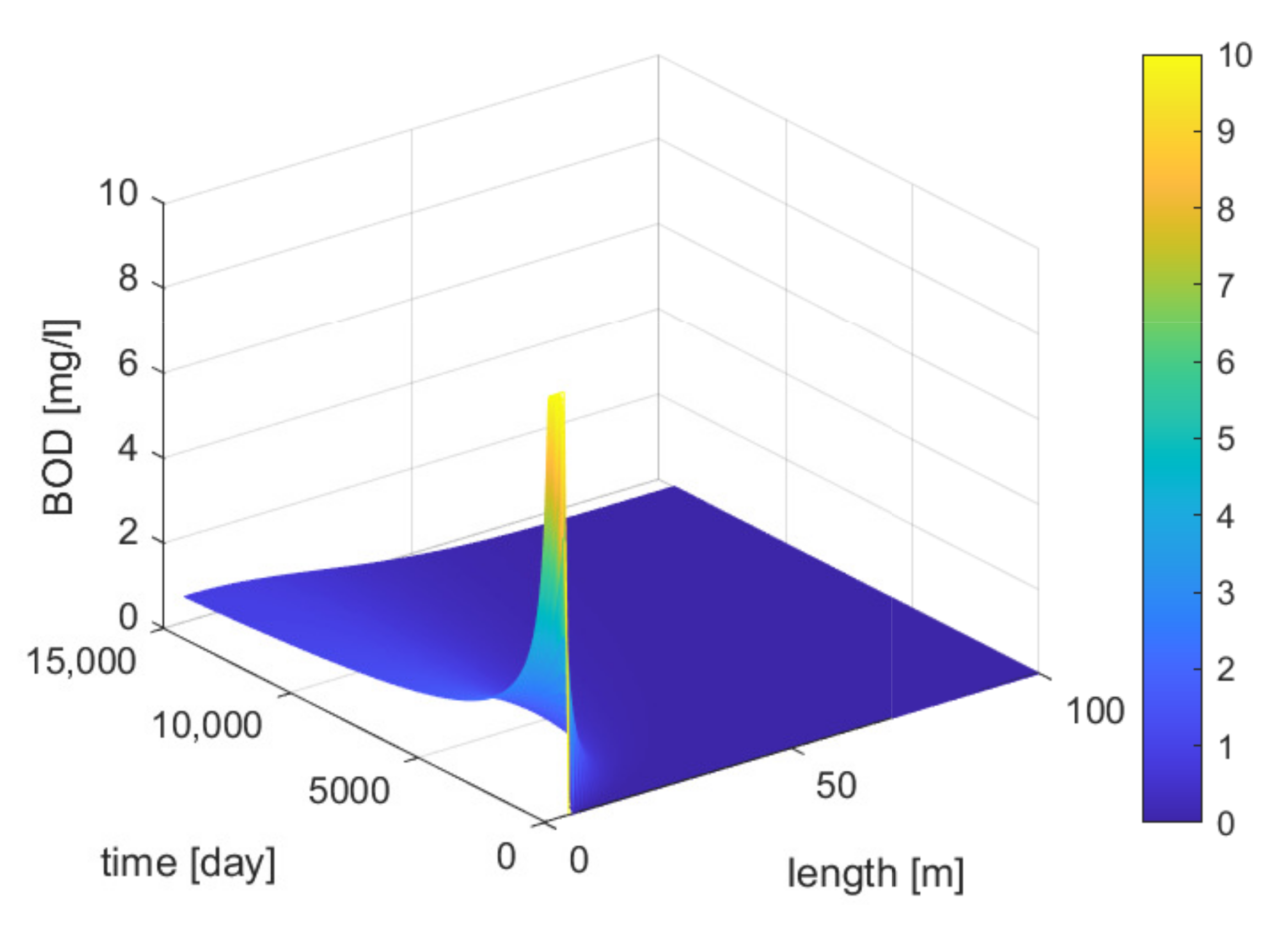The results obtained are shown in Figure 3 and

Table 1. Initial values used in the studies.

$\mathit{BOD}\left[\mathbf{mg}/\mathbf{L}\right]$	A	$\mathit{D}\left[{\mathbf{m}}^2/\mathbf{h}\right]$	$\mathit{V}\left[\mathbf{m}/\mathbf{h}\right]$	$\mathit{dz}\left[\mathbf{m}\right]$	$\mathit{dt}\left[\mathbf{h}\right]$
10	0	$3600\times$ 5 × 10${}^{-9}$	0	0.001	0.0014

summarises the initial values used in the experiments.

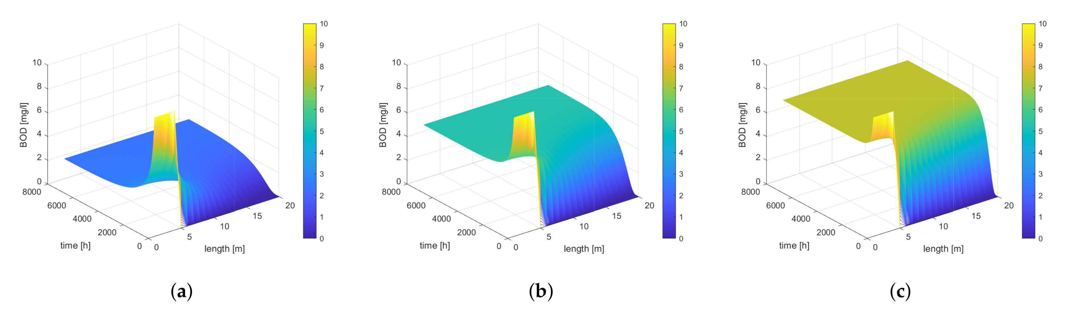
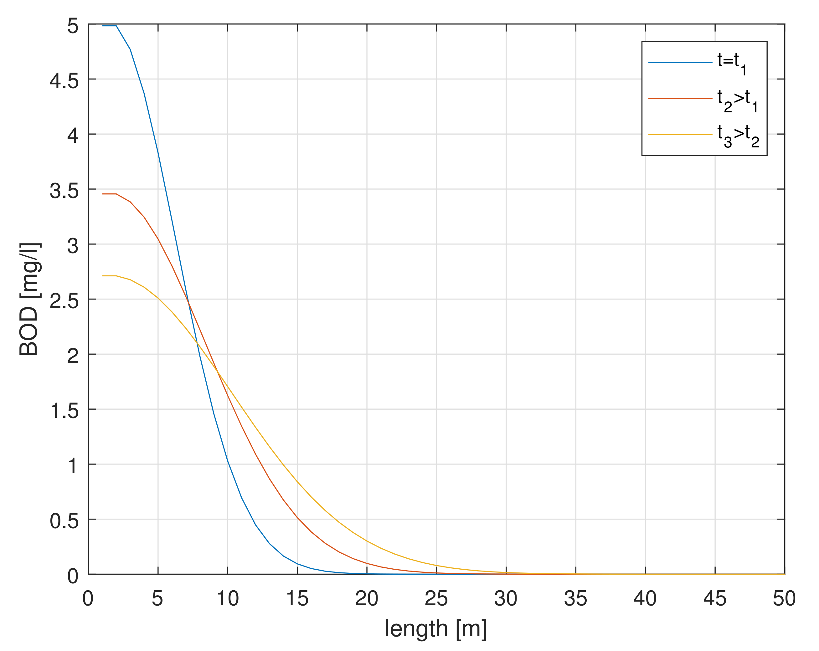
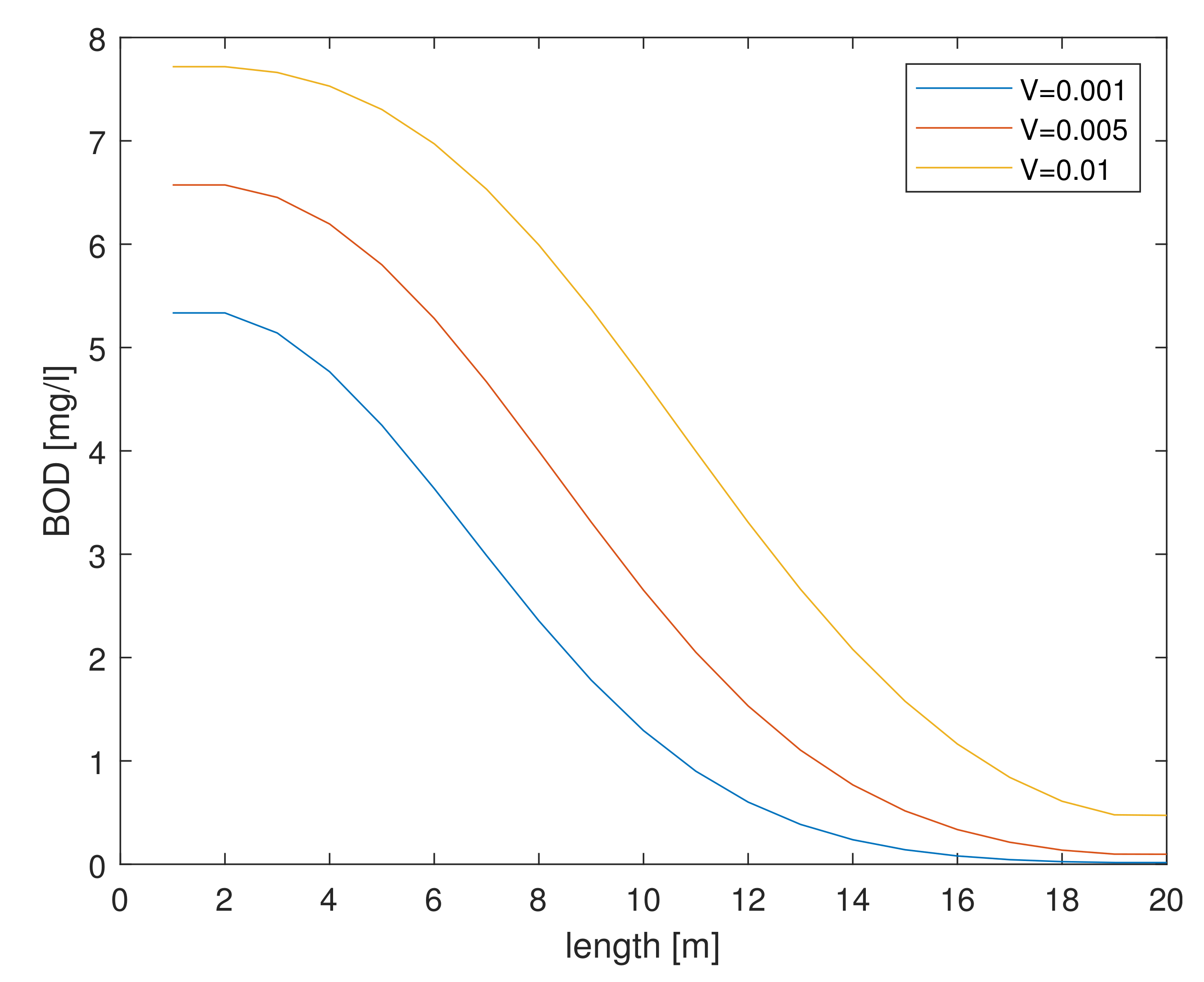
Analysing Figure 3, we can observe the appearance of pollution at the beginning of the river section under consideration. The BOD concentration decreases in the long term, which is caused by the spreading of the pollution centre. The consequence is the distribution of the concentration of pollution over a certain time and space. Here, we can see the influence of diffusion, where, after a certain period of observation, a decrease in its concentration and distribution can be seen. At different lengths, at different moments in time, the BOD concentration takes on a correspondingly different value, as demonstrated in Figure 4. Depending on the time moment, at a given river length position, BOD concentration values vary. Respectively, at the moment of, e.g., $t=t_1$, $t=t_2$, $t=t_3$ the BOD value is within the limits of 5, 3.5 and 2.7 [mg/L].

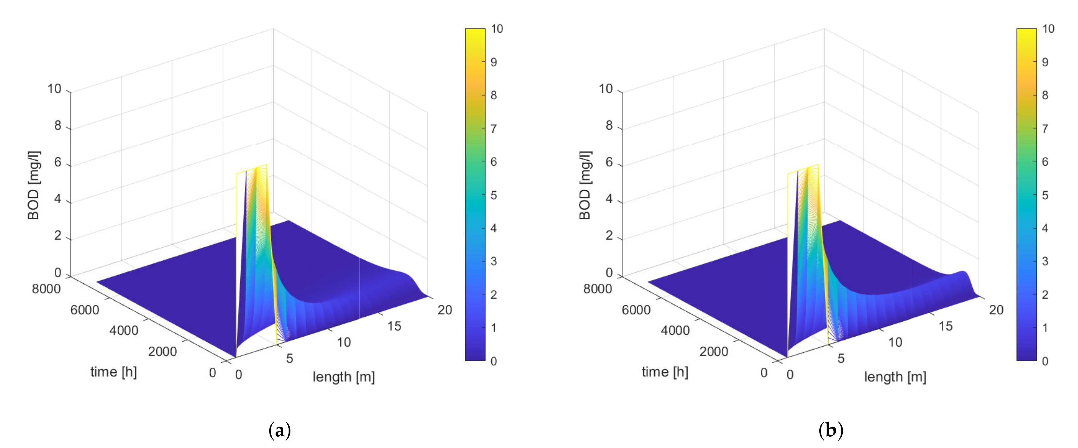
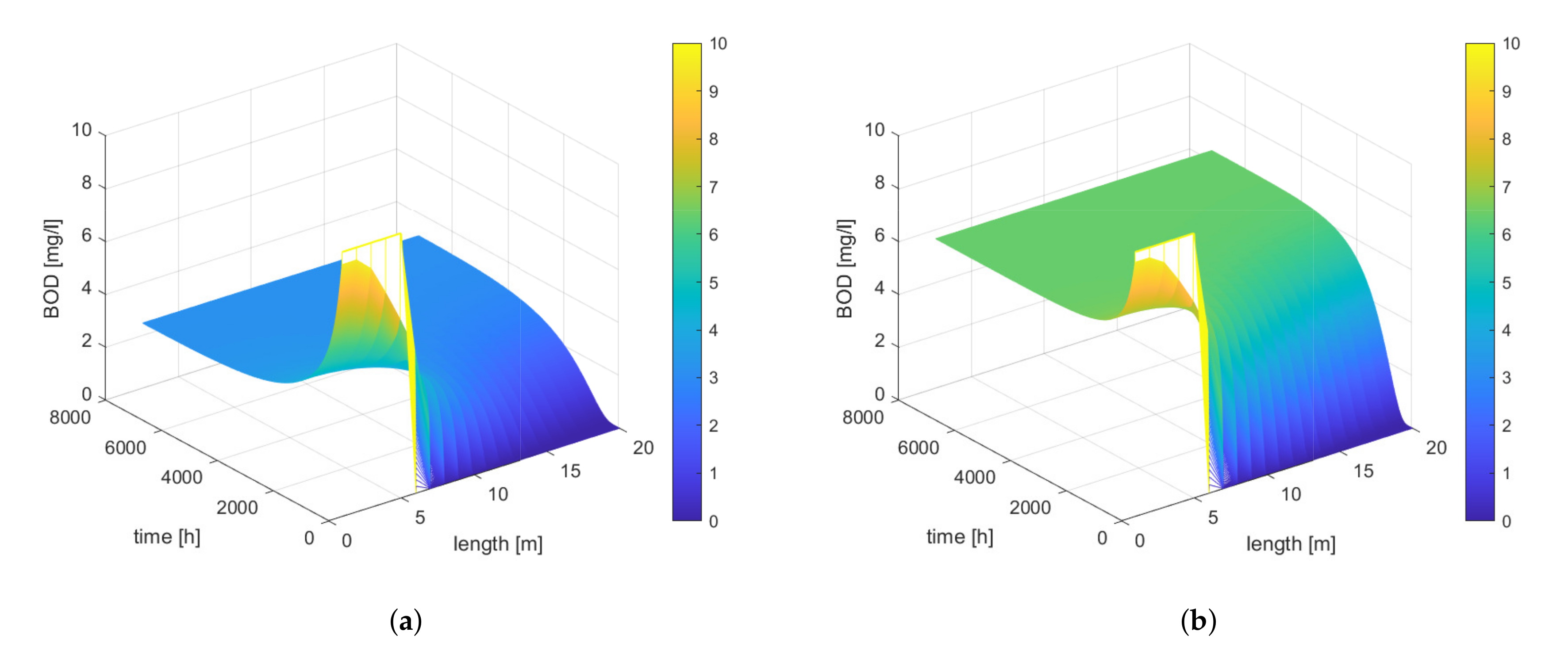
Further consideration of the effect of diffusion, on the self-cleaning process, is to consider the situation when the inflowing water on the river banks is clean. This causes pollutants to be “entrained” by the river and to decompose along its entire length. Taking into account the phenomenon of diffusion at different river speeds, the spread of pollutants along the same stretch of river is different. The results of this process model, shown in Figure 5 and

Table 2. Values used in experiments.

Value	Figure 5a	Figure 5b	Figure 6a	Figure 6b
$BOD\left[\mathrm{mg}/\mathrm{L}\right]$	10	10	10	10
A	0.2	0.2	0	0.2
$D\left[{\mathrm{m}}^2/\mathrm{h}\right]$	3600 × 5 × 10${}^{-9}$	3600 × 5 × 10${}^{-9}$	0	0
$V\left[\mathrm{m}/\mathrm{h}\right]$	0.005	0.01	0.005	0.005
$dz\left[\mathrm{m}\right]$	0.001	0.001	0.001	0.001
$dt\left[\mathrm{h}\right]$	0.0069	0.0069	0.0014	0.0014

, summarise the values used in the experiments. At the initial moment, the value of the pollution was relatively high, but as time and length change, the pollution decreases and changes in length and time.

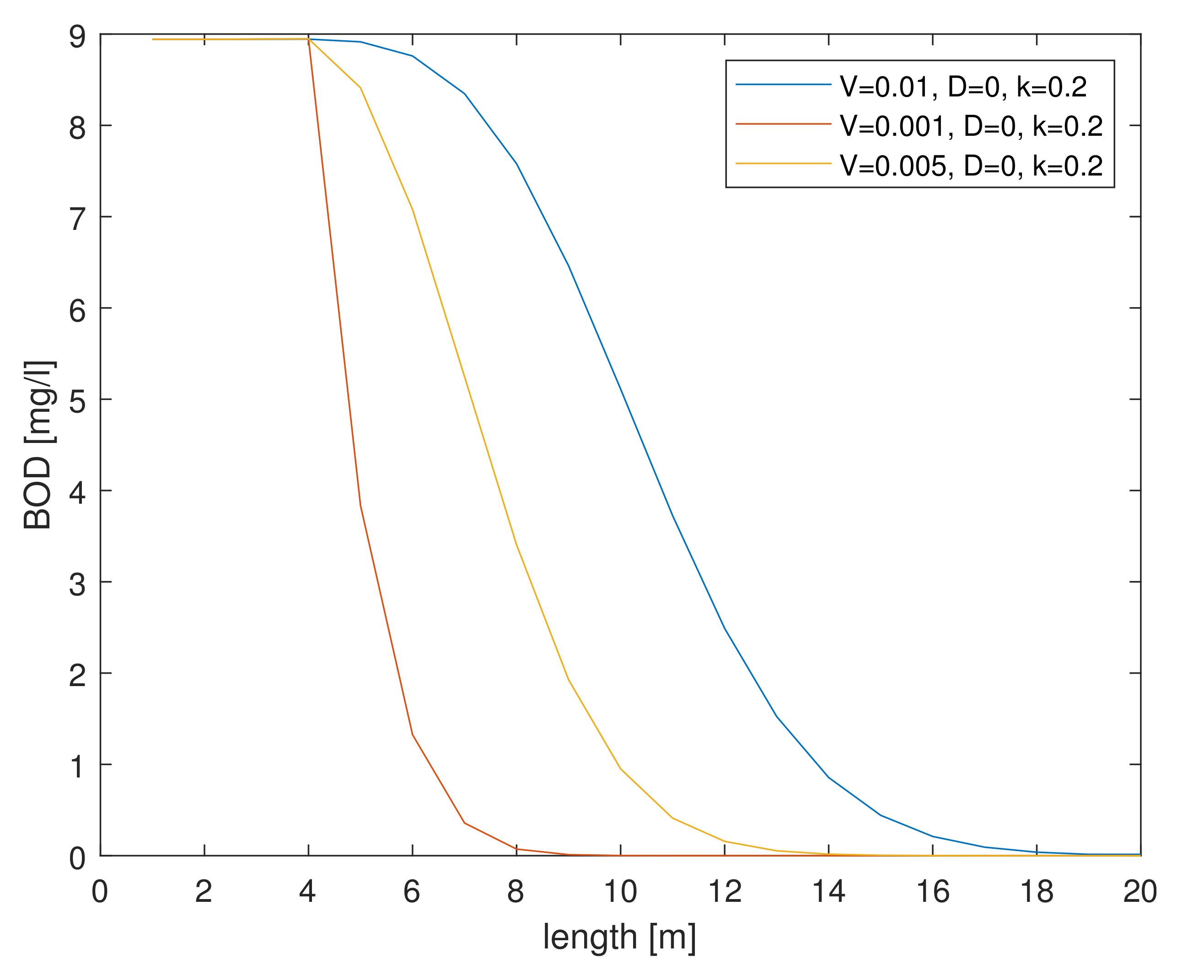
Further considerations included ignoring the phenomenon of diffusion, considering different velocities over the same length, and taking into account the self-cleaning process of the river. The simulation results are shown in Figure 6, and the values used for the simulation are summarised in Table 2. A significant effect of the self-cleaning process can be observed, which influences the faster distribution of pollutants over time and length.

An interesting situation arises at different river velocities. The velocity of the river causes the emerging pollutant to be “entrained” by the river and to decompose along its length (see Figure 7 and

Table 3. The initial values adopted in the simulation studies for the cases shown in Figure 7.

Figure	$\mathit{BOD}\left[\mathbf{mg}/\mathbf{L}\right]$	A	$\mathit{D}\left[{\mathbf{m}}^2/\mathbf{h}\right]$	$\mathit{V}\left[\mathbf{m}/\mathbf{h}\right]$	$\mathit{dz}\left[\mathbf{m}\right]$	$\mathit{dt}\left[\mathbf{h}\right]$
Figure 7a	10	0	0	0.001	0.001	0.0014
Figure 7b	10	0.2	0	0.001	0.001	0.0014

).

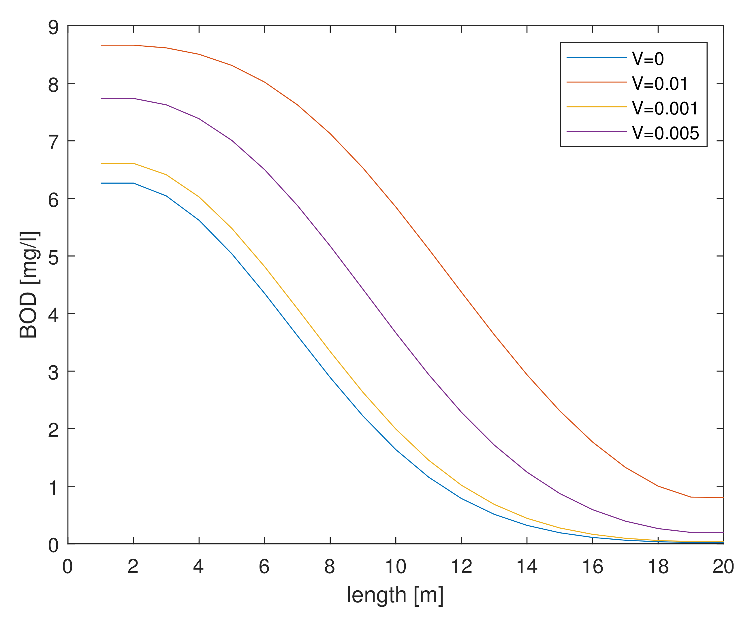
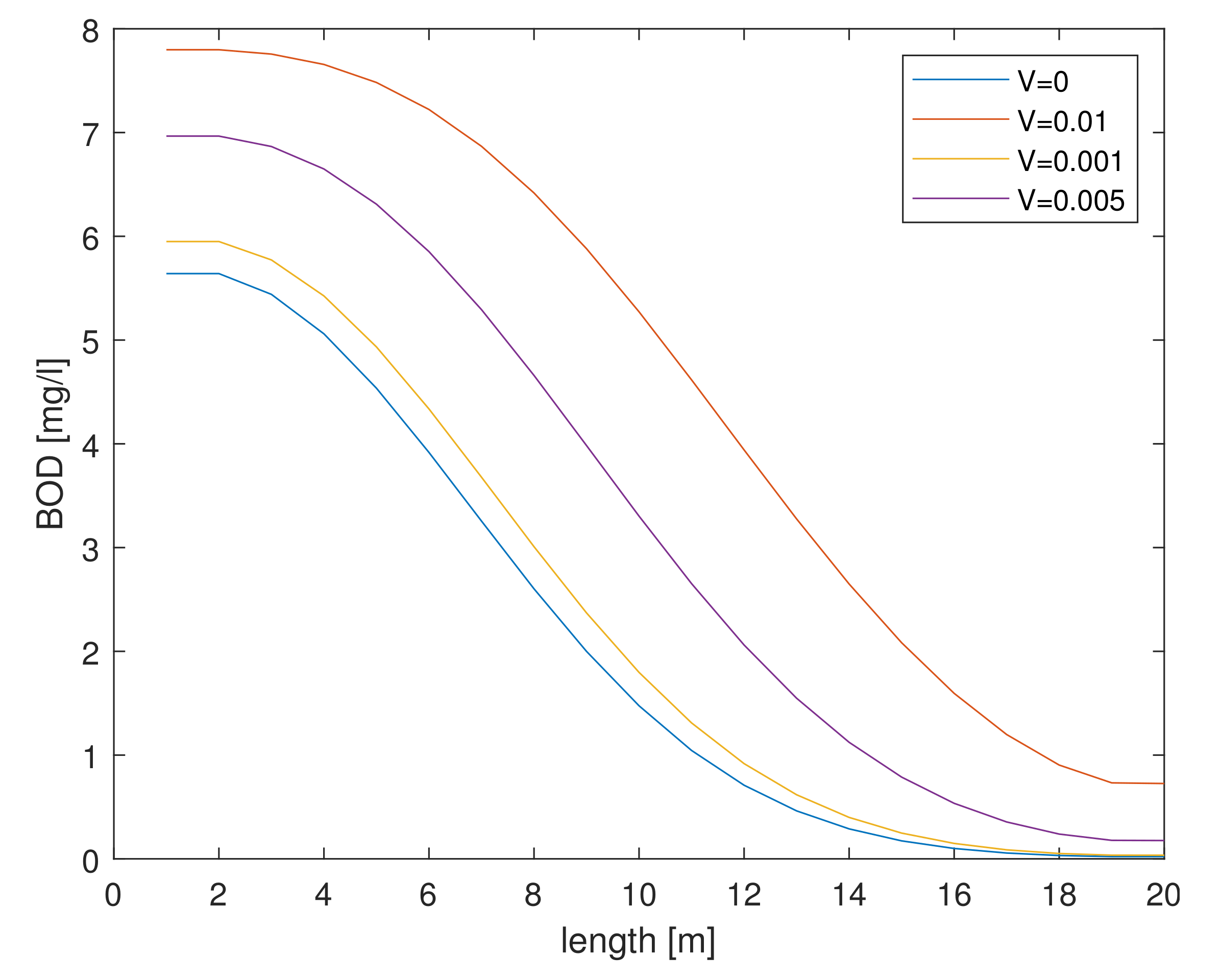
When diffusion is taken into account, the distribution of BOD is strongly influenced by velocity as shown successively in Figure 8, and the values used for the simulations are summarised in

Table 4. The initial values adopted in the simulation studies for the cases shown in Figure 8.

Value	Figure 8a	Figure 8b	Figure 8c
$BOD\left[\mathrm{mg}/\mathrm{L}\right]$	10	10	10
A	0	0	0
$D\left[{\mathrm{m}}^2/\mathrm{h}\right]$	3600 × 5 × 10${}^{-9}$	3600 × 5 × 10${}^{-9}$	3600 × 5 × 10${}^{-9}$
$V\left[\mathrm{m}/\mathrm{h}\right]$	0.001	0.005	0.01
$dz\left[\mathrm{m}\right]$	0.001	0.001	0.001
$dt\left[\mathrm{h}\right]$	0.0014	0.0014	0.0014

. A change in velocity results in a change in BOD concentration values, and a higher velocity results in higher BOD concentrations.

As the velocity increases over the same length of time, the value of the BOD concentration increases. Changes in the BOD concentration at different velocities in the initial time moments are shown in Figure 9.

An interesting phenomenon occurs when diffusion is not considered, as shown in Figure 10 (cf. Figure 8a). Once a pollutant is introduced into the water, the lack of diffusion results in a prolonged period of dangerous conditions in the river, only after the water masses have moved over a certain length and time does the concentration of the pollutant degrade.

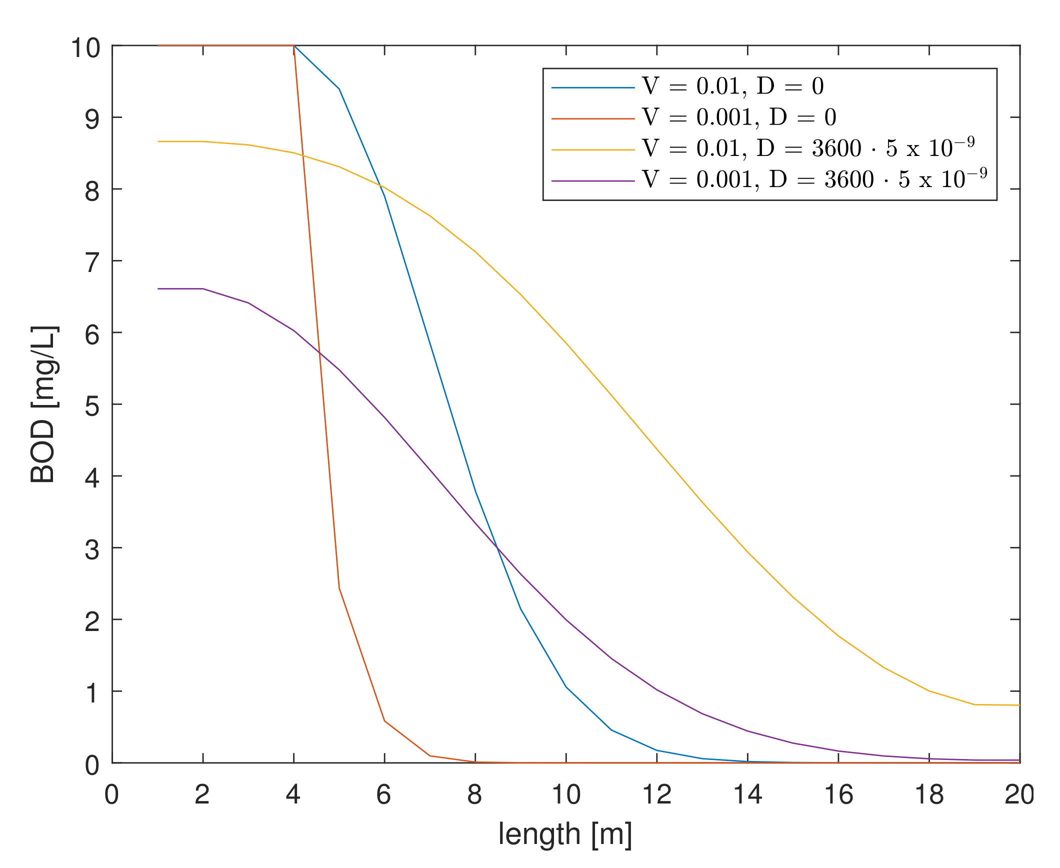
The effect of velocity when diffusion is included and omitted at different velocities is shown in Figure 11. Excluding diffusion after the introduction of a pollutant, the pollutant concentration is higher than when diffusion is allowed for, which results in a faster decomposition of BOD.

Considerations to date have focused on the introduction of pollutants into the river without prolonged perseverance. Another consideration concerns the prolonged stamina of the introduced contaminant for a fixed time, over a given length. This phenomenon can be represented by a grid (Figure 12), which illustrates the persistence of a pollutant at a certain time along a given length, depending on the parameters adopted.

The figure above illustrates the range over which pollution is maintained. The blue dots indicate the tenacity of the pollution over a given length at relevant moments in time, while the white dots are the beginning of the spread of the pollution. The simulation results are shown in Figure 13, and

Table 5. The initial values adopted in the simulation studies for the cases shown in Figure 13 and Figure 15.

Value	Figure 13a	Figure 13b	Figure 15a	Figure 15b
$BOD\left[\mathrm{mg}/\mathrm{L}\right]$	10	10	10	10
A	0	0	0.2	0.2
$D\left[{\mathrm{m}}^2/\mathrm{h}\right]$	3600 × 5 × 10${}^{-9}$	3600 × 5 × 10${}^{-9}$	3600 × 5 × 10${}^{-9}$	3600 × 5 × 10${}^{-9}$
$V\left[\mathrm{m}/\mathrm{h}\right]$	0.001	0.005	0.001	0.01
$dz\left[\mathrm{m}\right]$	0.001	0.001	0.001	0.001
$dt\left[\mathrm{h}\right]$	0.0014	0.0014	0.0014	0.0014

summarises the values used.

It is evident that the initial pollution introduced into the water persists over a long period of time at an appropriate length (cf. Figure 8a,b). In the initial moments of time at a given length, the BOD concentration is high, after which it spreads accordingly over the given area. Depending on the speed of the river, the distribution of pollutants in the river at the same moments of time, along the same length, is different: see Figure 14.

The above considerations concerned the distribution of BOD taking into account the phenomenon of diffusion and disregarding the self-cleaning process of the river. The effect of the self-cleaning process of the river, at different velocities, is shown in Figure 15, and Table 5 summarises the values used for the study. It can be seen that the self-cleaning of the river influences the BOD distribution, resulting in a shorter occurrence of high concentrations of pollutants in a given section of the river.

Figure 16 illustrates the changes in BOD concentration as a function of speed, taking into account the self-cleaning processes. Comparing Figure 14 and Figure 16, the influence of the river’s self-cleaning, on the distribution of pollutants in the section under consideration, can be clearly seen. At the same moments in time, respectively, at the same water mass flow rates, the BOD concentration values are different. The self-cleaning of the river accelerates the breakdown of pollutants, so that the river returns to a clean state more quickly. The value of the concentration at the same moment in time taking into account the self-cleaning process at a rate of $V=0.005$ is $BOD=6.96$ (see Figure 16), without taking into account self-cleaning of the river the value is higher and takes the value of $BOD=7.73$. The detailed BOD values are summarised in

Table 6. BOD values including river self-cleaning process for different water flow rates.

$\mathit{V}\left[\mathbf{m}/\mathbf{h}\right]$	$\mathit{BOD}\left[\mathbf{mg}/\mathbf{L}\right]$
	Figure 14	Figure 16
0	6.26	5.64
0.01	8.66	7.79
0.001	6.60	5.95
0.005	7.73	6.69

.

A different approach to analysis of changes in BOD distribution is shown in Figure 17. The flow rate of the river was taken into account here, but the occurrence of diffusion and the self-cleaning process were neglected. We observe here what was introduced of a tenacious pollutant, introduced over a period of time excluding the diffusion phenomenon leads to prolonged dangerous conditions in the river. Only after a certain time and length does the spread of contamination occur.

In this situation, the key influence on the distribution of pollutants is the velocity of water movement and the diffusion occurring within them. Figure 18 shows the distribution of BOD pollutants at different velocities, excluding and including the diffusion mechanism. The omission of diffusion when maintaining the introduced pollutant for an appropriate time results in a state of prolonged hazardous conditions in the river, while the action of diffusion results in the faster dispersement of the introduced pollutant.

Comparing Figure 11 and Figure 18, we can observe the dynamics of the changes in BOD concentration, which is affected by the persistence of the pollutant for a given moment. During the persistence of the introduced pollutant in the water, the value of BOD concentration at the same velocities is higher. A constant flow of pollutants results in higher concentrations. A summary of the values obtained is shown in

Table 7. BOD values at initial moments of time for different velocities.

$\mathit{BOD}$	$\mathit{V}=0.01$		$\mathit{V}=0.001$
	$\mathit{D}=0$	$\mathit{D}=3600\times$5 × 10${}^{-9}$	$\mathit{D}=0$	$\mathit{D}=3600\times$5 × 10${}^{-9}$
Figure 18	10	8.66	10	6.60
Figure 11	10	7.71	10	5.31

.

Figure 19 shows the effect of velocity on the distribution of pollutants with and without diffusion and self-cleaning, respectively. It can be seen here that at higher velocities of flowing water the distribution of pollutants, including and excluding diffusion effect, takes on similar values. At lower velocities (see Figure 18), it can be seen that the diffusion phenomenon has a strong influence on the distribution of pollutants.

The omission of the diffusion phenomenon regarding the self-cleaning process and different river velocities is shown in Figure 20. Higher water flow velocity causes the introduced pollutants to be “carried away” by the river resulting in a distribution along the entire length of the river.

Conducting simulation experiments without considering diffusion at different velocities with respect to the self-cleaning process, it can be seen that BOD concentration values are high, within the persistence of the pollution, for a long while, and then, they decrease with time and length (Figure 21).

On the basis of the research conducted thus far, on simulation experiments of mathematical models of biochemically polluted water, taking into account the diffusion phenomenon and the influence of individual parameter values on the distribution of pollutants, it can be assumed that at relatively high water flow velocities, the influence of the diffusion phenomenon can be neglected. In objects where the self-purification process is carried out at lower speeds, a large influence of diffusion on the distribution of pollutants was observed, and this phenomenon should be considered in a mathematical model as well as in the algorithmic structure of intelligent module that controls and monitors the quality of water in the river.

4. Conclusions

The paper presents studies on numerical simulations of mathematical models of biochemical water pollutants, for various degrees of model complexity, including the phenomenon of diffusion. The studies analysed phenomena occurring in relation to spatial, time coordinates and variable parameter values in the models. Detailed consideration was given to the biochemical contamination of water, taking into account the phenomenon of diffusion. The experiments conducted concerned the dynamics of the diffusion phenomenon, along the entire length and width of the section of the river under consideration, following a smoothly varying timeline. In fact, the depth of the Wislok is very shallow compared to other dimensions of the river, which resulted in the omission of this parameter. Minimizing the negative effects of serious environmental pollutants is possible, thanks to online monitoring and control systems. As part of the work on the system for monitoring and controlling water quality in rivers, a number of field and laboratory tests were conducted on the Wislok river, which is a river of significant importance for the Podkarpackie voivodeship. The tests were organised at four measuring points: Strzyzow, Zarzecze, Rzeszow and Bialobrzegi. The scope of the field study included the determination of water temperature, measurement of river current velocity, river bed shape and water flow. By contrast, laboratory tests focused on the determination of dissolved oxygen. While designing the presented solution, a mathematical model of a physical object was used, which was a section of a river understood as a certain mathematical abstraction binding together variables characterizing the state of the object, interaction of external signals thereon and its reaction. The pollution load on, the waters of the Wislok, depends on the level of development and industrialization of the catchment area. The pollution level increases after the receipt of municipal and industrial wastewater from various wastewater treatment plants and discharges of municipal and industrial wastewater located along the river. The proposed solution allows real systems to be efficiently designed for river state estimation control. This is important for the control of such objects, particularly, where measurements of certain state vector coordinates require lengthy laboratory service. Currently available technical means and numerical methods allow for the adaptation tasks to be carried out, in a short period of time, with unknown interference characteristics.

References

1. Al Jibouri, A.K.H.; Upreti, S.R.; Wu, J. Optimal control of continuous ozonation of non-biodegradable pollutants. J. Process Control 2018, 66, 1–11. [Google Scholar] [CrossRef]
2. Beveridge, C.; Hossain, F.; Biswas, R.K.; Haque, A.A.; Ahmad, S.K.; Biswas, N.K.; Hossain, M.A.; Bhuyan, M.A. Stakeholder-driven development of a cloud-based, satellite remote sensing tool to monitor suspended sediment concentrations in major Bangladesh rivers. Environ. Model. Softw. 2020, 133, 104843. [Google Scholar] [CrossRef]
3. Li, L.; Wu, J. Spatiotemporal estimation of satellite-borne and ground-level NO2 using full residual deep networks. Remote Sens. Environ. 2021, 254, 112257. [Google Scholar] [CrossRef]
4. Zhang, Y.; Shi, K.; Zhou, Y.; Liu, X.; Qin, B. Monitoring the river plume induced by heavy rainfall events in large, shallow, Lake Taihu using MODIS 250m imagery. Remote Sens. Environ. 2016, 173, 109–121. [Google Scholar] [CrossRef]
5. Gomolka, Z.; Krutys, P.; Twarog, B.; Zeslawska, E. A new approach to spatiotemporal estimation of the river state. J. Process Control 2020, 94, 125–143. [Google Scholar] [CrossRef]
6. Gomolka, Z.; Twarog, B.; Zeslawska, E.; Lewicki, A.; Kwater, T. Using Artificial Neural Networks to Solve the Problem Represented by BOD and DO Indicators. Water 2018, 10, 4. [Google Scholar] [CrossRef] [Green Version]
7. Krutys, P.; Gomolka, Z.; Twarog, B.; Zeslawska, E. Synchronization of the vector state estimation methods with unmeasurable coordinates for intelligent water quality monitoring systems in the river. J. Hydrol. 2019, 572, 352–363. [Google Scholar] [CrossRef]
8. Nearing, G.S.; Moran, M.S.; Scott, R.L.; Ponce-Campos, G. Coupling diffusion and maximum entropy models to estimate thermal inertia. Remote Sens. Environ. 2012, 119, 222–231. [Google Scholar] [CrossRef]
9. Sheng, N.; Tu, Y.-S.; Guo, P.; W, R.-Z.; Fang, H.-P. Diffusing of an Ammonia Molecule in Water in a Very Short Time Period. Phys. Rev. E 2012, 24, 969–970. [Google Scholar] [CrossRef]
10. Sun, Y.; Li, H.; Yang, Q.; Liu, Y.; Fan, J.; Guo, H. Disentangling effects of river inflow and marine diffusion in shaping the planktonic communities in a heavily polluted estuary. Environ. Pollut. 2020, 267, 115414. [Google Scholar] [CrossRef]
11. Harris, H.J.V.T.K.R. Diffusion in Liquids 1st Edition A Theoretical and Experimental Study; Butterworth and Co.: London, UK, 1984. [Google Scholar]
12. Unami, K.; Kawachi, T.; Munir Babar, M.; Itagaki, H. Estimation of diffusion and convection coefficients in an aerated hydraulic jump. Adv. Water Resour. 2000, 23, 475–481. [Google Scholar] [CrossRef]
13. Kumar, A.; Jaiswal, D.K.; Kumar, N. Analytical solutions to one-dimensional advection–diffusion equation with variable coefficients in semi-infinite media. J. Hydrol. 2010, 380, 330–337. [Google Scholar] [CrossRef]
14. Law, A.W.K.; Au, S.K.; Song, J. Stochastic diffusion by progressive waves in turbulence. J. Hydrodyn. Ser. B 2010, 22, 605–610. [Google Scholar] [CrossRef]
15. Huysmans, M.; Dassargues, A. Review of the use of Péclet numbers to determine the relative importance of advection and diffusion in low permeability environments. Hydrogeol. J. 2005, 13, 895–904. [Google Scholar] [CrossRef] [Green Version]
16. Wemaere, I.; Marivoet, J.; Labat, S.; Beaufays, R.; Maes, T. Mol-1 Borehole (April-May 1997): Core Manipulations and Determination of Hydraulic Conductivities in the Laboratory (R-3590); Niras: Brussel, Belgium, 2002. [Google Scholar]
17. Pilotti, M.; Chapra, S.C.; Valerio, G. Steady-state distributed modeling of dissolved oxygen in data-poor, sewage dominated river systems using drainage networks. Environ. Model. Softw. 2019, 111, 153–169. [Google Scholar] [CrossRef]
18. Santín, I.; Pedret, C.; Vilanova, R. Applying variable dissolved oxygen set point in a two level hierarchical control structure to a wastewater treatment process. J. Process Control 2015, 28, 40–55. [Google Scholar] [CrossRef]
19. Wang, Z.; Bai, Y.; He, X.; Tao, B.; Li, T.; Chen, X.; Wang, T.; Gong, F. Estimating particulate organic carbon flux in a highly dynamic estuary using satellite data and numerical modeling. Remote Sens. Environ. 2021, 252, 112116. [Google Scholar] [CrossRef]
20. Canto-Perello, J.; Benitez-Navio, A.; Martin-Utrillas, M.; Martinez-Leon, J.; Curiel-Esparza, J. Water resources sustainability model for wetland conservation based on anonymous expert elicitation. Environ. Model. Softw. 2021, 136, 104952. [Google Scholar] [CrossRef]
21. Moazeni, F.; Khazaei, J.; Mitra, P. An integrated state-estimation framework for interdependent water and energy systems. J. Hydrol. 2020, 590, 125393. [Google Scholar] [CrossRef]
22. Yang, F.; Liang, D. Random-walk simulation of non-conservative pollutant transport in shallow water flows. Environ. Model. Softw. 2020, 134, 104870. [Google Scholar] [CrossRef]
23. Zoboli, O.; Hepp, G.; Krampe, J.; Zessner, M. BaHSYM: Parsimonious Bayesian hierarchical model to predict river sediment yield. Environ. Model. Softw. 2020, 131, 104738. [Google Scholar] [CrossRef]
24. Hawro, P.; Kwater, T.; Pekala, R.; Twarog, B. Soft Sensor with Adaptive Algorithm for Filter Gain Correction in the Online Monitoring System of a Polluted River. Appl. Sci. 2019, 9, 1883. [Google Scholar] [CrossRef] [Green Version]
25. Kwater, T.; Hawro, P.; Bartman, J.; Mazur, D. The algorithm of adaptive determination of amplification of the PD filter estimating object state on the basis of signal measurable on-line. Arch. Control Sci. 2021, 31, 129–143. [Google Scholar] [CrossRef]
26. Park, E. Characterizing channel-floodplain connectivity using satellite altimetry: Mechanism, hydrogeomorphic control, and sediment budget. Remote Sens. Environ. 2020, 243, 111783. [Google Scholar] [CrossRef]
27. Higashino, M.; Stefan, H.G. Oxygen uptake prediction in rivers and streams: A stochastic approach. J. Environ. Manag. 2017, 203, 200–207. [Google Scholar] [CrossRef]
28. Nguyen, T.T.; Keupers, I.; Willems, P. Conceptual river water quality model with flexible model structure. Environ. Model. Softw. 2018, 104, 102–117. [Google Scholar] [CrossRef]
29. Zheng, L.; Chen, C.; Zhang, F.Y. Development of water quality model in the Satilla River Estuary, Georgia. Ecol. Model. 2004, 178, 457–482. [Google Scholar] [CrossRef]
30. Kuang, T.; Du, J.; Zhang, W. Simulation of Water Pollution Diffusion Based on WebGIS. J. Comput. Commun. 2019, 7, 28–38. [Google Scholar] [CrossRef] [Green Version]
Figure 1. Intelligent river water quality control and monitoring system.
Applsci 12 01549 g001
Figure 2. Cross–section of the riverbed and current velocities—Lutoryz (a) and Smolarzyny (b).
Applsci 12 01549 g002
Figure 3. Distribution of BOD including diffusion.
Applsci 12 01549 g003
Figure 4. Distribution of BOD including diffusion at different times t.
Applsci 12 01549 g004
Figure 5. BOD distribution for V = 0.005 (a) V = 0.01 (b) including the self-cleaning process.
Applsci 12 01549 g005
Figure 6. BOD distribution for V = 0.005 (a) excluding the self-cleaning process and (b) including the self-cleaning process.
Applsci 12 01549 g006
Figure 7. BOD distribution excluding the self-cleaning process (a) and including the self-cleaning process (b).
Applsci 12 01549 g007
Figure 8. BOD distribution including diffusion for V = 0.001 (a) V = 0.005 (b) V = 0.01 (c).
Applsci 12 01549 g008
Figure 9. BOD distribution including diffusion at different velocities in the same time moments.
Applsci 12 01549 g009
Figure 10. BOD distribution excluding diffusion, no self-cleaning process for V = 0.001 .
Applsci 12 01549 g010
Figure 11. BOD distribution at different velocities in the same moments of time including diffusion D > 0 and excluding diffusion D = 0 .
Applsci 12 01549 g011
Figure 12. Grid representing the distribution of pollution excitations over length and time.
Applsci 12 01549 g012
Figure 13. BOD distribution including diffusion for V = 0.001 (a) V = 0.005 (b).
Applsci 12 01549 g013
Figure 14. BOD distribution, including diffusion D > 0 , at different velocities in the same time moments.
Applsci 12 01549 g014
Figure 15. BOD distribution including diffusion for V = 0.001 (a) V = 0.01 (b) including the self-cleaning process.
Applsci 12 01549 g015
Figure 16. BOD distribution at different velocities in the same time steps.
Applsci 12 01549 g016
Figure 17. BOD distribution excluding diffusion and no self-cleaning process for V = 0.001 .
Applsci 12 01549 g017
Figure 18. BOD distribution for different velocities including and excluding diffusion.
Applsci 12 01549 g018
Figure 19. BOD distribution for different velocities, excluding diffusion D = 0 and including diffusion D > 0 .
Applsci 12 01549 g019
Figure 20. BOD distribution including the self-cleaning process without diffusion for V = 0.001 (a) V = 0.01 (b).
Applsci 12 01549 g020
Figure 21. BOD distribution excluding diffusion, at different velocities in the same moments of time, considering the self-cleaning process.
Applsci 12 01549 g021