
Techniques, Tricks, and Stratagems of Oral Cavity Computed Tomography and Magnetic Resonance Imaging

 , , ,
, , ,  ,
, 
Abstract
:1. Introduction
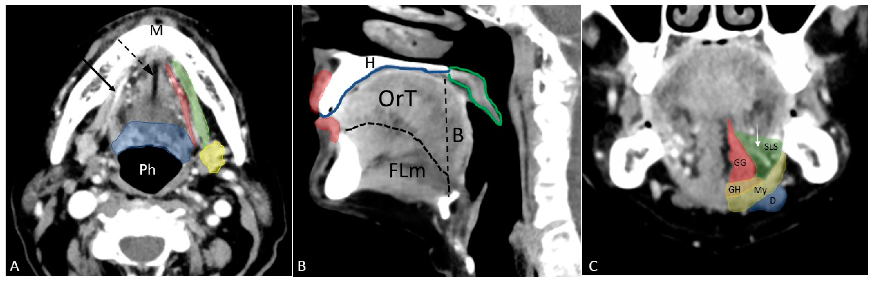
2. Anatomy
- Anteriorly: lips;
- Posteriorly: circumvallate papillae, tonsillar pillars, and soft palate;
- Superiorly: hard palate;
- Inferiorly: floor of the mouth and mandibular alveolar mucosal surface;
- Laterally: gingival–buccal margins on both sides;
- Body of the tongue, the anterior two-thirds since the posterior third is a part of oropharynx;
- Floor of the mouth, located below the lingual surface and bounded inferiorly by the mylohyoid muscle;
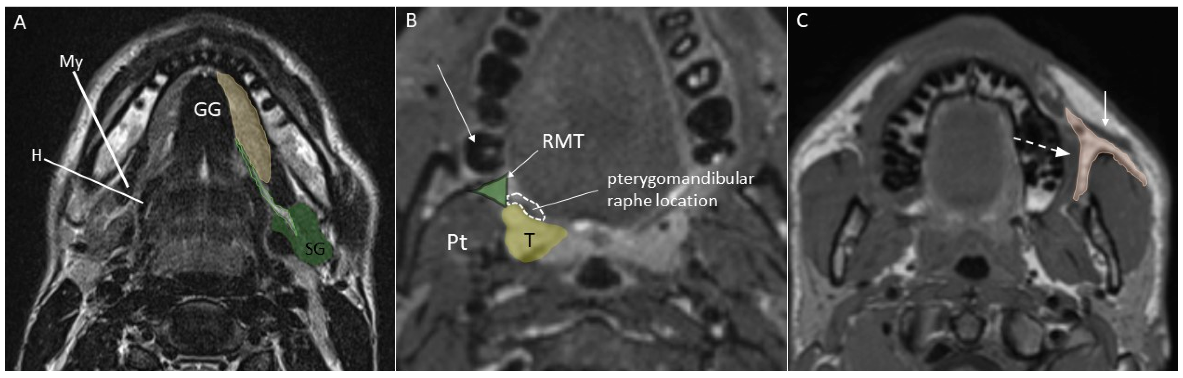
- Lip, mainly formed by the orbicularis oris muscle;
- Buccal space, a fat-containing site between the buccinator and platysma muscles;
- Gingiva, the mucosa overlying the alveolar processes of the jaws;
- Retromolar trigone, a triangular-shaped site formed by the mucosa posterior to the lower jaw third molar;
- Hard palate, the bony structure that forms the palate anteriorly;
3. Imaging Techniques
4. MSCT and MRI Acquisition Protocols
4.1. MSCT
4.2. MRI
- Contrast-enhanced-T1 sequences are excellent both for the detection of enhanced masses—that sometimes are visible only after contrast administration as areas of enhancement—and perineural spread by the direct visualisation of thickened and enhanced nerves;
- Axial T2 combined with multiplanar contrast-enhanced-T1 sequences for the visualisation of tongue extrinsic muscle involvement;
- Unenhanced T1 and T2 sequences for cortical bone erosions;
- Unenhanced T1, T2 SPACE, and contrast-enhanced-T1 sequences for bone marrow involvements;
- T2, contrast-enhanced-T1, and DWI for the assessment of lymph nodes.
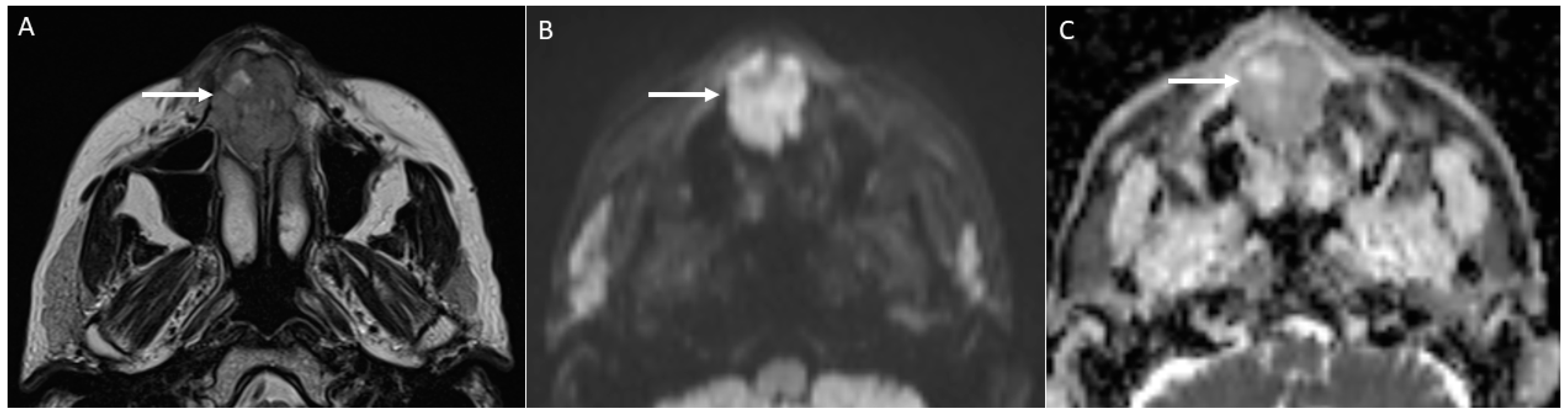
4.2.1. DWI
- Characterise oral lymphoma since it shows the lowest ADC values (<0.7 × 10⁻³ mm2/s) because of its high cellularity (strongly crammed lymphocytes) [30]. Abscesses and lymphomas can show an overlap of ADC values around 0.7 × 10⁻³ mm2/s. However, the differential diagnosis between them is normally carried out considering both the clinical assessment and unenhanced and enhanced morphologic MRI sequences. On the contrary, poorly differentiated carcinomas can assume ADC values similar to lymphomas supported by the increase in cellularity as the grade of the tumour increases, thus making the differential diagnosis more complex [34].
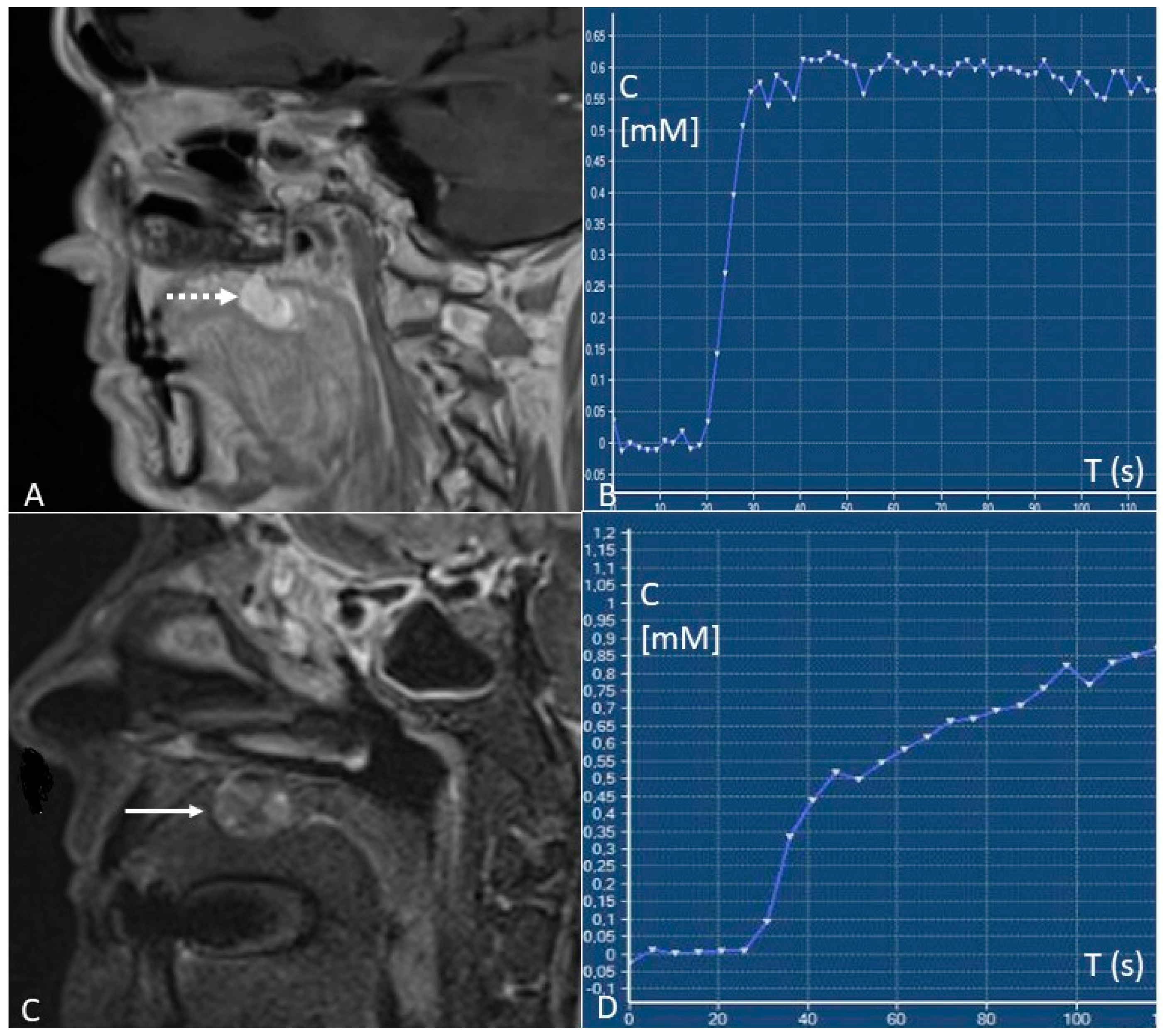
4.2.2. DCE–PWI
- Early identification of locoregional recurrences by the differentiation between local recurrences and post-treatment changes. Relapses show type B or C time/intensity curves (wash-in with wash-out or plateau), whereas post-treatment changes predominantly show type A curves (progressive enhancement). “Time factor” is crucial since a too-short interval of time from surgery or radiotherapy (<3–4 months) can determine false positives due to the presence of inflammatory areas and oedema with vivid enhancement [41];
- Predict pathological stages of oral cancer. For oral tongue squamous cell carcinomas, that are the most frequent malignancies of the oral cavity, staging before treatment is essential since a stage I-II TNM can be treated with a single modality therapy (preferably surgery), whereas stage III-IV TNM have to be treated with multi-modality therapy. Depending on the TNM stage, oral cavity cancers have a different microvasculature function reflected in different pharmacokinetic parameters at the quantitative DCE-MRI analysis. Stage I–II tumours show higher Ktrans values than stage III-IV tumours (0.149 ± 0.080 vs. 0.106 ± 0.057 min−1) [42];
- Differentiate metastatic from normal lymph nodes. Yan et al. [45] found that the value of Ktrans in nodal metastases from squamous cell carcinoma is higher than benign nodes (0.328 ± 0.111 vs. 0.141 ± 0.065 min−1);
- Predict tumour response to treatment. Although with a high metastatic potential, highly perfused tumours are considered to have a better therapeutic response because they receive a great amount of chemotherapy and are more sensitive to radiotherapy. The most accurate pre-therapy DCE-MRI parameter for predicting tumour treatment response is Ktrans. Higher pre-therapy Ktrans values are associated with a better response to therapy, with threshold values > 0.41 to 0.84 min−1 [46].
5. Dynamic Manoeuvres and Stratagems for the Study of the Oral Cavity via MSCT and MRI
- 1.
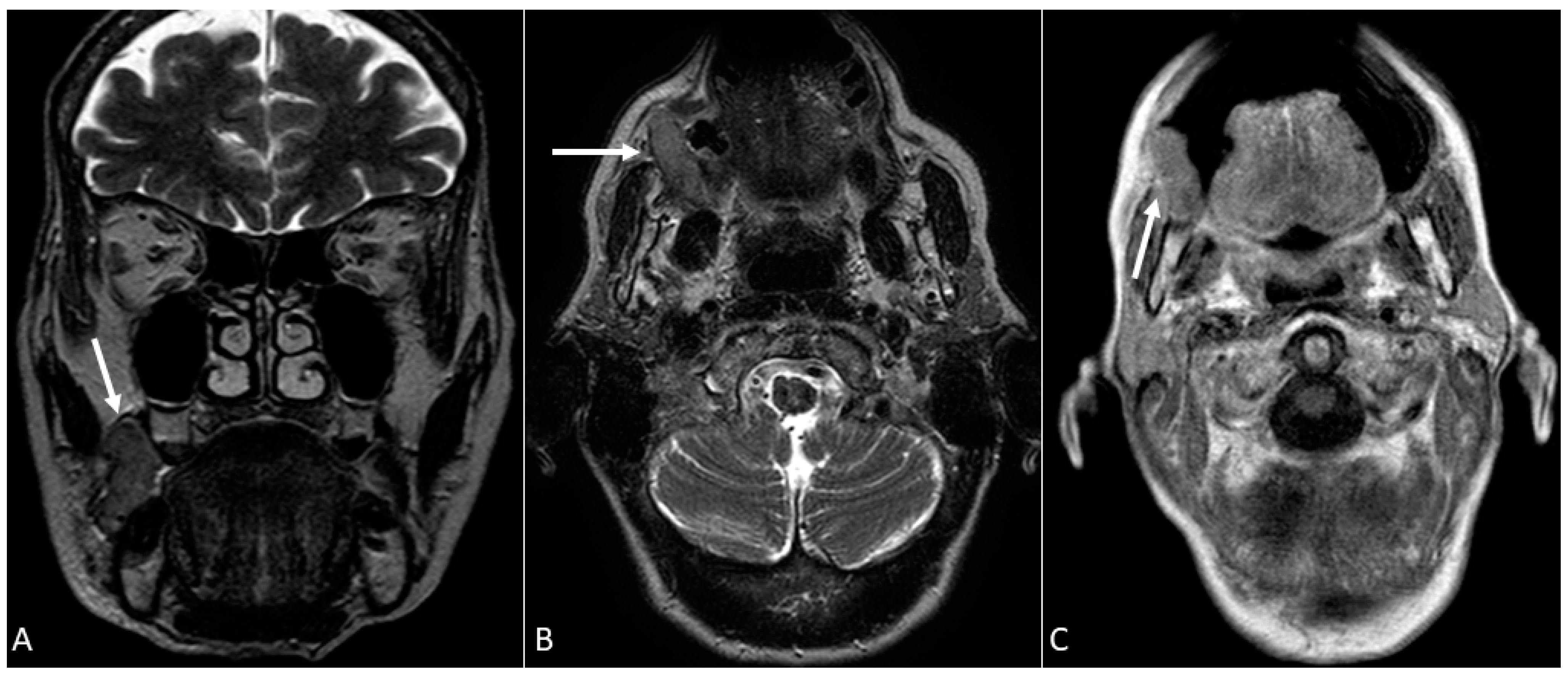
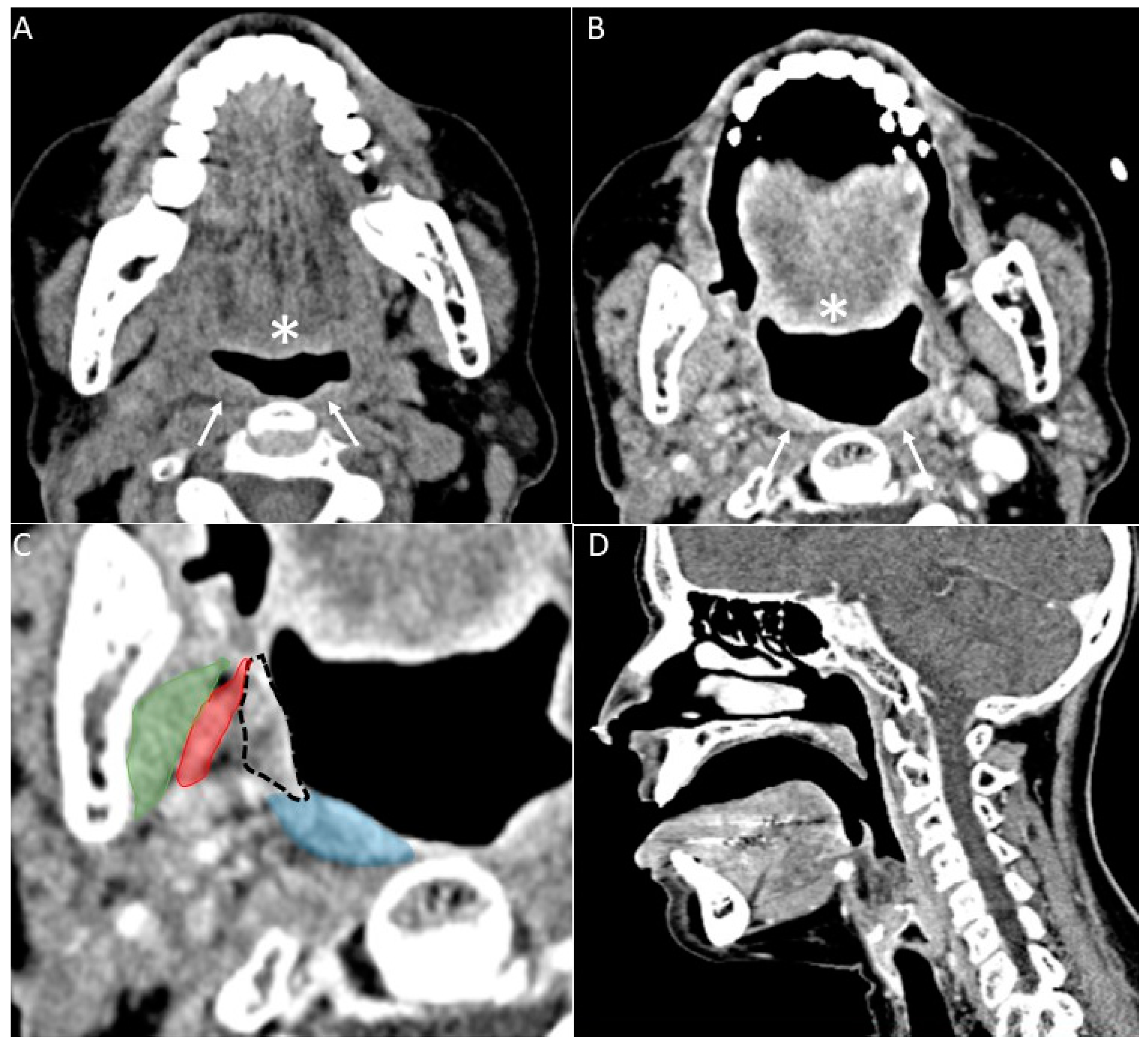
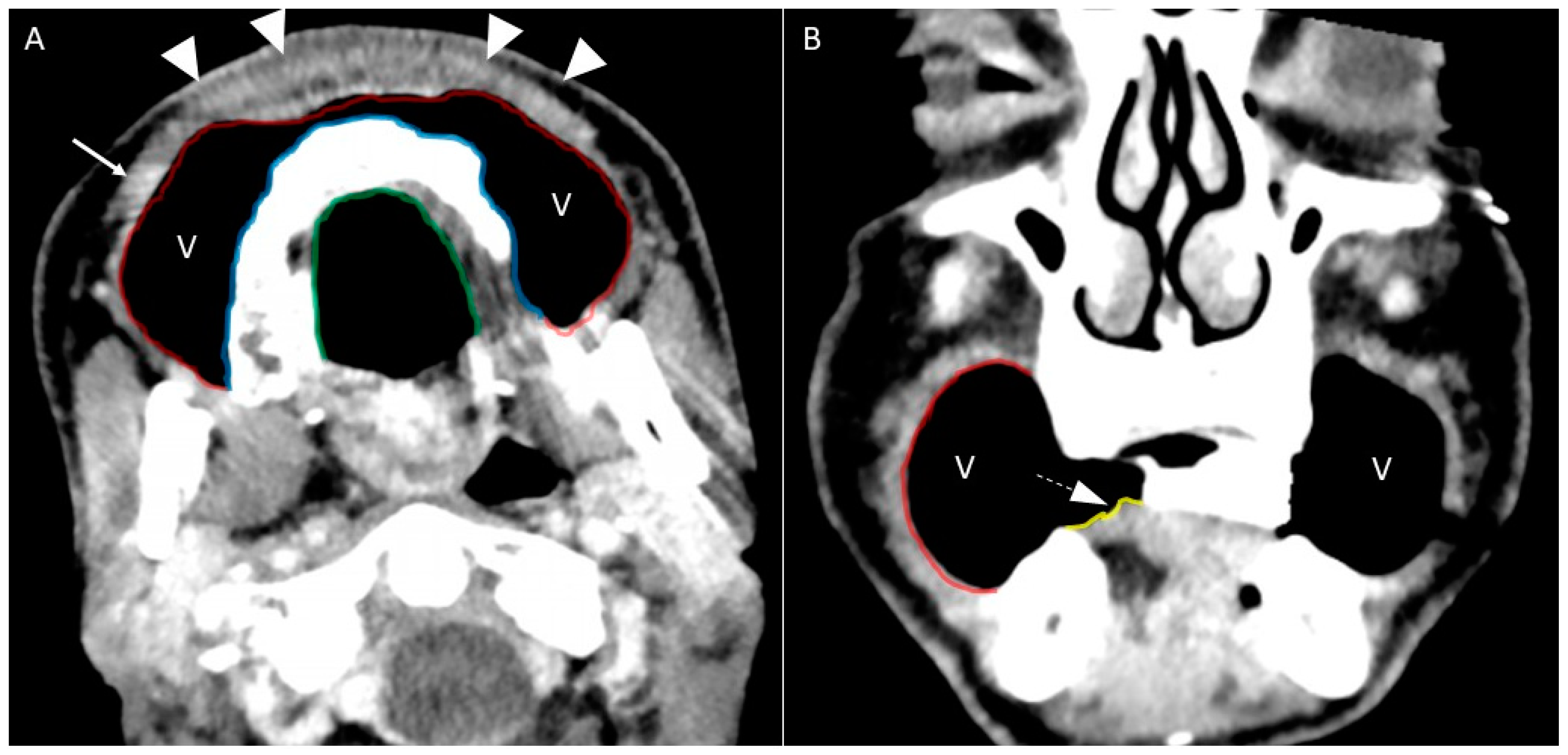
- Puffed cheek technique. The vestibule of the mouth is a virtual cavity due to the contact between the mucosa of the lip, cheek, and gingiva. Puffed cheek technique helps to determine if the lesion is arising from the buccal, gingival, or lingual mucosal surface since patients blow uniformly through pursed lips and the mucosal surfaces appear separated from each other. Therefore, the vestibular cavity can be appreciated as an air-filled horse-shoe-shaped space both on MSCT and MRI (Figure 10 and Figure 11).
- 2.
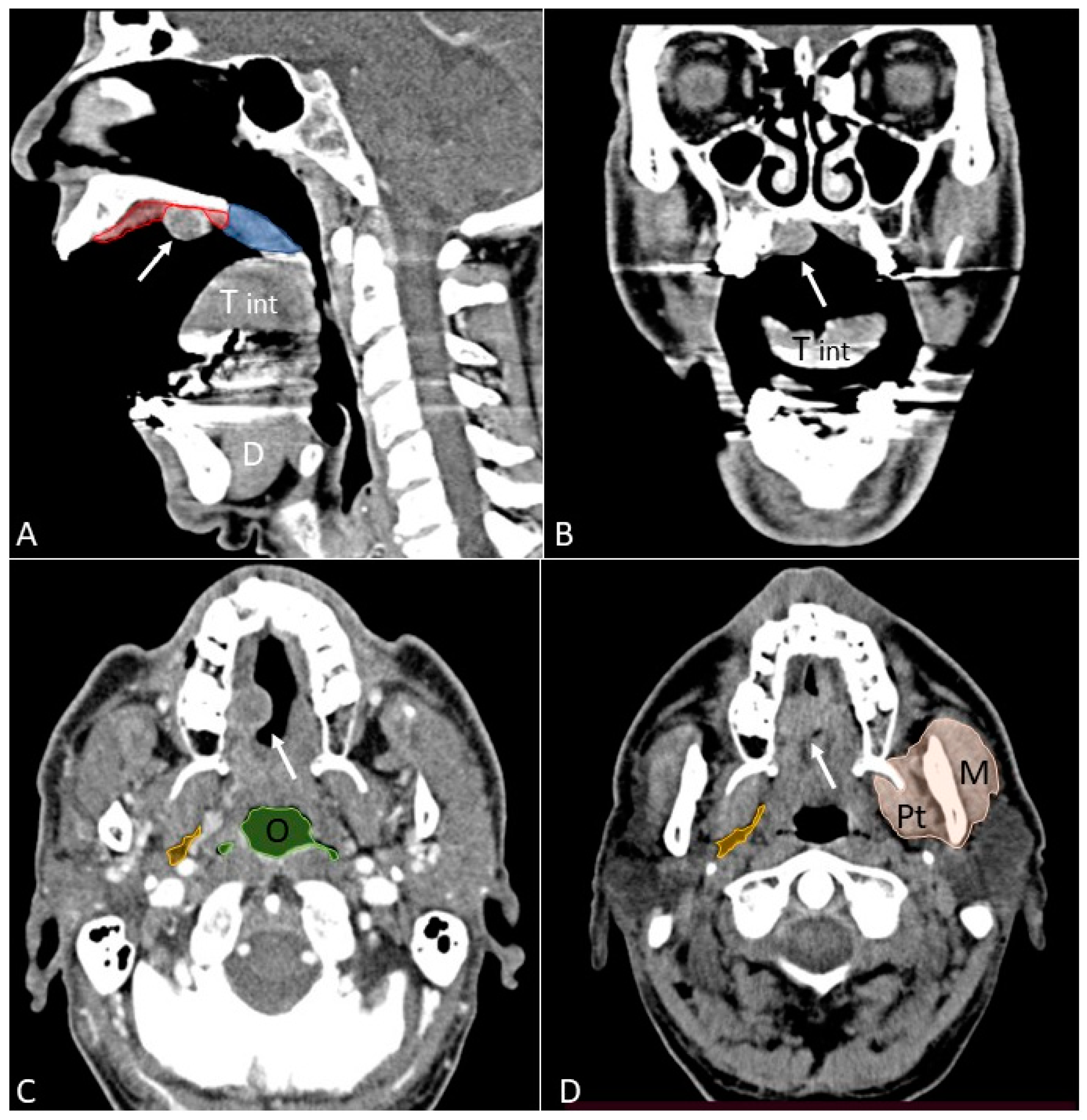
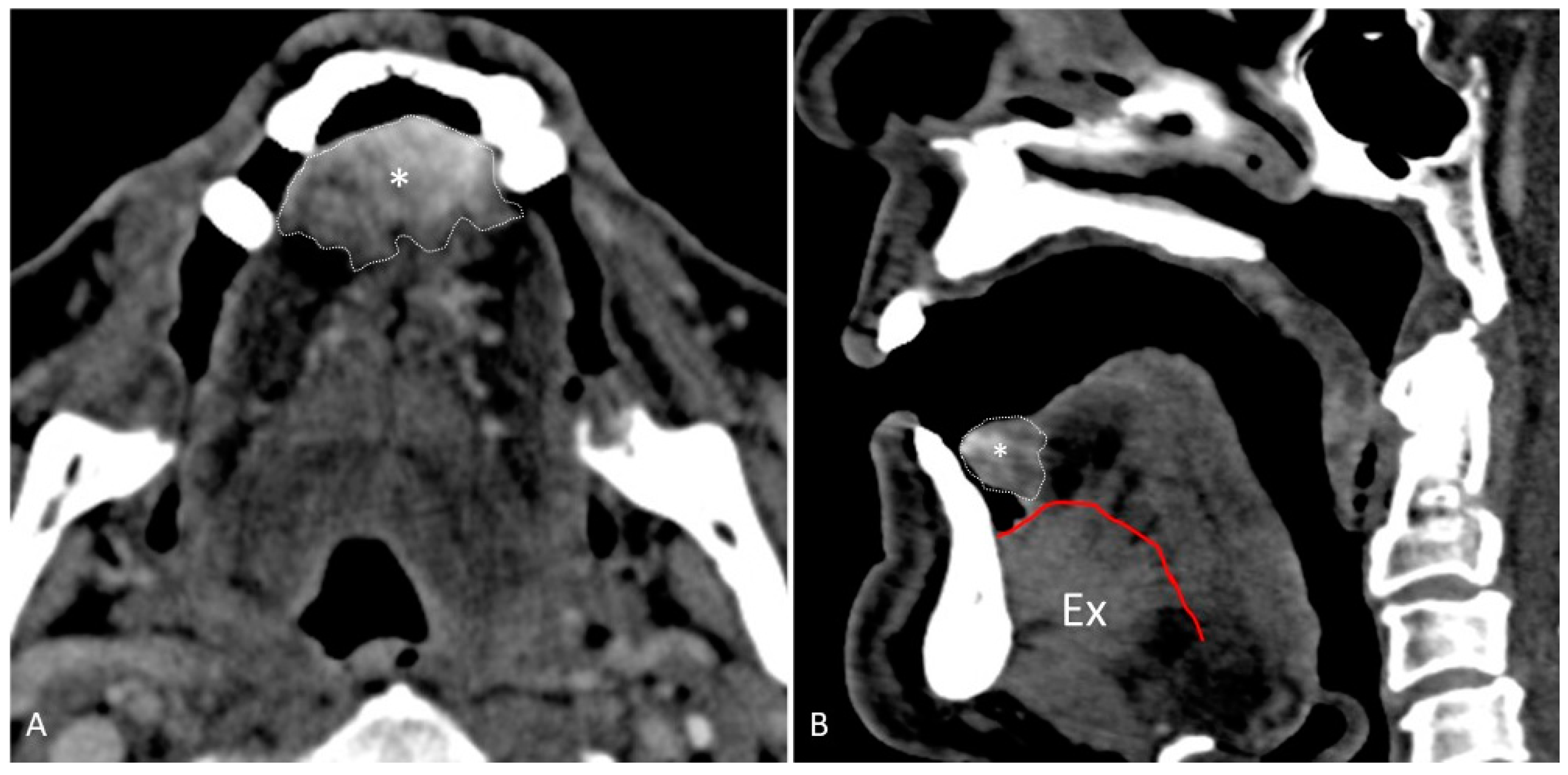
- Open mouth technique. Patients open their mouth and the acquisition is obtained with quiet respiration. A device (i.e., a 50 mL syringe) can be used between teeth to ensure the maintenance of the right position [28]. It allows the separation of the palatal mucosa from the muscular component of the tongue clarifying the exact origin, infiltration, and thickness of tumoural masses (Figure 12 and Figure 13).
- 3.
- 4.
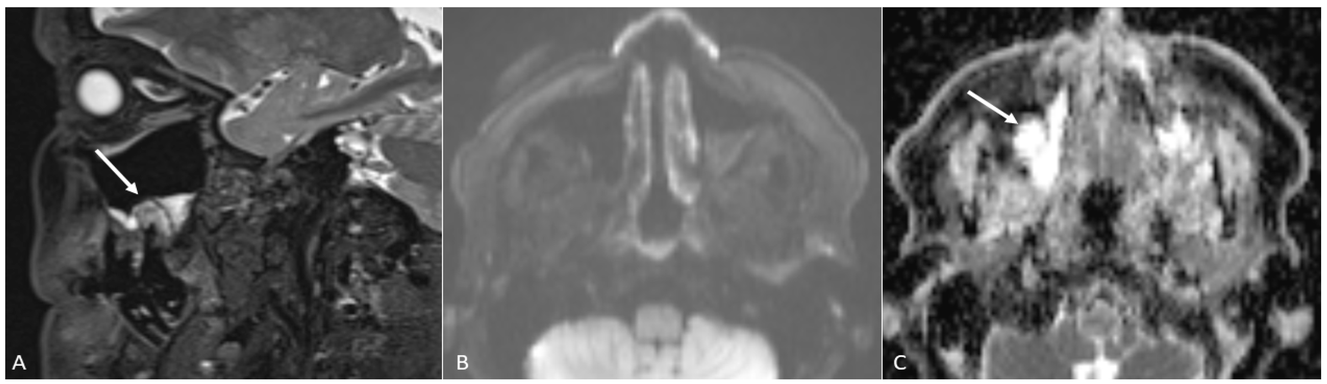
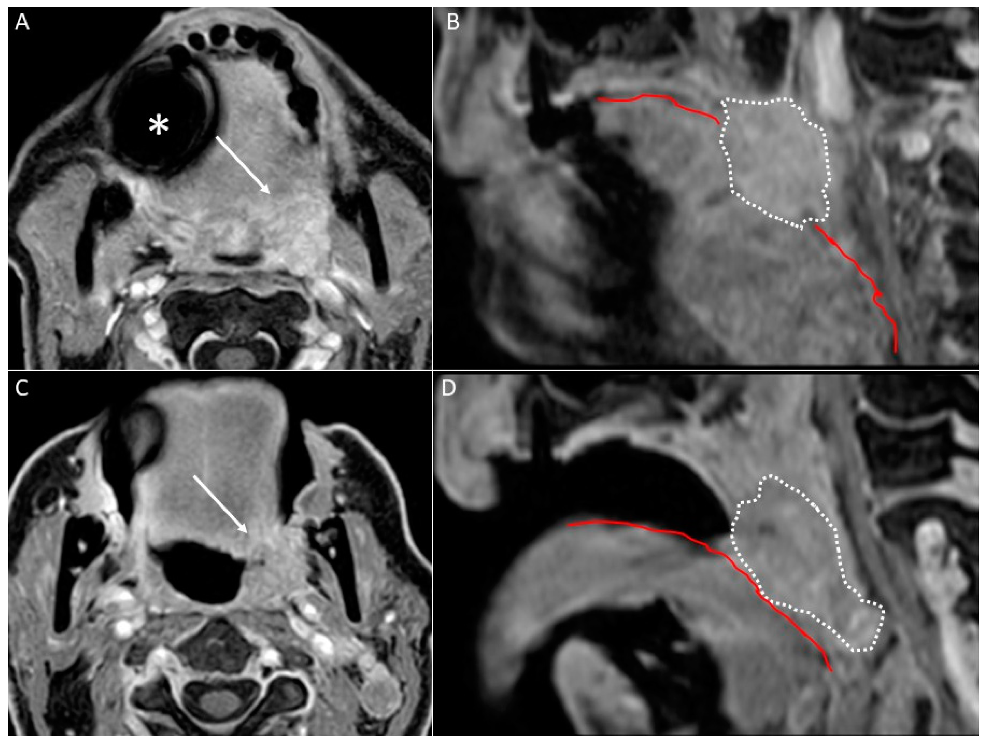
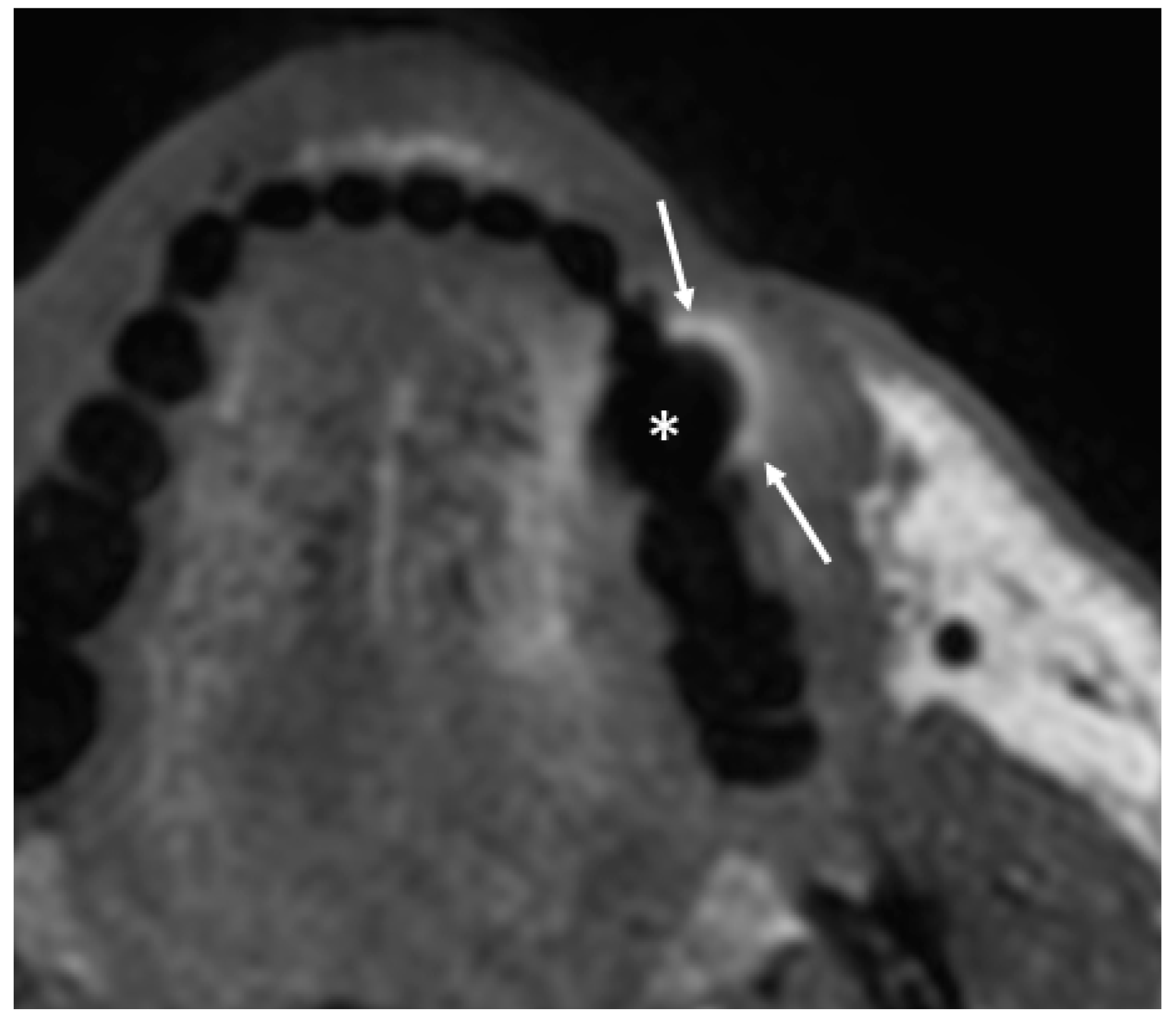
- Water distension of the oral vestibule. This technique is exclusively used on MRI examinations since MRI has a high contrast for liquids by using specific sequences, especially T2 sequences. Water distension of the oral vestibule is performed by asking patients to drink 20–40 mL of still water and keep it in the mouth for the time necessary to acquire the images (T2 and pre- and post-contrast T1 sequences) [47]. This manoeuvre distends the oral vestibule and the presence of water provides excellent natural contrast between the lesion and the adjacent mucosal surfaces (Figure 17).
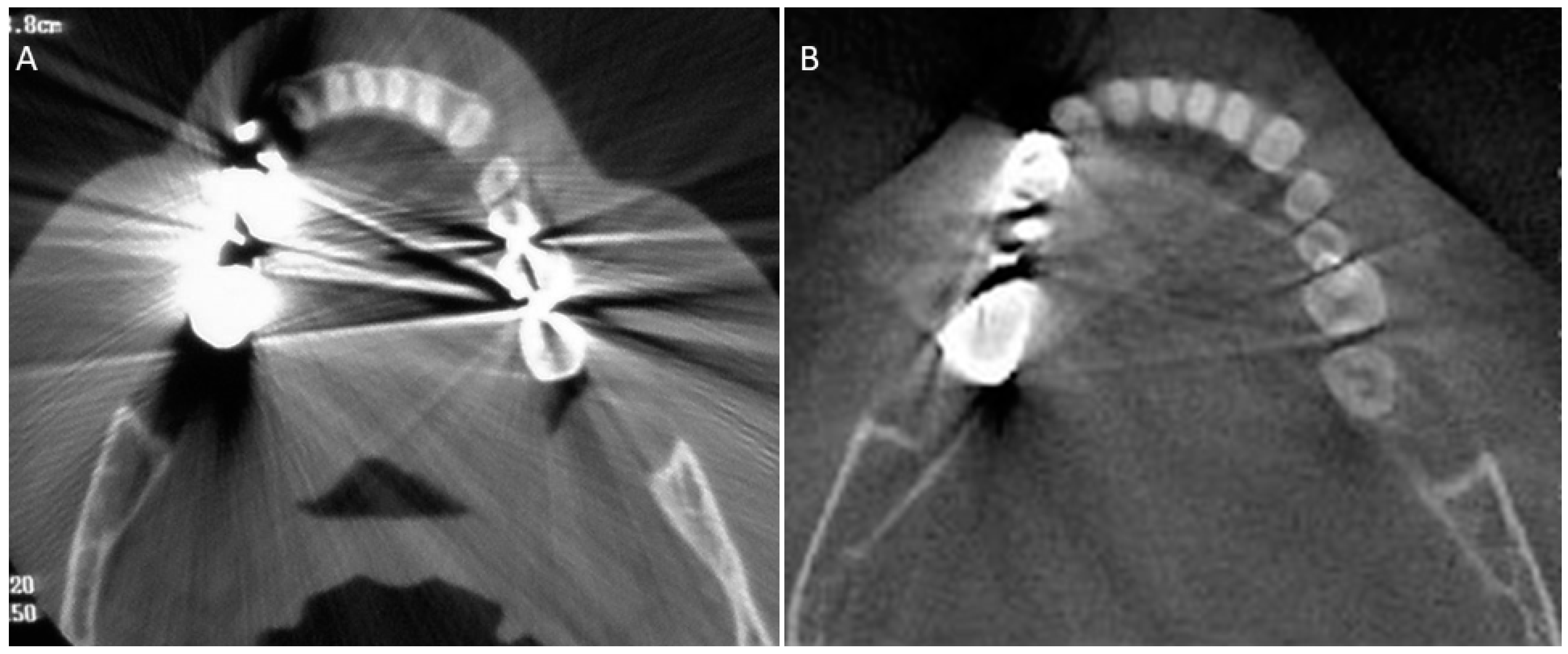
6. Metal Artifacts and Stratagems for Their Reduction
6.1. MSCT
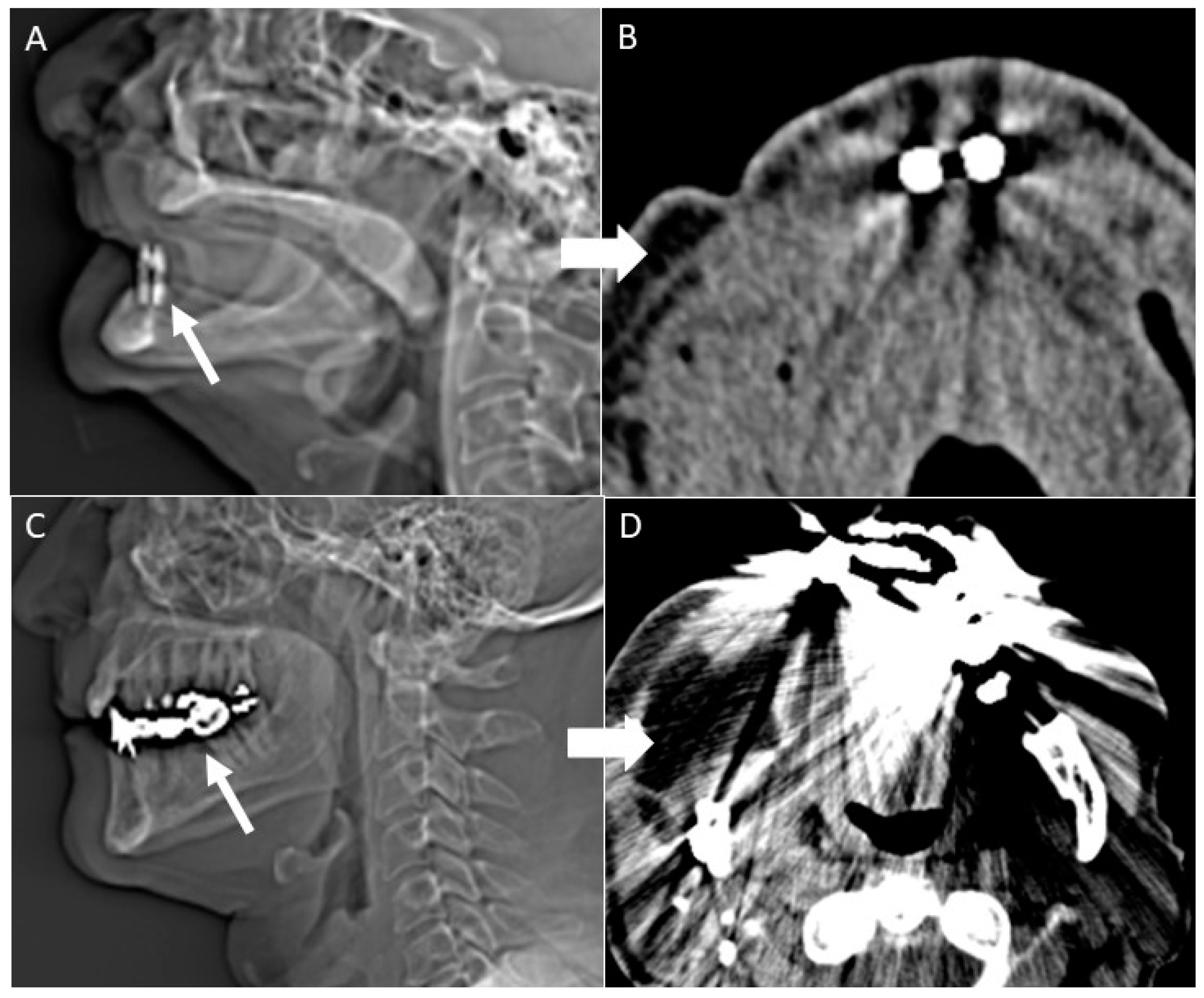
- Gantry tilt scanning. Patients have to be positioned with tooth occlusal surfaces perpendicular to the table; the gantry tilt angle used is ≥20 degrees. In the post-processing phase the oblique images obtained are reconstructed to transverse images with information on the table position [53];
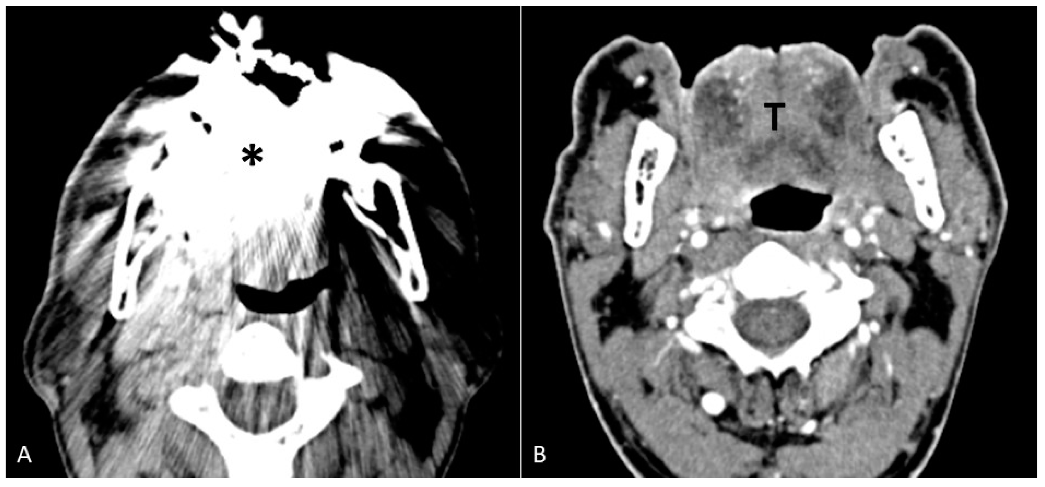
- Open mouth dynamic manoeuvre. See the above-mentioned paragraph and Figure 14);
6.2. MRI
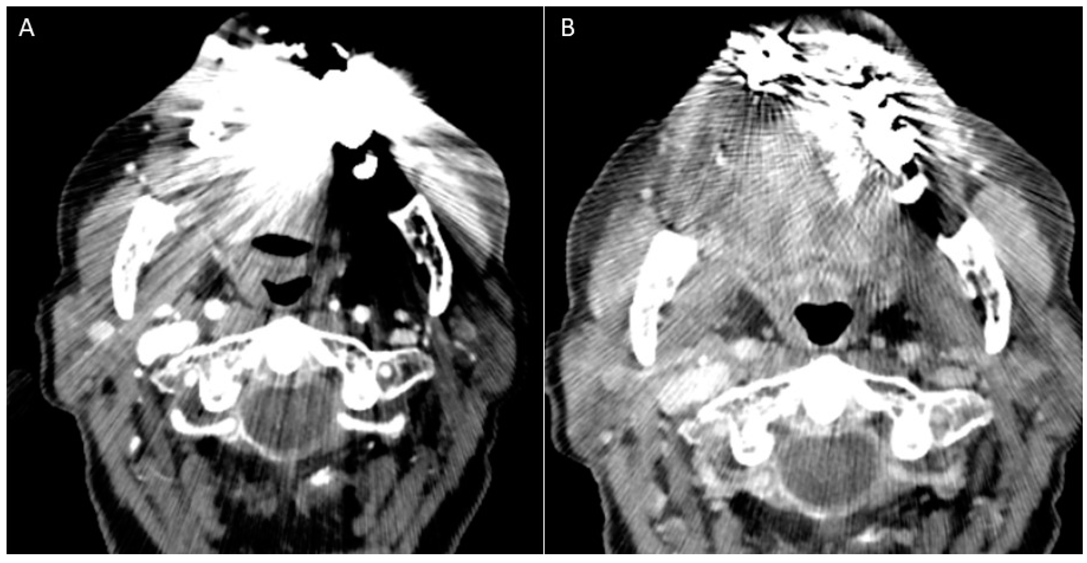
- Spin-echo sequences with modified parameters (i.e., echo time, matrix, bandwidth, slice thickness, and echo train); high bandwidth per voxel, 3D spatial encoding, high-resolution matrix, and multi-echo spin-echo sequences or turbo/fast spin-echo sequences. Spin-echo sequences are less sensitive to susceptibility effects thanks to a 180° radiofrequency pulse that refocuses the spins diminishing the phase shifts in the voxel and therefore the field inhomogeneity [58];
- Gradient echo sequence with a very short echo time. These sequences are metal-sensitive and the signal loss is due to the intravoxel dephasing. Shortening the echo time and decreasing the voxel size can diminish the intravoxel dephasing and therefore the artifacts [58];
- Optimised metal artifact-free sequences with a specific intensity and size of susceptibility artifacts, including the multi-acquisition variable-resonance image combination (MAVRIC) and slice encoding for metal artifact correction (SEMAC) techniques. SEMAC uses a slice selection gradient for excitation and a view-angle tilting compensation gradient for readout. MAVRIC and SEMAC show significantly smaller artifact extent than fast spin-echo imaging [59].
7. Conclusions
Funding
Institutional Review Board Statement
Informed Consent Statement
Data Availability Statement
Conflicts of Interest
References
- Peres, M.A.; Macpherson, L.M.; Weyant, R.J.; Daly, B.; Venturelli, R.; Mathur, M.R.; Listl, S.; Celeste, R.K.; Guarnizo-Herreño, C.C.; Kearns, C.; et al. Oral diseases: A global public health challenge. Lancet 2019, 394, 249–260, Erratum in Lancet 2019, 394, 1010. [Google Scholar] [CrossRef]
- Gondak, R.; Da Silva-Jorge, R.; Jorge, J.; Lopes, M.; Vargas, P.A. Oral pigmented lesions: Clinicopathologic features and review of the literature. Med. Oral Patol. Oral Cir. Bucal. 2012, 17, e919–e924. [Google Scholar] [CrossRef] [PubMed]
- Montero, P.H.; Patel, S.G. Cancer of the Oral Cavity. Surg. Oncol. Clin. N. Am. 2015, 24, 491–508. [Google Scholar] [CrossRef] [PubMed] [Green Version]
- Farah, C. Narrow Band Imaging-guided resection of oral cavity cancer decreases local recurrence and increases survival. Oral Dis. 2018, 24, 89–97. [Google Scholar] [CrossRef]
- Ridgway, J.M.; Armstrong, W.B.; Guo, S.; Mahmood, U.; Su, J.; Jackson, R.P.; Shibuya, T.; Crumley, R.L.; Gu, M.; Chen, Z.; et al. In Vivo Optical Coherence Tomography of the Human Oral Cavity and Oropharynx. Arch. Otolaryngol.—Head Neck Surg. 2006, 132, 1074–1081. [Google Scholar] [CrossRef] [Green Version]
- Mazziotti, S.; Ascenti, G.; Scribano, E.; Mileto, A.; Racchiusa, S.; Visalli, C.; Salamone, I.; Vinci, S.; Blandino, A. CT-MR integrated diagnostic imaging of the oral cavity: Neoplastic disease. La Radiol. Med. 2012, 118, 123–139. [Google Scholar] [CrossRef] [PubMed]
- Law, C.P.; Chandra, R.; Hoang, J.K.; Phal, P.M. Imaging the oral cavity: Key concepts for the radiologist. Br. J. Radiol. 2011, 84, 944–957. [Google Scholar] [CrossRef] [PubMed] [Green Version]
- Nardi, C.; Talamonti, C.; Pallotta, S.; Saletti, P.; Calistri, L.; Cordopatri, C.; Colagrande, S. Head and neck effective dose and quantitative assessment of image quality: A study to compare cone beam CT and multislice spiral CT. Dentomaxillofac. Radiol. 2017, 46, 20170030. [Google Scholar] [CrossRef] [PubMed]
- Ng, S.-H.; Yen, T.-C.; Liao, C.-T.; Chang, J.T.-C.; Chan, S.-C.; Ko, S.-F.; Wang, H.-M.; Wong, H.-F. 18F-FDG PET and CT/MRI in oral cavity squamous cell carcinoma: A prospective study of 124 patients with histologic correlation. J. Nucl. Med. 2005, 46, 1136–1143. [Google Scholar]
- King, K.G.; Kositwattanarerk, A.; Genden, E.; Kao, J.; Som, P.M.; Kostakoglu, L. Cancers of the Oral Cavity and Oropharynx: FDG PET with Contrast-enhanced CT in the Posttreatment Setting. RadioGraphics 2011, 31, 355–373. [Google Scholar] [CrossRef] [Green Version]
- Linz, C.; Brands, R.C.; Herterich, T.; Hartmann, S.; Müller-Richter, U.; Kübler, A.C.; Haug, L.; Kertels, O.; Bley, T.A.; Dierks, A.; et al. Accuracy of 18-F Fluorodeoxyglucose Positron Emission Tomographic/Computed Tomographic Imaging in Primary Staging of Squamous Cell Carcinoma of the Oral Cavity. JAMA Netw. Open 2021, 4, e217083. [Google Scholar] [CrossRef] [PubMed]
- Roele, E.D.; Timmer, V.C.M.L.; Vaassen, L.A.A.; van Kroonenburgh, A.M.J.L.; Postma, A.A. Dual-Energy CT in Head and Neck Imaging. Curr. Radiol. Rep. 2017, 5, 19. [Google Scholar] [CrossRef] [PubMed] [Green Version]
- Subramaniam, N.; Poptani, H.; Schache, A.; Bhat, V.; Iyer, S.; Sunil, H.; Chandrasekhar, N.H.; Pillai, V.; Chaturvedi, P.; Krishna, S.H.; et al. Imaging advances in oral cavity cancer and perspectives from a population in need: Consensus from the UK-India oral cancer imaging group. J. Head Neck Physicians Surg. 2021, 9, 4. [Google Scholar] [CrossRef]
- Drage, N.; Qureshi, S.; Lingam, R. Imaging patients with cancer of the oral cavity. Br. Dent. J. 2018, 225, 827–832. [Google Scholar] [CrossRef]
- Varma, R.; Tibrewala, S.; Roplekar, S. Computed Tomography Evaluation of Oral Cavity and Oropharyngeal Cancers. Int. J. Otorhinolaryngol. Clin. 2013, 5, 51–62. [Google Scholar] [CrossRef] [Green Version]
- Filauro, M.; Missale, F.; Marchi, F.; Iandelli, A.; Carobbio, A.L.C.; Mazzola, F.; Parrinello, G.; Barabino, E.; Cittadini, G.; Farina, D.; et al. Intraoral ultrasonography in the assessment of DOI in oral cavity squamous cell carcinoma: A comparison with magnetic resonance and histopathology. Eur. Arch. Oto-Rhino-Laryngol. 2020, 278, 2943–2952. [Google Scholar] [CrossRef]
- Lechuga, L.; Weidlich, G.A. Cone Beam CT vs. Fan Beam CT: A Comparison of Image Quality and Dose Delivered Between Two Differing CT Imaging Modalities. Cureus 2016, 8, e778. [Google Scholar] [CrossRef] [Green Version]
- Nardi, C.; Salerno, S.; Molteni, R.; Occhipinti, M.; Grazzini, G.; Norberti, N.; Cordopatri, C.; Colagrande, S. Radiation dose in non-dental cone beam CT applications: A systematic review. La Radiol. Med. 2018, 123, 765–777. [Google Scholar] [CrossRef] [Green Version]
- Nardi, C.; Vignoli, C.; Pietragalla, M.; Tonelli, P.; Calistri, L.; Franchi, L.; Preda, L.; Colagrande, S. Imaging of mandibular fractures: A pictorial review. Insights Imaging 2020, 11, 30. [Google Scholar] [CrossRef] [Green Version]
- Miracle, A.; Mukherji, S. Conebeam CT of the Head and Neck, Part 2: Clinical Applications. Am. J. Neuroradiol. 2009, 30, 1285–1292. [Google Scholar] [CrossRef] [Green Version]
- Hosono, M.; Takenaka, M.; Monzen, H.; Tamura, M.; Kudo, M.; Nishimura, Y. Cumulative radiation doses from recurrent PET/CT examinations. Br. J. Radiol. 2021, 94, 20210388. [Google Scholar] [CrossRef] [PubMed]
- Atli, E.; Uyanik, S.A.; Oguslu, U.; Cenkeri, H.C.; Yilmaz, B.; Gumus, B. Radiation doses from head, neck, chest and abdominal CT examinations: An institutional dose report. Diagn. Interv. Radiol. 2021, 27, 147–151. [Google Scholar] [CrossRef] [PubMed]
- Al-Okshi, A.; Lindh, C.; Salé, H.; Gunnarsson, M.; Rohlin, M. Effective dose of cone beam CT (CBCT) of the facial skeleton: A systematic review. Br. J. Radiol. 2015, 88, 20140658. [Google Scholar] [CrossRef] [PubMed] [Green Version]
- Arya, S.; Rane, P.; Deshmukh, A. Oral cavity squamous cell carcinoma: Role of pretreatment imaging and its influence on management. Clin. Radiol. 2014, 69, 916–930. [Google Scholar] [CrossRef] [PubMed]
- Patel, S.; Bhatt, A.A. Imaging of the sublingual and submandibular spaces. Insights Imaging 2018, 9, 391–401. [Google Scholar] [CrossRef] [Green Version]
- Mazziotti, S.; Blandino, A.; Gaeta, M.; Bottari, A.; Sofia, C.; D’Angelo, T.; Ascenti, G. Postprocessing in Maxillofacial Multidetector Computed Tomography. Can. Assoc. Radiol. J. 2015, 66, 212–222. [Google Scholar] [CrossRef]
- Notani, K.-I.; Yamazaki, Y.; Kitada, H.; Sakakibara, N.; Fukuda, H.; Omori, K.; Nakamura, M. Management of mandibular osteoradionecrosis corresponding to the severity of osteoradionecrosis and the method of radiotherapy. Head Neck 2002, 25, 181–186. [Google Scholar] [CrossRef]
- Henrot, P.; Blum, A.; Toussaint, B.; Troufléau, P.; Stines, J.; Roland, J. Dynamic Maneuvers in Local Staging of Head and Neck Malignancies with Current Imaging Techniques: Principles and Clinical Applications. RadioGraphics 2003, 23, 1201–1213. [Google Scholar] [CrossRef]
- Nardi, C.; Tomei, M.; Pietragalla, M.; Calistri, L.; Landini, N.; Bonomo, P.; Mannelli, G.; Mungai, F.; Bonasera, L.; Colagrande, S. Texture analysis in the characterization of parotid salivary gland lesions: A study on MR diffusion weighted imaging. Eur. J. Radiol. 2021, 136, 109529. [Google Scholar] [CrossRef]
- Ogura, I.; Sasaki, Y.; Kameta, A.; Sue, M.; Oda, T. Diffusion-Weighted Imaging in the Oral and Maxillofacial Region: Usefulness of Apparent Diffusion Coefficient Maps and Maximum Intensity Projection for Characterization of Normal Structures and Lesions. Pol. J. Radiol. 2017, 82, 571–577. [Google Scholar] [CrossRef] [Green Version]
- Oda, T.; Sue, M.; Sasaki, Y.; Ogura, I. Diffusion-weighted magnetic resonance imaging in oral and maxillofacial lesions: Preliminary study on diagnostic ability of apparent diffusion coefficient maps. Oral Radiol. 2017, 34, 224–228. [Google Scholar] [CrossRef] [PubMed]
- Razek, A.A.K.A.; Megahed, A.S.; Denewer, A.; Motamed, A.; Tawfik, A.; Nada, N. Role of diffusion-weighted magnetic resonance imaging in differentiation between the viable and necrotic parts of head and neck tumors. Acta Radiol. 2008, 49, 364–370. [Google Scholar] [CrossRef] [PubMed]
- Kito, S.; Morimoto, Y.; Tanaka, T.; Tominaga, K.; Habu, M.; Kurokawa, H.; Yamashita, Y.; Matsumoto, S.; Shinohara, Y.; Okabe, S.; et al. Utility of diffusion-weighted images using fast asymmetric spin-echo sequences for detection of abscess formation in the head and neck region. Oral Surg. Oral Med. Oral Pathol. Oral Radiol. Endodontol. 2006, 101, 231–238. [Google Scholar] [CrossRef] [PubMed]
- Wang, J.; Takashima, S.; Takayama, F.; Kawakami, S.; Saito, A.; Matsushita, T.; Momose, M.; Ishiyama, T. Head and Neck Lesions: Characterization with Diffusion-weighted Echo-planar MR Imaging. Radiology 2001, 220, 621–630. [Google Scholar] [CrossRef]
- Wendl, C.M.; Müller, S.; Eiglsperger, J.; Fellner, C.; Jung, E.M.; Meier, J.K. Diffusion-weighted imaging in oral squamous cell carcinoma using 3 Tesla MRI: Is there a chance for preoperative discrimination between benign and malignant lymph nodes in daily clinical routine? Acta Radiol. 2015, 57, 939–946. [Google Scholar] [CrossRef]
- Zhou, Y.; Yu, T.; Rui, X.; Jin, T.; Huang, Z.; Huang, Z. Effectiveness of diffusion-weighted imaging in predicting cervical lymph node metastasis in head and neck malignancies. Oral Surg. Oral Med. Oral Pathol. Oral Radiol. 2020, 131, 122–129.e2. [Google Scholar] [CrossRef]
- Freihat, O.; Pinter, T.; Kedves, A.; Sipos, D.; Cselik, Z.; Repa, I.; Kovács, Á. Diffusion-Weighted Imaging (DWI) derived from PET/MRI for lymph node assessment in patients with Head and Neck Squamous Cell Carcinoma (HNSCC). Cancer Imaging 2020, 20, 56. [Google Scholar] [CrossRef]
- Tawfik, A.M.; Razek, A.A.; Kerl, J.M.; Nour-Eldin, N.-E.A.; Bauer, R.; Vogl, T.J. Comparison of dual-energy CT-derived iodine content and iodine overlay of normal, inflammatory and metastatic squamous cell carcinoma cervical lymph nodes. Eur. Radiol. 2013, 24, 574–580. [Google Scholar] [CrossRef]
- Yabuuchi, H.; Fukuya, T.; Tajima, T.; Hachitanda, Y.; Tomita, K.; Koga, M. Salivary Gland Tumors: Diagnostic Value of Gadolinium-enhanced Dynamic MR Imaging with Histopathologic Correlation. Radiology 2003, 226, 345–354. [Google Scholar] [CrossRef]
- Gaddikeri, S.; Tailor, T.; Anzai, Y. Dynamic Contrast-Enhanced MR Imaging in Head and Neck Cancer: Techniques and Clinical Applications. Am. J. Neuroradiol. 2015, 37, 588–595. [Google Scholar] [CrossRef] [Green Version]
- Choi, Y.J.; Lee, J.H.; Sung, Y.S.; Yoon, R.G.; Park, J.E.; Nam, S.Y.; Baek, J.H. Value of Dynamic Contrast-Enhanced MRI to Detect Local Tumor Recurrence in Primary Head and Neck Cancer Patients. Medicine 2016, 95, e3698. [Google Scholar] [CrossRef] [PubMed]
- Guo, N.; Zeng, W.; Deng, H.; Hu, H.; Cheng, Z.; Yang, Z.; Jiang, S.; Duan, X.; Shen, J. Quantitative dynamic contrast-enhanced MR imaging can be used to predict the pathologic stages of oral tongue squamous cell carcinoma. BMC Med. Imaging 2020, 20, 117. [Google Scholar] [CrossRef] [PubMed]
- Maraghelli, D.; Pietragalla, M.; Cordopatri, C.; Nardi, C.; Peired, A.J.; Maggiore, G.; Colagrande, S. Magnetic Resonance Imaging of salivary gland tumours: Key findings for imaging characterisation. Eur. J. Radiol. 2021, 139, 109716. [Google Scholar] [CrossRef] [PubMed]
- Matsuzaki, H.; Yanagi, Y.; Hara, M.; Katase, N.; Asaumi, J.-I.; Hisatomi, M.; Unetsubo, T.; Konouchi, H.; Takenobu, T.; Nagatsuka, H. Minor salivary gland tumors in the oral cavity: Diagnostic value of dynamic contrast-enhanced MRI. Eur. J. Radiol. 2012, 81, 2684–2691. [Google Scholar] [CrossRef] [PubMed] [Green Version]
- Yan, S.; Wang, Z.; Li, L.; Guo, Y.; Ji, X.; Ni, H.; Shen, W.; Xia, S. Characterization of cervical lymph nodes using DCE-MRI: Differentiation between metastases from SCC of head and neck and benign lymph nodes. Clin. Hemorheol. Microcirc. 2016, 64, 213–222. [Google Scholar] [CrossRef]
- King, A.D.; Thoeny, H.C. Functional MRI for the prediction of treatment response in head and neck squamous cell carcinoma: Potential and limitations. Cancer Imaging 2016, 16, 23. [Google Scholar] [CrossRef] [Green Version]
- Shah, D. Dynamic manoeuvres on MRI in oral cancers—A pictorial essay. Indian J. Radiol. Imaging 2020, 30, 334–339. [Google Scholar] [CrossRef]
- Weissman, J.L.; Carrau, R.L. “Puffed-cheek” CT improves evaluation of the oral cavity. Am. J. Neuroradiol. 2001, 22, 741–7444. [Google Scholar]
- Bhat, V.; Kuppuswamy, M.; Kumar, D.S.; Karthik, G. Pneumoparotid in “puffed cheek” computed tomography: Incidence and relation to oropharyngeal conditions. Br. J. Oral Maxillofac. Surg. 2015, 53, 239–243. [Google Scholar] [CrossRef]
- Bhat, V.; Hadne, N.; Tobias, R. Air Leak into the Soft Tissues during the Puffed Cheek CT Evaluation of Oral Cavity: Diagnosis and Implication of a Rare Phenomenon. J. Maxillofac. Oral Surg. 2016, 16, 374–376. [Google Scholar] [CrossRef]
- Bron, G.; Scemama, U.; Villes, V.; Fakhry, N.; Salas, S.; Chagnaud, C.; Bendahan, D.; Varoquaux, A. A new CT dynamic maneuver “Mouth Opened with Tongue Extended” can improve the clinical TNM staging of oral cavity and oropharynx squamous cell carcinomas. Oral Oncol. 2019, 94, 41–46. [Google Scholar] [CrossRef] [PubMed]
- Nardi, C.; Borri, C.; Regini, F.; Calistri, L.; Castellani, A.; Lorini, C.; Colagrande, S. Metal and motion artifacts by cone beam computed tomography (CBCT) in dental and maxillofacial study. La Radiol. Med. 2015, 120, 618–626. [Google Scholar] [CrossRef] [PubMed]
- Nakae, Y.; Sakamoto, K.; Minamoto, T.; Kamakura, T.; Ogata, Y.; Matsumoto, M.; Johkou, T. Clinical evaluation of a newly developed method for avoiding artifacts caused by dental fillings on X-ray CT. Radiol. Phys. Technol. 2007, 1, 115–122. [Google Scholar] [CrossRef] [PubMed]
- Wei, Y.; Jia, F.; Hou, P.; Zha, K.; Pu, S.; Gao, J. Clinical application of multi-material artifact reduction (MMAR) technique in Revolution CT to reduce metallic dental artifacts. Insights Imaging 2020, 11, 32. [Google Scholar] [CrossRef] [Green Version]
- Onodera, M.; Aratani, K.; Shonai, T.; Ogura, K.; Kamo, K.-I.; Ogi, K.; Kondo, A.; Hatakenaka, M. Lateral Position with Gantry Tilt Further Improves Computed Tomography Image Quality Reconstructed Using Single-Energy Metal Artifact Reduction Algorithm in the Oral Cavity. J. Comput. Assist. Tomogr. 2020, 44, 553–558. [Google Scholar] [CrossRef]
- Bohner, L.; Meier, N.; Gremse, F.; Tortamano, P.; Kleinheinz, J.; Hanisch, M. Magnetic resonance imaging artifacts produced by dental implants with different geometries. Dentomaxillofac. Radiol. 2020, 49, 20200121. [Google Scholar] [CrossRef]
- Klinke, T.; Daboul, A.; Maron, J.; Gredes, T.; Puls, R.; Al Jaghsi, A.; Biffar, R. Artifacts In Magnetic Resonance Imaging and Computed Tomography Caused By Dental Materials. PLoS ONE 2012, 7, e31766. [Google Scholar] [CrossRef] [Green Version]
- Lee, M.-Y.; Song, K.-H.; Lee, J.-W.; Choe, B.-Y.; Suh, T.S. Metal artifacts with dental implants: Evaluation using a dedicated CT/MR oral phantom with registration of the CT and MR images. Sci. Rep. 2019, 9, 754. [Google Scholar] [CrossRef]
- Gunzinger, J.M.; Delso, G.; Boss, A.; Porto, M.; Davison, H.; Von Schulthess, G.K.; Huellner, M.; Stolzmann, P.; Veit-Haibach, P.; Burger, I.A. Metal artifact reduction in patients with dental implants using multispectral three-dimensional data acquisition for hybrid PET/MRI. EJNMMI Phys. 2014, 1, 102. [Google Scholar] [CrossRef] [Green Version]
- Chockattu, S.J.; Suryakant, D.B.; Thakur, S. Unwanted effects due to interactions between dental materials and magnetic resonance imaging: A review of the literature. Restor. Dent. Endod. 2018, 43, e39. [Google Scholar] [CrossRef]


| Technique | Pros | Cons |
|---|---|---|
| MSCT | Widely available even in small centres, short image acquisition times, high spatial resolution, excellent assessment of cortical bone | Suboptimal contrast resolution, inability to evaluate bone marrow involvement and perineural tumour spreading, significant dental metal artifacts, use of ionising radiation |
| MRI | High resolution for soft tissues, good accuracy in the detection of bone marrow involvement and perineural tumour spread, no use of ionising radiation | High technical costs, not available in small centres, poor evaluation of cortical bone erosion, significant ferromagnetic dental metal artifacts |
| Ultrasound | Guide for needle biopsy, evaluation of the tumoural depth of invasion with intra-oral probe, no use of ionising radiation | Operator-dependent technique, inability to explore all the subsites of the oral cavity |
| CBCT | Optimal study of bone structures, very high spatial resolution, no significant dental metal artifacts, low radiation dose | Unsatisfactory contrast resolution, low temporal resolution, inability to administer intravenous contrast agents, frequent motion artifacts |
| 18F-FDG PET | Very good ability to detect MSCT/MRI occult primary oral tumours when ≥5 mm, lymph nodes and metastases, especially in cases of post-radiotherapy recurrences | High technical costs, not available in small centres, very low spatial resolution |
| DECT | Virtual non-contrast images where contrast medium is not needed, more accurate in staging and restaging than single energy MSCT | Very limited availability outside the major centres, use of ionising radiation |
| Parameters | Indications |
|---|---|
| Upper section | Variable on the basis of clinical indications. Upper section scan should correspond to the skull base when neoplasms are suspected |
| Lower section | Variable on the basis of clinical indications. Lower section scan should correspond to the upper board of sternal manubrium when neoplasms are suspected |
| Collimation | 0.6 mm |
| Pitch (per tube rotation) | 0.8 mm |
| Rotation time (per tube rotation) | 0.5 s |
| Tube voltage * | 100 kV (variable for optimising dose software) |
| Current × exposure time * | 170 mAs (variable for optimising dose software) |
| Window | Soft tissue: 350 HU wideness; 50 HU centre |
| Type of reformation | Sagittal and coronal views |
| Contrast acquisition | 1.5 mL/kg of intravenous iodinate contrast material; 3 mL/min flow rate; two contrast-enhanced scans with delays of 40 and 60 s |
| Sequence | Contrast Agent | Repetition Time (ms) | Echo Time (ms) | Slice Thickness (mm) | Interslice Gap (mm) | Field of View (mm) | Matrix | Acceleration Factor | Number of Signal Averaged | Band Width (Hz/Px) | Acquisition Time (min:s) | Voxel Size |
|---|---|---|---|---|---|---|---|---|---|---|---|---|
| SPACE T1 Sagittal | pre | 500 | 7.2 | 0.9 | - | 229 × 229 | 230 × 256 | 2 | 1.4 | 630 | 5:47 | 0.9 × 0.9 × 0.9 |
| SPACE T2 Sagittal Fat-Sat | pre | 3000 | 380 | 0.9 | - | 229 × 229 | 230 × 256 | 2 | 1.4 | 698 | 5:56 | 0.9 × 0.9 × 0.9 |
| TSE T2 Axial | pre | 5050 | 117 | 3 | 0.9 | 210 × 190 | 261 × 484 | 2 | 3 | 191 | 2:23 | 0.5 × 0.5 × 3.0 |
| SPAIR EPI-DWI Axial (b 50/800 s/mm2) | pre | 4100 | 55 | 3 | 0.9 | 240 × 240 | 102 × 128 | 3 | 1 | 1608 | 3:09 | 1.6 × 1.6 × 3.0 |
| VIBE T1 Axial (PWI-DCE) Flip angle 5–15° | pre | 10 | 2.4 | 3.5 | 0.7 | 250 × 226 | 139 × 192 | 3 | 3 | - | - | - |
| VIBE T1 Axial (PWI-DCE) Flip angle 30° | post | 4.65 | 1.66 | 3.5 | 0.7 | 250 × 226 | 139 × 192 | 3 | 3 | - | 5:50 | 0.5 × 0.5 × 3.0 |
| VIBE Dixon Axial | post | 10 | 2.4 | 0.9 | 0.18 | 225 × 225 | 212 × 256 | - | 1 | 340 | 4:37 | 0.9 × 0.9 × 0.9 |
Publisher’s Note: MDPI stays neutral with regard to jurisdictional claims in published maps and institutional affiliations. |
© 2022 by the authors. Licensee MDPI, Basel, Switzerland. This article is an open access article distributed under the terms and conditions of the Creative Commons Attribution (CC BY) license (https://creativecommons.org/licenses/by/4.0/).
Share and Cite
Maraghelli, D.; Pietragalla, M.; Calistri, L.; Barbato, L.; Locatello, L.G.; Orlandi, M.; Landini, N.; Lo Casto, A.; Nardi, C. Techniques, Tricks, and Stratagems of Oral Cavity Computed Tomography and Magnetic Resonance Imaging. Appl. Sci. 2022, 12, 1473. https://doi.org/10.3390/app12031473
Maraghelli D, Pietragalla M, Calistri L, Barbato L, Locatello LG, Orlandi M, Landini N, Lo Casto A, Nardi C. Techniques, Tricks, and Stratagems of Oral Cavity Computed Tomography and Magnetic Resonance Imaging. Applied Sciences. 2022; 12(3):1473. https://doi.org/10.3390/app12031473
Chicago/Turabian StyleMaraghelli, Davide, Michele Pietragalla, Linda Calistri, Luigi Barbato, Luca Giovanni Locatello, Martina Orlandi, Nicholas Landini, Antonio Lo Casto, and Cosimo Nardi. 2022. "Techniques, Tricks, and Stratagems of Oral Cavity Computed Tomography and Magnetic Resonance Imaging" Applied Sciences 12, no. 3: 1473. https://doi.org/10.3390/app12031473
APA StyleMaraghelli, D., Pietragalla, M., Calistri, L., Barbato, L., Locatello, L. G., Orlandi, M., Landini, N., Lo Casto, A., & Nardi, C. (2022). Techniques, Tricks, and Stratagems of Oral Cavity Computed Tomography and Magnetic Resonance Imaging. Applied Sciences, 12(3), 1473. https://doi.org/10.3390/app12031473