Dynamics and Control of Typical Orbits around Saturn

Abstract

This paper investigates the dynamics of some typical orbits around Saturn, including sun-synchronous orbits, repeating ground track orbits, frozen orbits, and stationary orbits, and corresponding control methods mainly based on the mean element theory. The leading terms of Saturn’s aspheric gravitational field, $J_2$ and $J_4$ terms, are used when designing the orbits around Saturn. Two control methods of sun-synchronous orbits, including initial inclination-biased method and periodic inclination-biased method, are used to damp the local time drift at the descending node, which is caused by solar gravitation and atmospheric drag. The compensation of semimajor axis and maneuver period to maintain the recursive feature of repeating ground orbits are calculated. While only $J_2$ and $J_3$ terms are taken into account, we examine the argument that the perigee of frozen orbits around Saturn should be 270 deg to promise meaningful eccentricity. The perturbations of inclination and eccentricity of stationary orbits due to solar gravitation and solar radiation pressure are presented. Meanwhile, the preliminary control strategies of inclination perturbation and eccentricity perturbation are naturally introduced.

1. Introduction

Interplanetary exploration is one of the most important methods to seek the origin and evolution of the universe, suitable living planets for human beings, and the existence of other intelligent life. Over the last few decades, with the development of science and technology, we have launched numerous spaceships to explore the planets of our solar system.

Saturn, since its discovery, is absolutely one of the most attractive planets in the solar system. The tremendous thin ring consisting of many ringlets has become the famous characteristic of Saturn. Saturn is the second biggest planet in the solar system with a volume about 755 times larger than Earth. It is made predominantly of hydrogen and helium, which causes its density to be smaller than water. Saturn rotates so fast that its rotation period is only 10.656 h [1]. However, its orbital period is tremendously longer than its rotation period, at 29.4 Earth years [1]. The gravitational field of the Saturn system is extremely complicated, as Saturn is the planet with the largest amount of moons in the solar system. There are 53 known moons and 29 moons waiting to be formally confirmed [2]. The largest moon in the Saturn system, named Titan, was found to have a nitrogen-rich atmosphere similar to that of ancient Earth.

Therefore, the exploration of the Saturnian system could promote the process of searching for habitable planets and researching the evolution of planets in the solar system.

However, few spacecraft had investigated Saturn. Pioneer11 is the first spacecraft to reach the Saturn system. It reached Saturn in 1979, and discovered a narrow ring, which is named the F-ring, outside the A-ring for the first time [3]. It also first discovered the existence of the magnetosphere of Saturn. After two years, Voyager 2, the third spacecraft to visit Saturn, gained a glimpse of Saturn on its way to Uranus. Using photopolarimeter, Voyager 2 provided more detail about the ringlets and shepherding moons around the F-ring [4]. The most famous and longest exploration around Saturn is the Cassini–Huygens mission. Cassini–Huygens was the first mission to orbit Saturn [5]. It completed 294 orbits and sent total 453,048 images back to Earth in 13 years of discovery. These missions provided a precious opportunity for planetary scientists to observe Saturn closely.

Jacobson [6] and Jacobson et al. [7] presented Saturnian gravitational zonal harmonic coefficients using spacecraft tracking data. Waite et al. [8] observed the infalling material flux, which was calculated to be between 4800 and 45,000 kg/s, could affect the carbon content of Saturnian ionosphere and atmosphere. Müller-Wodarg et al. [9] emphasized the importance of thermospheric temperatures when examining the state of Saturnian magnetosphere.

The formation and evolution of the Saturnian interior structure [10], the magnetosphere [11], rings [12], and moons [13] around Saturn are always at the centre of the research [14]. Nevertheless, few researchers study the dynamics around Saturn.

On the contrary, the studies of dynamics around terrestrial planets had already enriched the theories of Kozai [15] and Brouwer [16]. The applications of these theories had been widely used when scientists and engineers analyzed the dynamics of artificial satellites around Earth. The design of frozen orbits was first proposed by Cutting et al. [17]. The existence of four equilibrium points of geostationary orbits was shown by Musen et al. [18]. Moreover, the periodic orbits around these equilibrium points are investigated by Lara et al. [19]. Lei [20] considered secular perturbations, combining Earth’s aspheric gravitation with the luni–solar gravitation to analyze the dynamics of the medium Earth orbit navigation satellites. At the same time, some feasible research aimed to offset the effect caused by perturbations. Nazarenko [21] studied predicting the local time of the ascending node of sun-synchronous orbits around Earth. Liao et al. [22] studied a semi-analytical acquisition algorithm for repeating ground track orbits’ maintenance.

Studies analyzing the dynamics around other terrestrial planets in the solar system had developed rapidly as well. Liu et al. [23] analyzed five typical orbits around Mars by using the zonal harmonic coefficients $J_2$, $J_4$ and a tesseral harmonic coefficient $J_{22}$. In addition, Liu et al. [24] further studied the recursive orbits around stationary points of Martian gravitational field. Ortore et al. [25] designed recursive sun-synchronous orbits of $J_2$ predominant planets, including Mars. Ma et al. [26] and Ma et al. [27] studied distant quasi-periodic orbits and artificial frozen orbits around Mercury.

Actually, these dynamic models are not suitable for Saturn, as Saturn is not a $J_2$ predominant planet. At the same time, the tesseral harmonic coefficient of Saturn $J_{22}\approx 0$. Though this research on terrestrial planets is inspiring, the more relevant studies are the dynamic analysis around gaseous planets. Liu et al. [28] analyzed the dynamics of several typical orbits around Jupiter. Jiang et al. [29] studied the initial inclination prebiased method and semimajor axis compensation strategy for sun-synchronous repeating ground track orbits around Jupiter. Jiang et al. [29]’s control strategy only considered $J_2$ term, while Jupiter is not a $J_2$ predominant planet. Though his control strategy is instructive, we still insist that the combination of $J_2$ and $J_4$ is necessary for gaseous planets, especially for non predominant $J_2$ celestial bodies.

In this paper, we analyze the dynamics of some typical orbits around Saturn using the aspheric gravitational model considering $J_2$ and $J_4$ terms. Then we design the sun-synchronous orbits, repeating ground track orbits, frozen orbits, and stationary orbits around Saturn based on the mean element theory [15,16]. While analyzing the perturbations, we divide them into three types of terms: secular terms, long-period terms, and short-period terms [15,16]. After that, we mainly consider secular perturbations caused by atmospheric drag, solar gravitation, and solar radiation pressure. As for sun-synchronous orbits, we first analyze the local time drift at the descending node caused by atmospheric drag and solar gravitation. Then, we take two methods, including initial inclination biased method and periodic inclination biased method, to damp the local time drift. The main perturbation we have analyzed for repeating ground track orbits is atmospheric drag. After we have chosen a reasonable repetition parameter, we could calculate the decay rate of orbital semimajor axis with an initial condition of semimajor axis and eccentricity. To maintain the recursive feature, we give a solution of semimajor axis compensation and control period. When we use $J_2$ and $J_4$ terms to design frozen orbits around Saturn, we naturally see a novel result that the argument of perigee of frozen orbits around Saturn must be ${270}^{\circ }$ to make eccentricity meaningful. At last, we give some strategies to offset the influence on inclination caused by the solar gravitation and the influence on eccentricity caused by solar radiation pressure.

In this paper, we use some traditional symbols to denote the basic parameters of Saturn and the orbital elements of spacecraft motion. a is the semi-major axis of orbit. e is the orbital eccentricity. i is the orbital inclination. $J_2$ is the second-order zonal harmonic. $J_3$ is the third-order zonal harmonic. $J_4$ is the fourth-order zonal harmonic. $J_{22}$ is the second-degree and -order tesseral harmonic. M is the mean anomaly. f is the true anomaly. n is the mean angular velocity. $n_s$ is the mean angular velocity of Saturn around the Sun. p is the semiparameter. $R_e$ is the reference equatorial radius of Saturn. r is the position of the spacecraft. $\mathsf{\Omega }$ is the right ascension of the ascending node. $\lambda$ is the latitude of body-fixed coordinate system. $\mu$ is the Saturn’s gravitational constant. $\phi$ is the longitude of body-fixed coordinate system. $\omega$ is the argument of perigee. ${\omega }_s$ is the rotational angular velocity of Saturn.

In this paper, we mainly use the aspheric gravitational field zonal harmonic coefficients to design different typical orbits. Some basic parameters of Saturn are listed in

Table 1. Some parameters for basic model of Saturn.

$\mu \left(\mathrm{k}{\mathrm{m}}^3{\mathrm{s}}^{-2}\right)$	37,931,207.7 ± 1.1
Equatorial radius $R_e ($km)	60,268
$J_2 (\times {10}^8)$	1,629,057.33 ± 2.8
$J_3 (\times {10}^8)$	5.89 ± 2.3
$J_4 (\times {10}^8)$	−93,531.36 ± 3.7
Obliquity to orbit $i_s$	$26.73$ deg
Sidereal orbit period (days)	10,759.22
Sidereal rotation period (hours)	10.656

[1,7,30]. Similar to Jupiter, the magnitude of $J_2$ of Saturn is not predominant among the zonal harmonic coefficients [28,29]. Therefore, we choose the dynamic model involved $J_2$ and $J_4$ terms. The gravitational potential function could be approximated as [31]:

$$\begin{array}{cc}\hfill U\left(r\right)=\frac{\mu }{r}[1& -\frac{J_2}{2}(3{sin}^2\phi -1){\left(\frac{R}{r}\right)}^2-\frac{J_4}{8}(35{sin}^4\phi -30{sin}^2\phi +3){\left(\frac{R}{r}\right)}^4].\hfill \end{array}$$

2. Sun-Synchronous Orbits and Orbital Maintenance

The first order secular term for the precession rate of ascending node is [15,16,32]:

$${\dot{\mathsf{\Omega }}}_1=-\frac{3n{J}_2{R}_e^2}{2p^2}cosi.$$

(1)

Here, the second order secular perturbation considered $J_4$ for the precession rate is [16]

$$\begin{array}{cc}\hfill {\dot{\mathsf{\Omega }}}_2=& -\frac{9n{J}_2^2{R}_e^4}{4p^4}\{[\frac{3}{2}-\frac{5}{3}{sin}^{2}i-\frac{35J_4}{18J_2^2}(\frac{6}{7}-\frac{3}{2}{sin}^{2}i)]\hfill \\ \hfill & +e^2[\frac{1}{6}+\frac{5}{24}{sin}^{2}i-\frac{35J_4}{18J_2^2}(\frac{9}{7}-\frac{9}{4}{sin}^{2}i)]+\sqrt{1-e^2}(1-\frac{3}{2}{sin}^{2}i)\}cosi.\hfill \end{array}$$

(2)

Sun-synchronous orbits require the precession rate of ascending node to be equal to the Saturn rotational angular speed around the Sun. Hence, the average nodal precession rate is

$$\dot{\overline{\mathsf{\Omega }}}={\dot{\mathsf{\Omega }}}_1+{\dot{\mathsf{\Omega }}}_2=n_s.$$

(3)

Here $n_s$ is the mean angular velocity around the Sun. Thus, we gained the equation from Equation (3):

$$f(cosi)=A{cos}^{3}i+Bcosi+C=0,$$

(4)

where

$$\begin{array}{cc}\hfill A=& \frac{9n{J}_2^2{R}_e^4}{4p^4}[e^2(-\frac{5}{24}-\frac{35J_4}{8J_2^2})+\frac{3}{2}\sqrt{1-e^2}+(\frac{5}{3}-\frac{35J_4}{12J_2^2})],\hfill \\ \hfill B=& \frac{3n{J}_2{R}_e^2}{2p^2}\{1+\frac{3J_2{R}_e^2}{2p^2}[e^2(\frac{3}{8}+\frac{15J_4}{8J_2^2})-\frac{1}{2}\sqrt{1-e^2}-(\frac{1}{6}-\frac{5J_4}{4J_2^2})]\},\hfill \\ \hfill C=& n_s.\hfill \end{array}$$

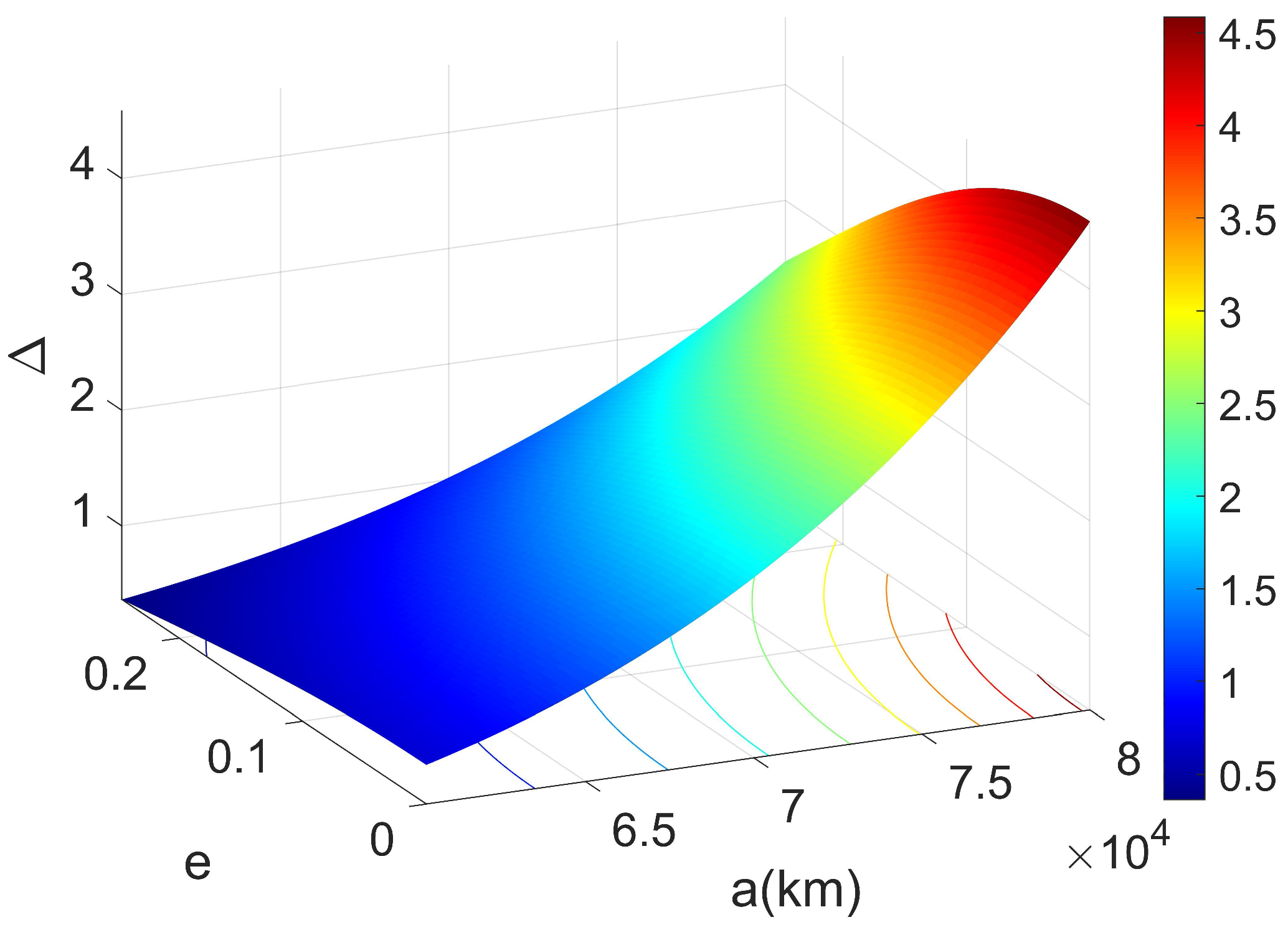
For sun-synchronous orbits, we can derive the inequality systems (5) to calculate the inclination from theoretical analysis. The following inequalities are the requirements to find the roots of $\dot{\overline{\mathsf{\Omega }}}=n_s$.

$$\left\{\begin{array}{cc}\hfill 1-R_e/a& >e\hfill \\ \hfill \frac{C^2}{4A^2}+\frac{B^3}{27A^3}& \le 0\hfill \end{array}\right.$$

(5)

The first inequality in (5) prevents the spacecraft from crashing into the outer atmosphere of Saturn. The second inequality is the discriminant of Equation (4). Then we obtain the plot of the discriminant, Figure 1.

We learn from Figure 1 that the discriminant is almost always positive for any chosen a and e. It means Equation (4) only has one real root, and there is only one sun-synchronous orbit for any chosen semimajor axis and eccentricity. Here, we choose the orbital elements $a=$ 62,268 km and $e=0.01$, substitute them into Equation (4), and solve the equation. Then the inclination $i=90.0483$ deg can be obtained naturally.

Here we continue to analyze the perturbations of spacecraft in circular sun-synchronous orbits. The spacecraft located in circular sun-synchronous orbits around Saturn would be perturbed by the Sun. The derivative of inclination is presented by using the Lagrange equations as [33,34]:

$$\begin{array}{cc}\hfill \frac{di}{dt}=& \frac{rcos(\omega +f)}{n{a}^2\sqrt{1-e^2}}{F}_n\hfill \\ \hfill \approx & \frac{3n_s^{2}cos(\omega +f)cos\xi }{n}(cos{\beta }_{s}sinisin\mathsf{\Omega }-sin{\beta }_{s}cos{i}_{s}sinicos\mathsf{\Omega }+sin{\beta }_{s}sin{i}_{s}cosi),\hfill \\ \hfill cos\xi =& cos{\beta }_s[cos(\omega +f)cos\mathsf{\Omega }-cosisin(\omega +f)sin\mathsf{\Omega }]+sin{\beta }_{s}cos{i}_s[cos(\omega +f)sin\mathsf{\Omega }\hfill \\ \hfill & +cosisin(\omega +f)cos\mathsf{\Omega }]+sin{\beta }_{s}sin{i}_{s}sinisin(\omega +f),\hfill \end{array}$$

where $F_n$ is the normal perturbation force caused by the solar gravitation, $n_s$ is the angular speed of Saturn around the Sun, ${\beta }_s$ is the ecliptic longitude of the Sun, $i_s$ is the obliquity of the ecliptic of Saturn, and $\xi$ is the angle between the unit vector from center of mass of Saturn pointing the spacecraft and the unit vector from center of mass of Saturn pointing at the Sun. Then we average the secular derivative of inclination in a period of circular sun-synchronous orbits [35]. We could see the secular inclination perturbation as:

$$\begin{array}{c}\hfill \overline{\frac{di}{dt}}=-\frac{3n_s^2}{16n}sini{(1+cos{i}_s)}^{2}sin(2{\beta }_s-2\mathsf{\Omega })\end{array}$$

(6)

It is important to emphasize that we only consider the secular effect of perturbations. We can substitute $\frac{di}{dt}$ for $\overline{\frac{di}{dt}}$ for convenience. $(2{\beta }_s-2\mathsf{\Omega })$ in Equation (6) is associated with the local time drift at the descending node.

The semimajor axis decay due to atmospheric drag leads to a shorter period and damage of the recursive feature. Here we simply assume the atmosphere of Saturn is stationary. According to the preliminary study of Saturn atmosphere model [8], we could estimate the acceleration of semi-major axis caused by atmospheric drag. We describe the variation of semimajor axis due to atmospheric drag of circular orbits by [29,36]

$$\frac{da}{dt}=-\frac{S{C}_d\rho n{a}^2}{m},$$

(7)

where $C_d$ is the drag coefficient, S is the projected area, $\rho$ is the neutral atmosphere density, and m is the mass of spacecraft.

When we analyze the inclination perturbation, we can calculate the local time drift at the descending node instead. Meanwhile, it is a fact that the local time drift at the descending node is also the local time drift at ascending node. Thus, we could continue to analyze the evolution of the ascending node. According to Equation (3), the first-order approximation of $\dot{\overline{\mathsf{\Omega }}}$ by using first-order Taylor expansion is

$$\begin{array}{cc}\hfill \mathsf{\Delta }\dot{\overline{\mathsf{\Omega }}}& =\frac{\partial \mathsf{\Delta }\dot{\overline{\mathsf{\Omega }}}}{\partial a}\mathsf{\Delta }a+\frac{\partial \mathsf{\Delta }\dot{\overline{\mathsf{\Omega }}}}{\partial i}\mathsf{\Delta }i\hfill \end{array}$$

(8)

where

$$\left\{\begin{array}{cc}\hfill \mathsf{\Delta }a& =\mathsf{\Delta }{a}_0+\frac{da}{dt}(t-t_0)\hfill \\ \hfill \mathsf{\Delta }i& =\mathsf{\Delta }{i}_0+\frac{di}{dt}(t-t_0)\hfill \end{array}\right.$$

$$\begin{array}{cc}\hfill \frac{\partial \dot{\overline{\mathsf{\Omega }}}}{\partial a}& =\frac{21n{J}_2{R}_e^{2}cosi}{4p^3}(1-e^2)+\frac{99n{J}_2^2{R}_e^4}{8p^5}(1-e^2)\{[\frac{3}{2}-\frac{5}{3}{sin}^{2}i-\frac{35J_4}{18J_2^2}(\frac{6}{7}-\frac{3}{2}{sin}^{2}i)]\hfill \\ \hfill & +[\frac{1}{6}+\frac{5}{24}{sin}^{2}i-\frac{35J_4}{18J_2^2}(\frac{9}{7}-\frac{9}{4}{sin}^{2}i)]e^2+(1-\frac{3}{2}{sin}^{2}i)\sqrt{1-e^2}\}cosi\hfill \\ \hfill \frac{\partial \dot{\overline{\mathsf{\Omega }}}}{\partial i}& =\frac{3n{J}_2{R}_e^{2}sini}{2p^2}-\frac{9n{J}_2^2{R}_e^4}{4p^4}\{[(-\frac{29}{6}+\frac{15J_4}{2J_2^2})sini+(5-\frac{35J_4}{4J_2^2}){sin}^{3}i]\hfill \\ \hfill & +[(\frac{1}{4}+\frac{45J_4}{4J_2^2})sini-(\frac{5}{8}+\frac{105J_4}{8J_2^2}){sin}^{3}i]e^2+(-4sini+\frac{9}{2}{sin}^{3}i)\sqrt{1-e^2}\}\hfill \end{array}$$

For Saturn, because the rotation period is 10.656 h, 1 deg drift of the ascending node results in $1.776$ min drift of spacecraft. Then according to Equation (8), the local time drift of spacecraft at ascending node is:

$$\begin{array}{cc}\hfill \mathsf{\Delta }T=& \frac{1.776\times 180}{\pi }\mathsf{\Delta }\mathsf{\Omega }\left(t\right)\hfill \\ \hfill =& \frac{1.776\times 180}{\pi }[\mathsf{\Delta }\mathsf{\Omega }\left(t_0\right)+\frac{\partial \dot{\overline{\mathsf{\Omega }}}}{\partial a}\mathsf{\Delta }a\left(t_0\right)(t-t_0)+\frac{1}{2}\frac{\partial \dot{\overline{\mathsf{\Omega }}}}{\partial a}\frac{da}{dt}{(t-t_0)}^2\hfill \\ \hfill & +\frac{\partial \dot{\overline{\mathsf{\Omega }}}}{\partial i}\mathsf{\Delta }i\left(t_0\right)(t-t_0)+\frac{1}{2}\frac{\partial \dot{\overline{\mathsf{\Omega }}}}{\partial i}\frac{di}{dt}{(t-t_0)}^2].\hfill \end{array}$$

(9)

The unit of spacecraft running time is second. The local time drift is counted in minutes.

When we only investigate the local time drift caused by solar gravitation, Equation (9) could be rewritten as

$$\begin{array}{cc}\hfill \mathsf{\Delta }T=& \frac{1.776\times 180}{\pi }[\mathsf{\Delta }\mathsf{\Omega }\left(t_0\right)+\frac{\partial \dot{\overline{\mathsf{\Omega }}}}{\partial a}\mathsf{\Delta }a\left(t_0\right)(t-t_0)\hfill \\ \hfill & +\frac{\partial \dot{\overline{\mathsf{\Omega }}}}{\partial i}\mathsf{\Delta }i\left(t_0\right)(t-t_0)+\frac{1}{2}\frac{\partial \dot{\overline{\mathsf{\Omega }}}}{\partial i}\frac{di}{dt}{(t-t_0)}^2].\hfill \end{array}$$

(10)

There are four initial variables, $\mathsf{\Delta }\mathsf{\Omega }\left(t_0\right)$, $\mathsf{\Delta }a\left(t_0\right)$, $\mathsf{\Delta }i\left(t_0\right)$, and $-({\beta }_s-\mathsf{\Omega })$ in Equation (10). In this paper, we assume $\mathsf{\Delta }\mathsf{\Omega }\left(t_0\right)=0$ and only consider the effect of other three variables of a given sun-synchronous orbit around Saturn.

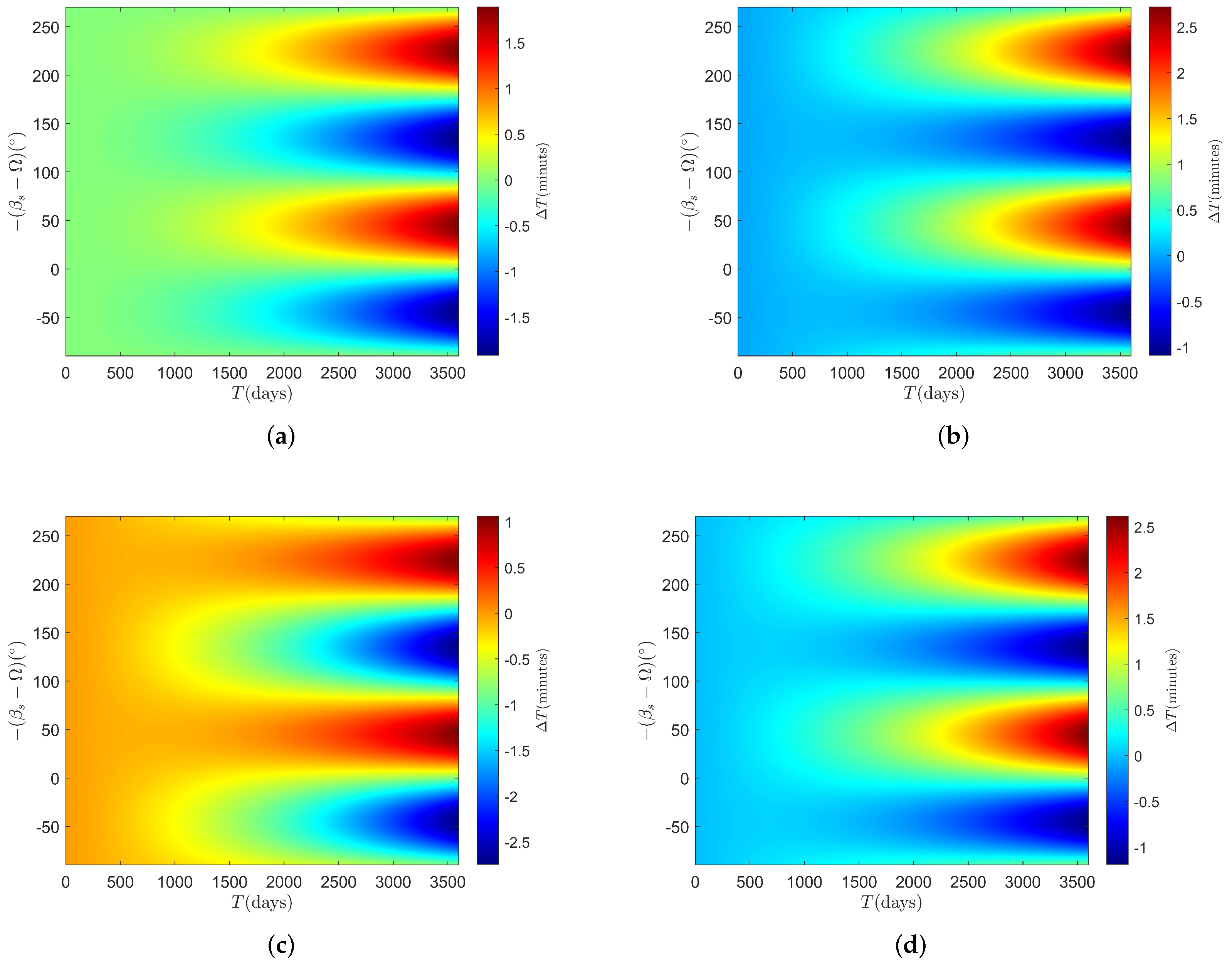
The initial orbital elements of the circular sun-synchronous orbits given in this paper are $a=$ 62,268 km$,e=0.01,i=90.0483$ deg, $\mathsf{\Omega }=-45$ deg, $\omega =30$ deg, and $M=0$ deg. The ecliptic of longitude of the Sun is fixed at ${\beta }_s=90$ deg.

When we choose small initial orbital deviation $\mathsf{\Delta }{a}_0=1$ km, $\mathsf{\Delta }{i}_0=0.001$ deg, and arbitrary $\mathsf{\Omega }\in [0,360]$ deg, we could know the local time drift at any descending node after 10 Earth years in Figure 2a. In Figure 2a, in the range of $-({\beta }_s-\mathsf{\Omega })\in [0,90]\cup [180,270]$ deg, the local time drift $\mathsf{\Delta }T$ is positive, which means the local time at descending node has been delayed. In the range $-({\beta }_s-\mathsf{\Omega })\in [90,180]\cup [-90,0]$ deg, the local time drift $\mathsf{\Delta }T$ is negative, which means the local time at the descending node has been brought forward. When the initial inclinaiton deviation is slightly greater, the local time in a larger range of $-({\beta }_s-\mathsf{\Omega })$ in Figure 2b is delayed. On the contrary, when we choose a negative initial inclination deviation, the absolute value is equal to the initial inclination deviation of Figure 2b, the local time of more area of Figure 2c is brought forward. Furthermore, we could still observe from Figure 2a–c that the distribution of the extremum of local time drift is fixed, regardless of whether and how the value and sign of $-({\beta }_s-\mathsf{\Omega })$ change. To reduce the influence of different choices of initial condition, we choose the value of $-({\beta }_s-\mathsf{\Omega })$ where the local time drift will reach the extremum after 10 Earth years. Therefore, in this paper, we fix the value $-({\beta }_s-\mathsf{\Omega })=-135$ deg, which means the local time at the descending node is 15:00.

When we fix the initial inclination deviation and choose different initial semimajor axis deviation, comparing Figure 2b with Figure 2d, the extremum of local time drift of these two figures almost have the same distribution. This means the first-order approximation of local time drift is sensitive to the initial inclination deviation and insensitive to the initial semimajor axis deviation. Thus, we fix the semimajor axis deviation in this paper $\mathsf{\Delta }{a}_0=1$ km.

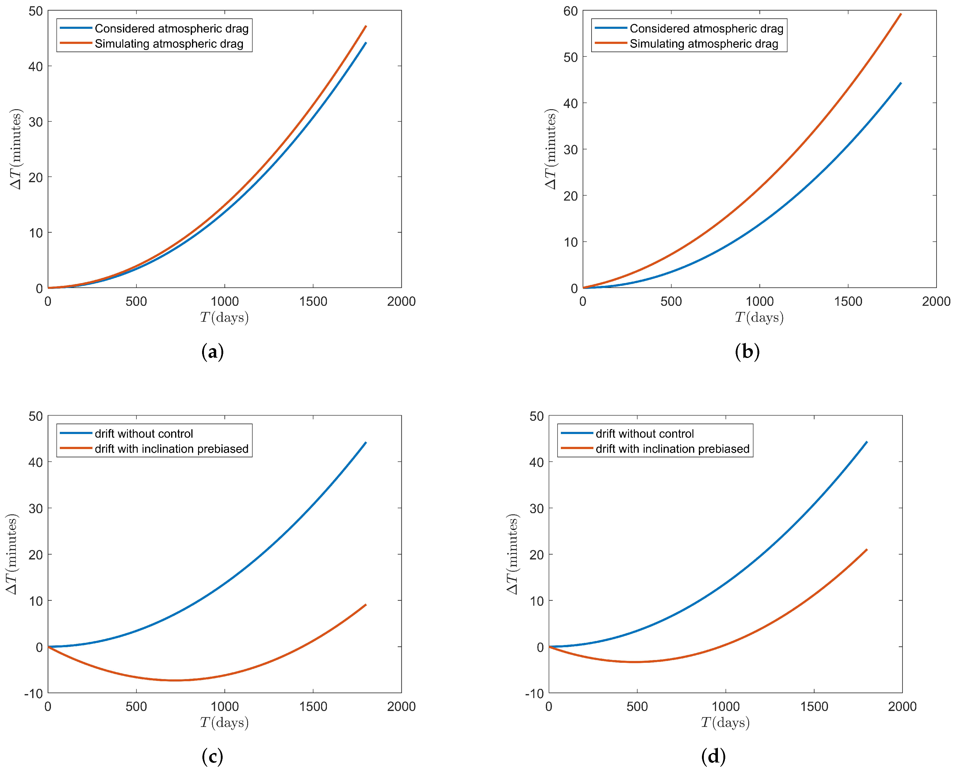
When we consider the solar gravitation perturbation and the atmospheric drag at the same time, we should use Equation (9) to calculate the local time drift at the descending node. The fact we should notice is that the changing trend of $\frac{da}{dt}$ and $\frac{di}{dt}$ is quadratic function of time t [29]. Therefore, we try to simulate the effect of atmospheric drag by using the inclinaiton drift caused by solar gravity. In this way, we only need to choose inclination prebiased methods to offset the local time drift caused by two different kinds of force. The explicit calculation of local time drift:

$$\begin{array}{cc}\hfill \mathsf{\Delta }\tilde{T}=& \frac{1.776\times 180}{\pi }\mathsf{\Delta }\mathsf{\Omega }(t)\hfill \\ \hfill =& \frac{1.776\times 180}{\pi }\{\mathsf{\Delta }\mathsf{\Omega }(t_0)+(\frac{\partial \dot{\overline{\mathsf{\Omega }}}}{\partial a}\frac{da}{dt}/\frac{\partial \dot{\overline{\mathsf{\Omega }}}}{\partial i}\frac{di}{dt}+1)\hfill \\ & [\frac{\partial \dot{\overline{\mathsf{\Omega }}}}{\partial i}\mathsf{\Delta }i(t_0)(t-t_0)+\frac{1}{2}\frac{\partial \dot{\overline{\mathsf{\Omega }}}}{\partial i}\frac{di}{dt}{(t-t_0)}^2]\}.\hfill \end{array}$$

(11)

We find two figures to test the effect of simulating method used in Equation (11). In each figure, there are two curves representing the local time drift in 5 years in different calculation methods. The curves which have considered atmospheric drag use Equation (9). The curves simulating the atmospheric drag use Equation (11). Comparing Figure 3a with Figure 3b, we learn that the circular sun-synchronous orbits with the smaller initial inclination deviation has the better simulating effect of atmospheric drag.

Then we use two methods in this paper to offset the local time drift at the descending node.

The first control strategy is using initial inclination biased method. This control strategy suits the spacecraft whose entire lifetime is not too long. We take an initial inclination bias to make the spacecraft located in a quasi-sun-synchronous orbit. Then the inclination of the quasi-sun-synchronous orbit will oscillate around its normal inclination in its lifetime but still maintain the feature of sun-synchronous orbits.

When $t_e=-\frac{\mathsf{\Delta }i\left(t_0\right)}{\frac{di}{dt}}$, the local time drift $\mathsf{\Delta }\tilde{T}$ in Equation (11) sees its extremum

$$\mathsf{\Delta }\tilde{T}\left(t_e\right)=-\frac{3996}{25\pi }\frac{\partial \dot{\overline{\mathsf{\Omega }}}}{\partial i}\frac{\mathsf{\Delta }i{\left(t_0\right)}^2}{\frac{di}{dt}}.$$

(12)

If the end of lifetime of the spacecraft is $t_f$, then the limit of local time drift at descending node is $|\mathsf{\Delta }\tilde{T}\left(tf\right)|\le \mathsf{\Delta }\tilde{T}\left(t_e\right)$. Let $\mathsf{\Delta }\tilde{T}\left(t_f\right)=-\mathsf{\Delta }\tilde{T}\left(t_e\right)$, then we find the initial inclination bias:

$$\mathsf{\Delta }i\left(t_0\right)=(1-\sqrt{2})\frac{di}{dt}{t}_f.$$

(13)

From Figure 3c,d, we learn that the prebiased initial strategy damps the local time drift at the descending node in the designed 5 Earth years’ lifetime of spacecraft.

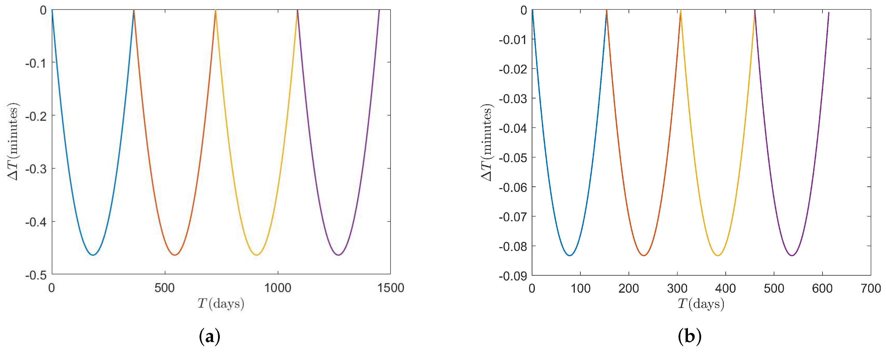
The second control strategy is designed for the spacecraft which need to execute a long-time mission. This method needs periodic inclination bias to damp the local time drift caused by solar gravitation. The extremum of local time drift Equation (11) in a period $t_c=-2\frac{\mathsf{\Delta }i\left(t_{c_0}\right)}{\frac{di}{dt}}$ is equal to a fixed local time drift limitation $\mathsf{\Delta }\tilde{T}$

$$|\mathsf{\Delta }\tilde{T}\left(\frac{t_c}{2}\right)|=|\mathsf{\Delta }\tilde{T}|,$$

use the calculation equation in

$$\begin{array}{c}\hfill \frac{1.776\times 180}{\pi }[\mathsf{\Delta }\mathsf{\Omega }(t_0)-\frac{1}{2}(\frac{\partial \dot{\overline{\mathsf{\Omega }}}}{\partial a}\frac{da}{dt}/\frac{\partial \dot{\overline{\mathsf{\Omega }}}}{\partial i}\frac{di}{dt}+1)\frac{\partial \dot{\overline{\mathsf{\Omega }}}}{\partial i}\frac{\mathsf{\Delta }i{(t_{c_0})}^2}{\frac{di}{dt}}]=\left|\mathsf{\Delta }\tilde{T}\right|\end{array}$$

when $\mathsf{\Delta }\mathsf{\Omega }(t_0)=0$, then we find

$$\begin{array}{c}\hfill -\frac{3996}{25\pi }(\frac{\partial \dot{\overline{\mathsf{\Omega }}}}{\partial a}\frac{da}{dt}/\frac{\partial \dot{\overline{\mathsf{\Omega }}}}{\partial i}\frac{di}{dt}+1)\frac{\partial \dot{\overline{\mathsf{\Omega }}}}{\partial i}\frac{\mathsf{\Delta }i{(t_{c_0})}^2}{\frac{di}{dt}}=\left|\mathsf{\Delta }\tilde{T}\right|\end{array}$$

and the value of periodic inclination bias can be derived naturally:

$$|\mathsf{\Delta }i\left(t_{c_0}\right)|=\sqrt{|\frac{25\pi }{3996}\frac{\frac{di}{dt}\mathsf{\Delta }\tilde{T}}{\frac{\partial \dot{\overline{\mathsf{\Omega }}}}{\partial i}(\frac{\partial \dot{\overline{\mathsf{\Omega }}}}{\partial a}\frac{da}{dt}/\frac{\partial \dot{\overline{\mathsf{\Omega }}}}{\partial i}\frac{di}{dt}+1)}|}$$

(14)

where the sign of $\mathsf{\Delta }i\left(t_{c_0}\right)$ is opposite to the sign of $\frac{di}{dt}$.

From Figure 3c,d, compared with Figure 4a,b, the periodic inclination biased method has the better effect of local time drift limitation. Meanwhile, comparing Figure 4a with Figure 4b, it is obviously also sensitive to the initial inclination deviation. Therefore, regardless of the methods, it is essential to limit the initial inclination deviation $\mathsf{\Delta }{i}_0$.

3. Repeating Ground Track Orbits and Orbital Maintenance

The repeating ground track is significant for remote sensing satellites. The condition for spacecraft achieving repeating ground track is $R\mathsf{\Delta }\lambda =2\pi N$, where R and N are relatively positive prime numbers. The interval of the adjacent ground track on the equator is [28,29]

$$\mathsf{\Delta }\lambda =T_N({\omega }_S-\dot{\overline{\mathsf{\Omega }}}),$$

(15)

which ${\omega }_S$ is the angular rotational velocity of Saturn.

The nodal period of the motion of spacecraft is

$$T_N=\frac{2\pi }{\dot{\overline{M}}+\dot{\overline{\omega }}}.$$

(16)

According to the mean element theory [16], the average perturbing rates of M and $\omega$ is [37]

$$\begin{array}{cc}\hfill \dot{\overline{M}}& =n+{\dot{M}}_1+{\dot{M}}_2,\hfill \\ \hfill \dot{\overline{\omega }}& ={\dot{\omega }}_1+{\dot{\omega }}_2,\hfill \end{array}$$

(17)

where

$$\begin{array}{cc}\hfill {\dot{M}}_1& =\frac{3n{J}_2{R}_e^2}{2p^2}(1-\frac{3}{2}{sin}^{2}i)\sqrt{1-e^2},\hfill \\ \hfill {\dot{\omega }}_1& =-\frac{3n{J}_2{R}_e^2}{2p^2}(\frac{5}{2}{sin}^{2}i-2),\hfill \end{array}$$

(18)

$$\begin{array}{cc}\hfill {\dot{M}}_2& =\frac{9n{J}_2^2{R}_e^4}{8p^4}(1-e^2){(1-\frac{3}{2}{sin}^{2}i)}^2\hfill \\ \hfill & +\frac{9n{J}_2^2{R}_e^4}{4p^4}\{\sqrt{1-e^2}(\frac{5}{2}-\frac{19}{3}{sin}^{2}i+\frac{233}{48}{sin}^{4}i)\hfill \\ \hfill & +\frac{e^4}{\sqrt{1-e^2}}(\frac{35}{12}-\frac{35}{4}{sin}^{2}i+\frac{315}{32}{sin}^{4}i)\hfill \\ \hfill & +\sqrt{1-e^2}{e}^2[(\frac{10}{3}-\frac{5J_4}{4J_2^2})+(-\frac{26}{3}+\frac{25J_4}{4J_2^2}){sin}^{2}i+(\frac{103}{12}-\frac{175J_4}{32J_2^2}){sin}^{4}i]\},\hfill \end{array}$$

(19)

$$\begin{array}{cc}\hfill {\dot{\omega }}_2& =\frac{9n{J}_2^2{R}_e^4}{4p^4}\{(4-\frac{10J_4}{3J_2^2})+(-\frac{103}{12}+\frac{155J_4}{12J_2^2}){sin}^{2}i+(\frac{215}{48}-\frac{245J_4}{24J_2^2}){sin}^{4}i\hfill \\ \hfill & +\sqrt{1-e^2}(2-\frac{11}{2}{sin}^{2}i+\frac{15}{4}{sin}^{4}i)+e^2[(\frac{7}{12}-\frac{15J_4}{4J_2^2})+(-\frac{3}{8}+\frac{105J_4}{8J_2^2}){sin}^{2}i\hfill \\ \hfill & +(-\frac{15}{32}-\frac{315J_4}{32J_2^2}){sin}^{4}i]\}.\hfill \end{array}$$

(20)

In this paper, we use the ground track repetition parameter $Q=R/N$ to describe different repeating ground track orbits. Here, we should pay attention to the meaningful range of repetition parameter Q [29].

To find a suitable repetition parameter, we should firstly find the lower bound of Q by using the discriminant of $f(sini)$:

$$f(sini)=A_1{sin}^{4}i+B_1{sin}^{2}i+C_1=0,$$

(21)

where

$$\begin{array}{cc}\hfill A_1=& \frac{9n{J}_2^2{R}_e^4}{4p^4}[(\frac{215}{48}-\frac{15}{32}{e}^2+\frac{15}{4}\sqrt{1-e^2})-\frac{35J_4}{18J_2^2}(\frac{21}{4}+\frac{81}{16}{e}^2)]+\frac{9n{J}_2^2{R}_e^4}{4p^4}\sqrt{1-e^2}(\frac{9}{8}\sqrt{1-e^2}\hfill \\ \hfill & +\frac{233}{48}+\frac{103}{12}{e}^2+\frac{315}{32}\frac{e^4}{1-e^2}-\frac{105J_4}{32J_2^2}{e}^2),\hfill \end{array}$$

$$\begin{array}{cc}\hfill B_1& =\frac{3n{J}_2{R}_e^2}{4p^2}\{-5+\frac{3J_2{R}_e^2}{p^2}[-\frac{103}{12}-\frac{3}{8}{e}^2-\frac{11}{2}\sqrt{1-e^2}+\frac{35J_4}{6J_2^2}(\frac{31}{14}+\frac{9}{4}{e}^2)]\}-\frac{9n{J}_2{R}_e^2}{4p^2}\sqrt{1-e^2}\hfill \\ \hfill & +\frac{9n{J}_2^2{R}_e^4}{4p^4}\sqrt{1-e^2}(-\frac{3}{2}\sqrt{1-e^2}-\frac{19}{3}-\frac{26}{3}{e}^2-\frac{35}{4}\frac{e^4}{1-e^2}+\frac{25J_4}{4J_2^2}{e}^2),\hfill \end{array}$$

$$\begin{array}{cc}\hfill C_1& =\frac{3n{J}_2{R}_e^2}{4p^2}\{4+\frac{3J_2{R}_e^2}{p^2}[(4+\frac{7}{12}{e}^2+2\sqrt{1-e^2})-\frac{5J_4}{6J_2^2}(4+\frac{9}{2}{e}^2)]\}+\frac{3n{J}_2{R}_e^2}{2p^2}\sqrt{1-e^2}\hfill \\ \hfill & +\frac{9n{J}_2{R}_e^4}{4p^4}\sqrt{1-e^2}(\frac{1}{2}\sqrt{1-e^2}+\frac{5}{2}+\frac{10}{3}{e}^2+\frac{35}{12}\frac{e^4}{1-e^2}-\frac{5J_4}{4J_2^2}{e}^2)+n+Q(n_s-{\omega }_s).\hfill \end{array}$$

To promise $f(sini)$ has four real roots, the discriminant should be non-negative, i.e.,

$$B_1^2-4A_1[\widetilde{C_1}-Q({\omega }_s-n_s)]\ge 0.$$

Solving the inequality, we find the lower bound of Q:

$$Q\ge \frac{\widetilde{C_1}-\frac{B_1^2}{4A_1}}{{\omega }_s-n_s},$$

where $\widetilde{C_1}=C_1-Q(n_s-{\omega }_s)$.

To estimate the maximum of repetition parameter, we use the rotational period of Saturn $T_s$ and the period of spacecraft in a low orbit $T_l$. Then the upper bound of Q can be presented as:

$$Q\le \frac{T_s}{T_l}.$$

Using the data from the planet model of Saturn, we find the meaningful range of repetition parameter for engineering application: $2.4701\le Q\le 2.5191$.

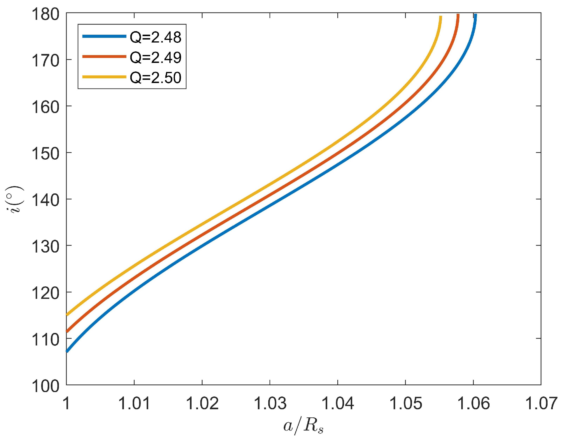
For different chosen values of repetition parameter Q, we see a function $f(sini)$ that describes the relation between the inclination i and the semimajor axis a of repeating ground track orbits. The relation between i and a are shown in Figure 5 for three given meaningful values of Q. Using Equation (21), when initial semimajor axis and eccentricity are given, the corresponding inclination is the root of $f(sini)$. 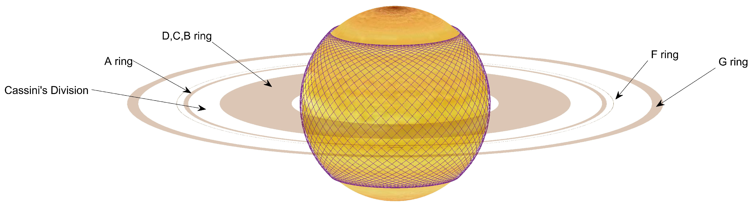In Figure 6, we present the repeating ground track orbit around Saturn when initial orbital elements and repetition parameter Q are given.

An inevitable perturbation which can cause the semimajor decay in repeating ground track orbits is atmospheric drag. The semimajor axis decay due to atmospheric drag leads to a shorter period and damage of the recursive feature.

The difference between actual angular velocity and nominal angular velocity can be presented as [29]:

$$\begin{array}{c}\hfill \mathsf{\Delta }n=-\frac{3\overline{n}}{2\overline{a}}(a_0+\frac{da}{dt}t-\overline{a}),\end{array}$$

where $a_0$ is the initial semimajor axis, $\overline{a}$ is the nominal semimajor axis, and $\overline{n}$ is nominal angular speed.

The increase in angular speed results in the longitude drift of ground track. Obviously, we can learn from Equation (7) that $\dot{a}<0$. Therefore, if $a_0\le \overline{a}$, the longitude will drift eastward monotonously. To maintain the feature of repeating ground track orbits, we should take a maneuver to make initial semimajor axis $a_0>\overline{a}$. Then, in the first coming time interval $t_s=-\frac{\mathsf{\Delta }a}{\dot{a}}$, the longitude will drift westward. When $\frac{d\mathsf{\Delta }\lambda }{dt}=-\frac{3\pi }{\overline{a}}(\mathsf{\Delta }a+\dot{a}t)=0$, the longitude of the ground track would reach the western boundary. In the second time interval $t_s$, the longitude will drift eastward and finally return back to the initial longitude. Then we can find the longitude drift compared to the nominal repeating ground track orbits:

$$\begin{array}{cc}\hfill \mathsf{\Delta }\lambda & =-\frac{{\omega }_s}{\overline{n}}{\int }_0^t\frac{3\overline{n}}{2\overline{a}}(a_0+\frac{da}{dt}t-\overline{a})dt\hfill \\ \hfill & =-\frac{3{\omega }_s}{2\overline{a}}[(a_0-\overline{a})t+\frac{1}{2}\dot{a}{t}^2],\hfill \end{array}$$

(22)

where ${\omega }_s$ is the angular rotation speed of Saturnian.

In the whole control period, when we fix the limitation of longitude drift $\mathsf{\Delta }{\lambda }_L$, then we can find the control period $\mathsf{\Delta }{T}_C$ and compensation $\mathsf{\Delta }a$ of semimajor axis [29]:

$$\begin{array}{cc}\hfill & \mathsf{\Delta }{\lambda }_L=-\frac{3\pi {\left(\mathsf{\Delta }a\right)}^2}{2\overline{a}\dot{a}},\hfill \\ \hfill & \mathsf{\Delta }a=\sqrt{-\frac{2\overline{a}\dot{a}\mathsf{\Delta }\lambda }{3\pi }},\hfill \\ \hfill & \mathsf{\Delta }{T}_C=-\frac{2\mathsf{\Delta }a}{\dot{a}}.\hfill \end{array}$$

(23)

Thus, in each period, when the longitude of ground track drift to the eastern boundary, we have to take a maneuver $\mathsf{\Delta }a$ to compensate the decay of semimajor axis. Here we assumed projected area of spacecraft $S=20{\mathrm{m}}^2$, $C_d=2.1$, $\mathsf{\Delta }{\lambda }_L=10$ km, and mass $m=3000$ kg. The density of simplified atmospheric model, in the range of semi-major axis $a\in [$62,268, 62,468] km, is $\rho \in [3.7\times {10}^{-12},4.7\times {10}^{-12}]$ kg$/{\mathrm{m}}^3$ [8]. 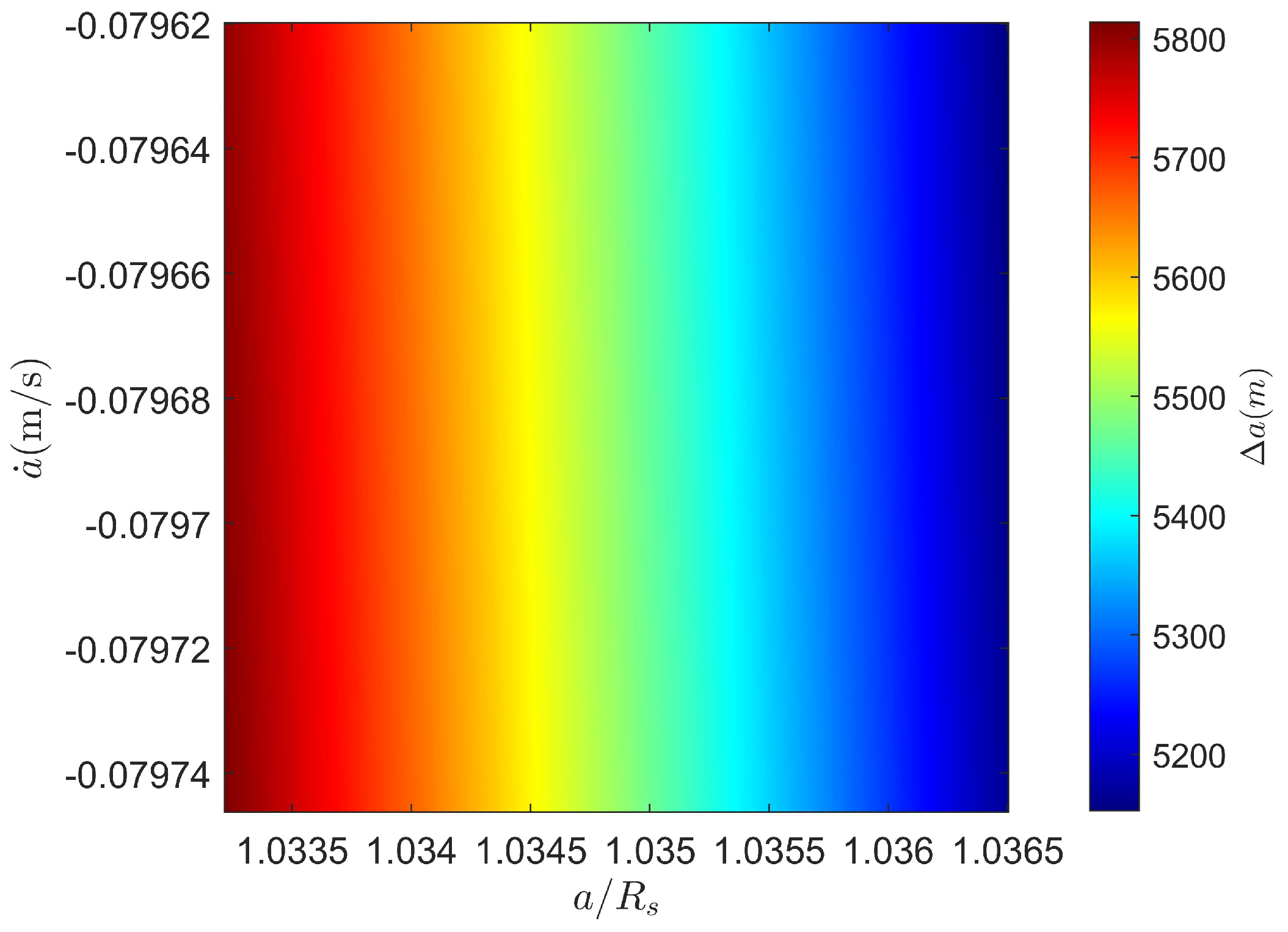Then we find the Figure 7 and Figure 8 which illustrate the the control compensation of semimajor axis and control period of repeating ground track orbits. From Figure 7, we know the semimajor compensation $\mathsf{\Delta }a$ for $a\in [$62,268, 62,468] km varies from 5200 m to 5800 m. The corresponding compensation period $\mathsf{\Delta }{T}_C$ in Figure 8 varies from 18 h to 16 h. Compared to Jupiter [29], Saturnian atmospheric drag is about 2 orders of magnitude greater than Jovian atmospheric drag when the spacecraft is at the same altitude. As a result, it is essential to execute the semimajor axis compensation for repeating ground track orbits around Saturn.

4. Frozen Orbits

Before analyzing frozen orbits, we first investigate the orbits at the critical inclination. The traditional design of the orbits at critical inclination around Earth just considers the $J_2$ term by which the first order secular variation of eccentricity and argument of perigee are [15,16]:

$$\begin{array}{cc}\hfill {\dot{e}}_1& =0,\hfill \\ \hfill {\dot{\omega }}_1& =-\frac{3n{J}_2{R}_2^2}{2a^2{(1-e^2)}^2}(\frac{5}{2}{sin}^{2}i-2).\hfill \end{array}$$

Different from the methods which only considered $J_2$, we still need to calculate the perturbation caused by $J_2$ and $J_4$ terms. Though the magnitude of $J_2$ term exceeds $J_3$ term 1000 times, $J_4$ term still plays an important role in aspheric perturbation. Thus, the conditions for the orbits at the critical inclination should be combined ${\omega }_1$ with ${\omega }_2$:

$$\begin{array}{cc}\hfill & {\dot{e}}_1={\dot{e}}_2=0,\hfill \\ \hfill & \dot{\overline{\omega }}={\dot{\omega }}_1+{\dot{\omega }}_2=0.\hfill \end{array}$$

(24)

However, the critical inclination cannot satisfy most missions for remote sensing satellites. For the purpose of missions, we must consider the frozen orbits around Saturn. Frozen orbits are the orbits which own small constant eccentricity and constant argument of perigee while arbitrary inclination and orbiting altitude can be chosen. The frozen orbits we designed which have small eccentricity must consider first order long-period terms [23]. The main parts of long-period terms are [16]

$$\begin{array}{cc}\hfill {\dot{e}}_1^l& =-\frac{J_3{R}_e}{2J_{2}p}sini(1-e^2)sin\omega ,\hfill \\ \hfill {\dot{\omega }}_1^l& =-\frac{J_3{R}_e}{2e{J}_{2}p}(1-\frac{e^2{cos}^{2}i}{sini})cos\omega .\hfill \end{array}$$

(25)

Then the complete conditions for frozen orbits are combined by Equations (24) and (25) [23].

$$\left\{\begin{array}{cc}\hfill \dot{\overline{e}}& ={\dot{e}}_1+{\dot{e}}_2+{\dot{e}}_1^l=0,\hfill \\ \hfill \dot{\overline{\omega }}& ={\dot{\omega }}_1+{\dot{\omega }}_2+{\dot{\omega }}_1^l=0.\hfill \end{array}\right.$$

(26)

Using $\omega ={90}^{\circ }$ or $\omega ={270}^{\circ }$ to solve Equation (26), respectively, we learn that only when $\omega ={270}^{\circ }$ can the eccentricity e be positive. In Figure 9, the values of eccentricity are presented for different combinations of semimajor axis and inclianition.

5. Stationary Orbits and Orbital Maintenance

Stationary orbits are more complex than those we have considered before. Therefore, we investigate stationary orbits in a special condition. When we investigate the stationary orbits around terrestrial planets, we must take the $J_{22}$ term into our gravitational field model and analyze the longitude drift caused by aspheric perturbation. Here we only analyze aspheric perturbation caused by the $J_2$, $J_4$ terms, as Saturn is exactly a gaseous planet which means the $J_{22}$ term could be neglected.

The spherical coordinates $O-r,\lambda ,\phi$, where O is the centroid of Saturn, r is the distant from the spacecraft instant position to O, $\lambda$ and $\phi$ represent the longitude and latitude of the spacecraft separately. The equations of motion of stationary orbits in the spherical coordinates can be written as [28]

$$\left\{\begin{array}{cc}\hfill \ddot{r}-r{cos}^2\phi {\dot{\lambda }}^2-r{\dot{\phi }}^2=& -\frac{\mu }{r^2}-\frac{3\mu J_2{R}_e^2}{2r^4}(3{sin}^2\phi -1)\hfill \\ \hfill & +\frac{5\mu J_4{R}_e^4}{8r^6}(35{sin}^4\phi -30{sin}^2\phi +3),\hfill \\ \hfill \frac{d}{dt}\left(r^2\dot{\lambda }{cos}^2\phi \right)=& 0,\hfill \\ \hfill r\ddot{\phi }+2\dot{r}\dot{\phi }+\frac{1}{2}{r}^{2}sin\left(2\phi \right){\dot{\lambda }}^2=& -[\frac{3\mu J_2{R}^2}{2r^3}+\frac{\mu J_4{R}^4}{8r^5}(70{sin}^2\phi -30)]sin2\phi .\hfill \end{array}\right.$$

(27)

Spacecraft staying in stationary orbits around Saturn must satisfy these conditions [28]:

$$\left\{\begin{array}{cc}\hfill \dot{r}& =\ddot{r}=0,\hfill \\ \hfill \dot{\lambda }& =n,\ddot{\lambda }=0,\hfill \\ \hfill \dot{\phi }& =\ddot{\phi }=0.\hfill \end{array}\right.$$

Then we gain the equation of stationary orbits at $\phi =0$ as

$$\frac{\mu }{r^3}+\frac{3\mu J_2{R}^2}{2r^5}-\frac{15\mu J_4{R}^4}{8r^7}=n^2.$$

(28)

Solving Equation (28), we find the radius of stationary orbits around Saturn is $r_s$ = 112,506.0294 km.

After learning the structure of Saturn’s rings [12], we know that spacecraft in the stationary orbit around Saturn may have a collision with the B-ring.

Using nonsingular elements $\{a,e_x=ecos(\mathsf{\Omega }+\omega ),e_y=esin(\mathsf{\Omega }+\omega )$, $i_x=sinisin\mathsf{\Omega }$, $i_y=sinicos\mathsf{\Omega }$, $\lambda =\mathsf{\Omega }+\omega +M\}$, we first calculate the secular solar gravitation perturbation of $i_x,i_y$ and $e_x,e_y$. When $\phi =0$, the normal perturbation force caused by the solar gravitation can be written as [33]:

$$F_n=3r{n}_s^2(sin\alpha sin{\beta }_{s}cos{i}_s+cos\alpha cos{\beta }_s)sin{\beta }_{s}sin{i}_s,$$

(29)

where $\alpha$ is the longitude of spacecraft in the stationary orbit, $n_s$ is the angular speed of Saturn around the Sun, ${\beta }_s$ is the ecliptic longitude of the Sun, $i_s$ is the obliquity of the ecliptic of Saturn. The derivative of $i_x,i_y$ perturbed by normal solar gravitation in a Saturnian rotation period are [33]

$$\begin{array}{cc}\hfill \frac{d{i}_x}{dt}=& \frac{3n_s^2}{n}[\frac{1}{4}{sin}^2{\beta }_{s}sin2i_s+(\frac{1}{8}sin2{\beta }_{s}cos{i}_s)i_x,\hfill \\ \hfill & +(-\frac{1}{8}{cos}^2{\beta }_s-\frac{3}{8}{sin}^2{\beta }_{s}cos{i}_s+\frac{1}{2}sin{\beta }_{s}sin{i}_s)i_y],\hfill \end{array}$$

(30)

$$\begin{array}{cc}\hfill \frac{d{i}_y}{dt}=& \frac{3n_s^2}{n}[\frac{1}{4}sin2{\beta }_{s}sin{i}_s-(\frac{1}{8}sin2{\beta }_{s}cos{i}_s)i_x\hfill \\ \hfill & +(\frac{1}{8}{cos}^2{\beta }_s+\frac{3}{8}{sin}^2{\beta }_{s}cos{i}_s-\frac{1}{2}sin{\beta }_{s}sin{i}_s)i_y].\hfill \end{array}$$

(31)

Here, we apply the Equations (30) and (31) to analyze the perturbation of the stationary orbit caused by solar gravitation, then we find the average rate of inclination vector perturbed by solar gravity in a sidereal orbit period:

$$\left\{\begin{array}{cc}\hfill \frac{\mathsf{\Delta }{i}_x}{\mathsf{\Delta }t}=& \frac{1}{2\pi }{\int }_0^{2\pi }\frac{d{i}_x}{dt}d{\beta }_s\hfill \\ \hfill =& \frac{3n_s^2}{n}[(-\frac{1}{16}-\frac{3}{16}{cos}^2{i}_s+\frac{1}{4}{sin}^2{i}_s)i_y+\frac{1}{4}sin{i}_{s}cos{i}_s],\hfill \\ \hfill \frac{\mathsf{\Delta }{i}_y}{\mathsf{\Delta }t}=& \frac{1}{2\pi }{\int }_0^{2\pi }\frac{d{i}_y}{dt}d{\beta }_s\hfill \\ \hfill =& \frac{3n_s^2}{n}(\frac{1}{16}+\frac{3}{16}{cos}^2{i}_s-\frac{1}{4}{sin}^2{i}_s)i_x.\hfill \end{array}\right.$$

(32)

After solving this first order linear ordinary differential equation system Equation (32), we find the $i_x(t),i_y(t)$ for any time t with initial condition $i_x(t_0),i_y(t_0)$.

$$\begin{array}{cc}\hfill i_x(t)=& i_x(t_0)cos[\frac{3n_s^2}{32n}(7cos(2i_s)+1)t]\hfill \\ \hfill & -(i_y(t_0)-\frac{4sin(2i_s)}{7cos(2i_s)+1})sin[\frac{3n_s^2}{32n}(7cos(2i_s)+1)t]\hfill \\ \hfill =& (0.621896-i_y(t_0))sin(1.35686\times {10}^{-13}t)+i_x(t_0)cos(1.35686\times {10}^{-13}t),\hfill \\ \hfill i_y(t)=& i_x(t_0)sin[\frac{3n_s^2}{32n}(7cos(2i_s)+1)t]\hfill \\ \hfill & +(i_y(t_0)-\frac{4sin(2i_s)}{7cos(2i_s)+1})cos[\frac{3n_s^2}{32n}(7cos(2i_s)+1)t]+\frac{4sin(2i_s)}{7cos(2i_s)+1}\hfill \\ \hfill =& 0.621896+i_x(t_0)sin(1.35686\times {10}^{-13}t)\hfill \\ \hfill & +(i_y(t_0)-0.621896)cos(1.35686\times {10}^{-13}t).\hfill \end{array}$$

(33)

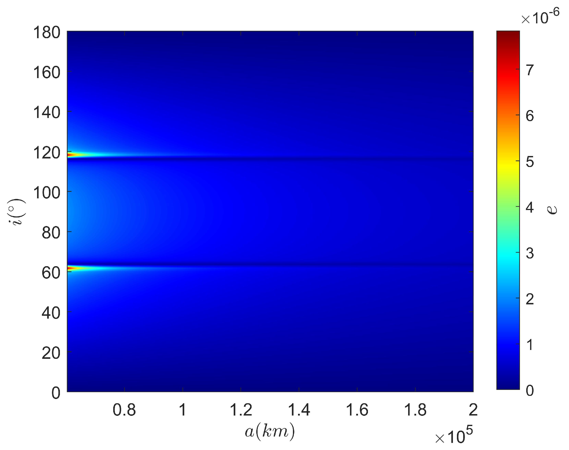
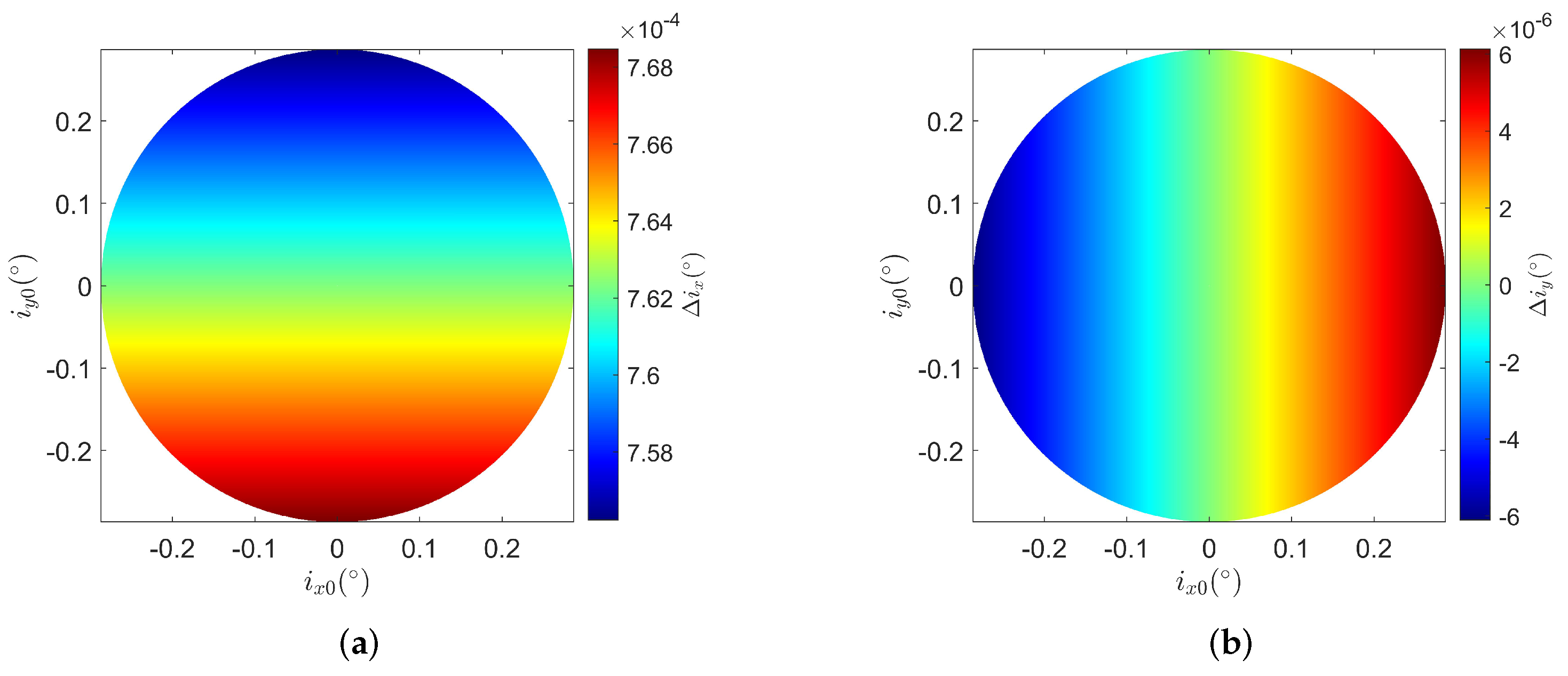
Before we analyze the perturbation of inclination vector, we firstly set the maximum of inclination perturbation $|\mathsf{\Delta }{i}_{max}|=0.{2865}^{\circ }$. Then we could draw the Figure 10a,b of $i_x,i_y$ separately for each initial condition value $i_{x_0}=i_x\left(t_0\right),i_{y_0}=i_y\left(t_0\right)$ in the limited circle. Once we see Figure 10a,b, what we know immediately is that the inclination perturbation is so small that the magnitude is smaller than $1\times {10}^{-3}$ in 5 Earth years. Furthermore, comparing Figure 10a with Figure 10b, we learn evidently that the magnitude of $\mathsf{\Delta }{i}_y$ is two order magnitude smaller than $\mathsf{\Delta }{i}_x$ in a given time of 5 Earth years. This means when we plot the perturbation of inclination vector of stationary orbit around Saturn over a long time, we could hardly see a sight difference in $i_y$.

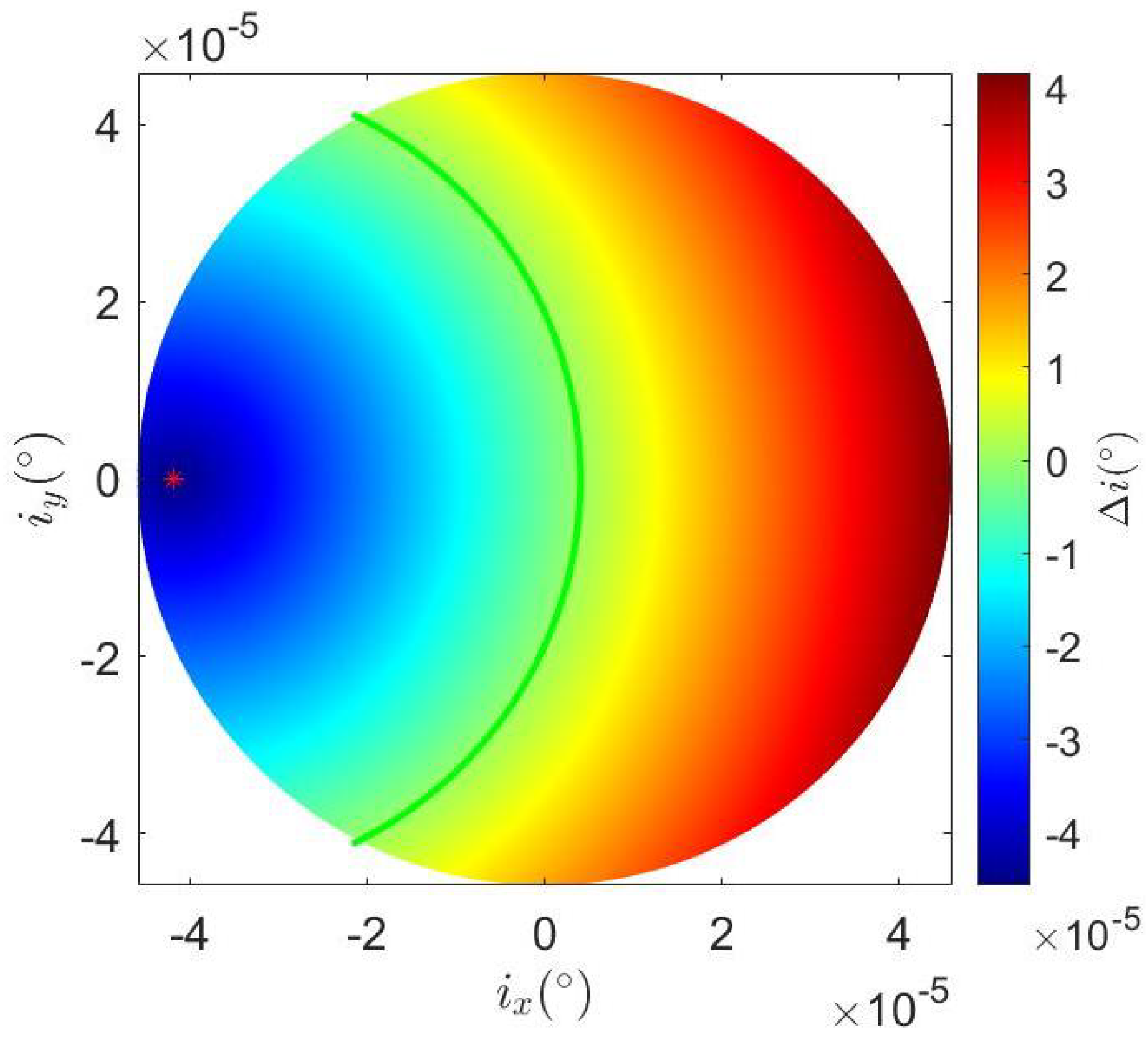
Though the inclination perturbation caused by solar gravity could hardly influence the spacecraft in stationary orbit around Saturn, we still analyze the control strategy of $i_x,i_y$ in a preliminary way. When we know how the solar gravity perturbation acts, we could calculate $\mathsf{\Delta }i$ for any initial $(i_{x_0},i_{y_0})$ to stay in the limited circle. The area of the cool tone circle overlap limited circle in Figure 11 indicates the initial point $(i_{x_0},i_{y_0})$ in this area are still remained in the limited circle after 100 Earth days. By observing the perturbation feature of stationary orbit around Saturn, we know that minimum maneuver $\overrightarrow{\mathsf{\Delta }i}$ to keep $i_x,i_y$ staying in the limited circle is from the boundary of limited circle pointing towards the center of the cool tone circle. The value of $\overrightarrow{\mathsf{\Delta }i}$ of $(i_{x_0},i_{y_0})$ in warm tone area in Figure 11 indicates the minimum inclination maneuver of $(i_{x_0},i_{y_0})$ to keep $(i_x\left(t\right),i_y\left(t\right))$ remained in the limited circle after 100 Earth days.

After analyzing the effect caused by solar gravity perturbation, we now turn to the solar radiation pressure which may lead to eccentricity drift. First, the mean solar irradiance around Saturn is $P=15.04$ W/${\mathrm{m}}^2$ while the distance from the Sun to Saturn is $1.426\times {10}^{12}$ m [38]. Then we find the intensity of solar radiation pressure is $p=\frac{P}{c}=5.0168\times {10}^{-8}$ N/${\mathrm{m}}^2$, where $c=$ 299,792,458 m/s is the speed of light. Using other supposed parameters: the reflection parameter $K=1$, area of spacecraft vertical to the Sun $A=20$ m${}^2$, the mass of spacecraft $m=3000$ kg, then the solar radiation pressure of spacecraft on stationary orbits around Saturn is [34]:

$$\begin{array}{cc}\hfill {\mathbf{F}}_{\mathbf{s}}=& -Kp\left(\frac{A}{m}\right)\mathbf{S}=3.3445\times {10}^{-10}\mathbf{S}\hfill \end{array}$$

(34)

where $\mathbf{S}$ is the unit vector from the centroid of Saturn pointing at the Sun.

Using the Lagrange perturbation equations, we could find the average time derivatives of the eccentricity vector $e_x=ecos(\omega +\mathsf{\Omega }),e_y=esin(\omega +\mathsf{\Omega })$ in Equation (35).

$$\begin{array}{cc}\hfill \frac{d{e}_x}{dt}& =\frac{1}{2\pi }{\int }_0^{2\pi }\frac{1}{na}(F_{r}sinl+2F_{t}cosl)dl\hfill \\ \hfill & =-\frac{3F_s}{2na}sin{l}_{s}cos{i}_s,\hfill \\ \hfill \frac{d{e}_y}{dt}& =\frac{1}{2\pi }{\int }_0^{2\pi }\frac{1}{na}(-F_{r}cosl+2F_{t}sinl)dl\hfill \\ \hfill & =\frac{3F_s}{2na}cos{l}_s,\hfill \end{array}$$

(35)

$$\begin{array}{cc}\hfill F_r=& -\frac{F_s}{2}[(1-cos{i}_s)cos(\mathsf{\Omega }+\omega +f+l_s)+(1+cos{i}_s)cos(\mathsf{\Omega }+\omega +f-l_s)],\hfill \\ \hfill F_t=& \frac{F_s}{2}[(1-cos{i}_s)sin(\mathsf{\Omega }+\omega +f+l_s)+(1+cos{i}_s)sin(\mathsf{\Omega }+\omega +f-l_s)].\hfill \end{array}$$

(36)

where $F_r$ and $F_t$ are the radial component and tangential component of solar radiation pressure ${\mathbf{F}}_{\mathbf{s}}$.

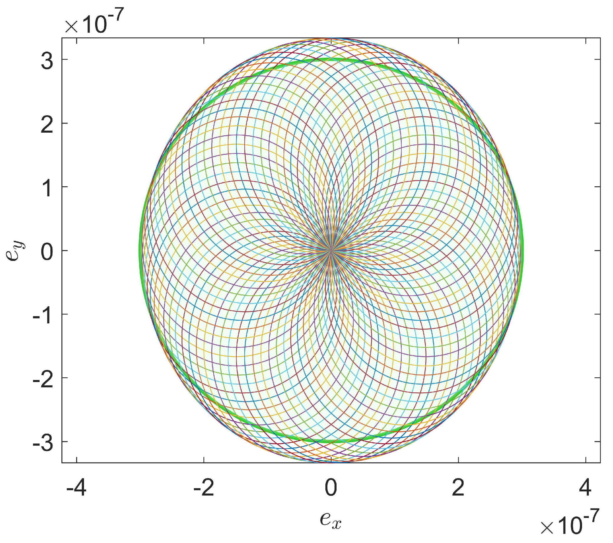
When we analyze the eccentricity perturbation of spacecraft in stationary orbits over a long time period, we learn that the motion of the Sun in a time period could be described as $\mathsf{\Delta }{l}_s=l_s\left(t\right)-l_s\left(t_0\right)=n_s(t-t_0)$. Then we find the time integral of the eccentricity vector for any given t.

$$\begin{array}{cc}\hfill e_x\left(t\right)& =e_x\left(t_0\right)+\frac{3F_s}{2na}\frac{1}{n_s}[cos{l}_s\left(t\right)-cos{l}_s\left(t_0\right)]cos{i}_s,\hfill \\ \hfill e_y\left(t\right)& =e_y\left(t_0\right)+\frac{3F_s}{2na}\frac{1}{n_s}[sin{l}_s\left(t\right)-sin{l}_s\left(t_0\right)].\hfill \end{array}$$

(37)

We learn from Equation (37) that the curve of the eccentricity vector is an ellipse due to the existence of $cos{i}_s$, and initial condition $(e_{x_0},e_{y_0})$ and $l_{s_0}$ influence the position of this eccentricity ellipse. From Figure 12, we learn that $l_{s_0}$, which means the angular between initial solar radiation direction and x axis, can influence the perturbing direction. The centre of eccentricity limitation circle is $(e_{x_0},e_{y_0})$.

Here, we fix the $(e_{x_0},e_{y_0})=(0,0)$. When $(e_{x_0},e_{y_0})\ne (0,0)$, we can first take a maneuver to make the point $(e_{x_0},e_{y_0})=(0,0)$ in the curve of eccentricity perturbation. Then, we can design a maintenance strategy. When taking an eccentricity control, we used to set $\mathsf{\Delta }{V}_t>0$, then we could suppose $B=-\frac{\mathsf{\Delta }{V}_t}{T}$, and find the maneuver function [39]:

$$\begin{array}{c}\hfill \frac{d{e}_x}{dt}=-\frac{2}{na}Bcos(l_s-\frac{\pi }{2}),\\ \hfill \frac{d{e}_y}{dt}=-\frac{2}{na}Bsin(l_s-\frac{\pi }{2}).\end{array}$$

Combined with solar radiation pressure perturbation Equation (35), the rate of eccentricity vector $(e_x,e_y)$ after a maneuver could be rewritten as

$$\begin{array}{cc}\hfill \frac{d{e}_x}{dt}& =-\frac{3F_s}{2na}sin{l}_{s}cos{i}_s+\frac{2}{na}Bcos(l_s-\frac{\pi }{2})\hfill \\ \hfill & =-\frac{3F_s}{2na}sin{l}_{s}cos{i}_s-\frac{2}{na}Bsin{l}_s,\hfill \\ \hfill \frac{d{e}_y}{dt}& =\frac{3F_s}{2na}cos{l}_s+\frac{2}{na}Bsin(l_s-\frac{\pi }{2})\hfill \\ \hfill & =\frac{3F_s}{2na}cos{l}_s+\frac{2}{na}Bcos{l}_s.\hfill \end{array}$$

(38)

We still integrate Equation (38), then we could find the eccentricity vector at any time t after we take an eccentricity control maneuver.

$$\begin{array}{cc}\hfill e_x\left(t\right)=e_x\left(t_0\right)& +\frac{3F_s}{2na}\frac{1}{n_s}[cos{l}_s\left(t\right)-cos{l}_s\left(t_0\right)]cos{i}_s+\frac{2}{na}\frac{B}{n_s}[cos{l}_s\left(t\right)-cos{l}_s\left(t_0\right)],\hfill \\ \hfill e_y\left(t\right)=e_y\left(t_0\right)& +\frac{3F_s}{2na}\frac{1}{n_s}[sin{l}_s\left(t\right)-sin{l}_s\left(t_0\right)]+\frac{2}{na}\frac{B}{n_s}[sin{l}_s\left(t\right)-sin{l}_s\left(t_0\right)].\hfill \end{array}$$

(39)

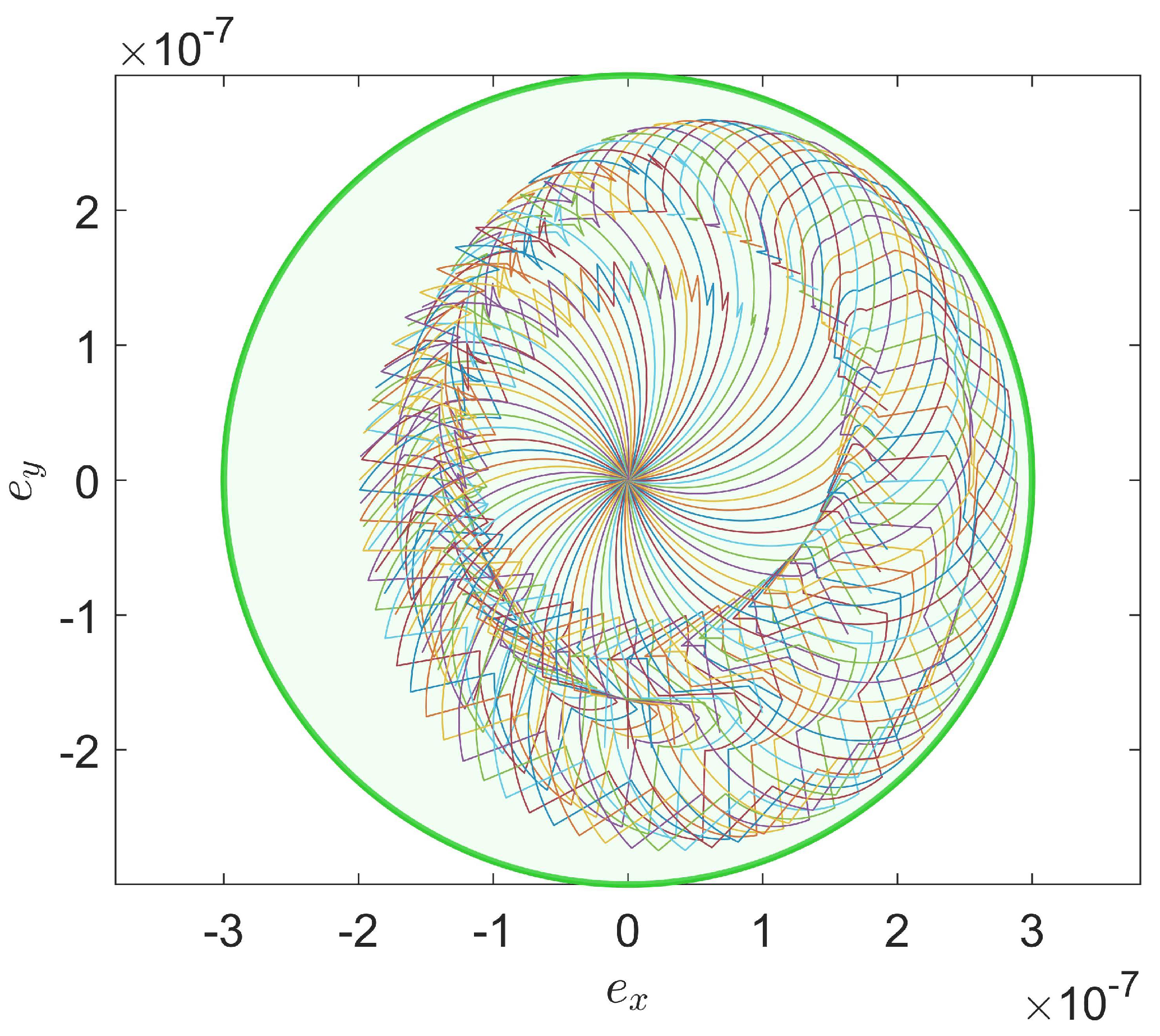
To find a better control effect, we take 6 times eccentricity control for different initial solar radiation direction.

$$\begin{array}{cc}\hfill e_x\left(t\right)& =e_x\left(t_0\right)+\frac{3F_s}{2na}\frac{1}{n_s}[cos{l}_s\left(t\right)-cos{l}_s\left(t_0\right)]cos{i}_s+\sum _{i=1}^6\frac{2}{na}\frac{B}{n_s}[cos{l}_s\left(t_i\right)-cos{l}_s\left(t_{i_0}\right)],\hfill \\ \hfill e_y\left(t\right)& =e_y\left(t_0\right)+\frac{3F_s}{2na}\frac{1}{n_s}[sin{l}_s\left(t\right)-sin{l}_s\left(t_0\right)]+\sum _{i=1}^6\frac{2}{na}\frac{B}{n_s}[sin{l}_s\left(t_i\right)-sin{l}_s\left(t_{i_0}\right)],\hfill \end{array}$$

where

$$\begin{array}{cc}\hfill & B=-5\times {10}^{-11}\mathrm{m}/{\mathrm{s}}^2\hfill \\ \hfill & l_s\left(t_0\right)=0\mathrm{deg},\hfill \\ \hfill & l_s\left(t_{i_0}\right)=60\mathrm{deg}\times i,i=1\cdots 6.\hfill \end{array}$$

Compared Figure 12 with Figure 13, we could know that $e_x,e_y$ are kept staying in the eccentricity limited circle after a Saturn’s year for initial $(e_{x_0},e_{y_0})=(0,0)$ and any given solar radiation direction $l_{s_0}$.

6. Conclusions

In our paper, we analyze the sun-synchronous orbits, repeating ground track orbits, frozen orbits, and stationary orbits around Saturn and corresponding control strategies based on the mean element theory while zonal harmonic coefficients $J_2$ and $J_4$ of Saturnian gravitational field are considered.

For sun-synchronous orbits, we analyze the existence of orbits, find the relation between inclination with eccentricity and semi major axis, and calculate the local time drift caused by solar gravitation and atmospheric drag. After that, we take two inclination-biased control strategies to damp the local time drift. The initial inclination-biased method suits the short-time spacecraft. The periodic inclination biased method has a better effect on long-period missions.

For repeating ground track orbits, we find the meaningful range of repetition parameter Q. Then we find the relation between the inclination and semimajor axis. After that, we calculate the compensation for semimajor axis and maneuver period.

For frozen orbits, we learn that only when $\omega =270$ deg can we be sure of the eccentricity positive for any given inclination and semimajor axis.

For stationary orbits, we first calculate the radius using the conditions of equilibrium point. Then, we analyze the perturbations caused by solar gravitation and solar radiation pressure. Finally, we take corresponding maneuver strategies to control the inclination and eccentricity.