Article

Path Planning Based on NURBS for Hyper-Redundant Manipulator Used in Narrow Space

1
College of Mechanical and Electrical Engineering, Nanjing University of Aeronautics and Astronautics, Nanjing 210016, China
2
Key Laboratory of Measurement and Control of Complex Systems of Engineering, Southeast University, Ministry of Education, Nanjing 210096, China
*
Authors to whom correspondence should be addressed.
Appl. Sci. 2022, 12(3), 1314; https://doi.org/10.3390/app12031314
Submission received: 29 December 2021 / Revised: 21 January 2022 / Accepted: 21 January 2022 / Published: 26 January 2022
(This article belongs to the Section Robotics and Automation)

Abstract

:
Hyper-redundant manipulators with multiple degrees of freedom have special application prospects in narrow spaces, such as detection in small spaces in aerospace, rescue on-site disaster relief, etc. In order to solve the problems of complex obstacle avoidance planning and inverse solution selection of a hyper-redundant robot in a narrow space, a cubic B-spline curve based on collision-free trajectory using environmental edge information is planned. Firstly, a hyper-redundant robot composed of four pairs of double UCR (Universal-Cylindrical-Revolute) parallel mechanisms (2R1T, 2 Rotational DOFs and 1 Translation DOF) in series to realize flexible obstacle avoidance motion in narrow space is designed. The trajectory point envelope of a single UCR and the workspace of a single pair of UCR in Cartesian space based on the motion constraint boundaries of each joint are obtained. Then, the constraint control points according to the edge information of the obstacle are obtained, and the obstacle avoidance trajectory in the constrained space is planned by combining the A* algorithm and cubic B-spline algorithm. Finally, a variety of test scenarios are built to verify the obstacle avoidance planning algorithm. The results show that the proposed algorithm reduces the computational complexity of the obstacle avoidance process and enables the robot to complete flexible obstacle avoidance movement in the complex narrow space.

1. Introduction

With the development of aerospace technology, the demand for on-orbit services such as maintenance of space equipment and fuelling has become more and more urgent. In order to reduce costs and improve the efficiency of astronauts working outside the cabin, many countries or communities have adopted space robots [1] as an important development direction of spacecraft on-orbit services. In European and American, the space robotic arm is mainly carried in the extravehicular environment to assist astronauts to check and repair some space station faults, which reduces the workload of astronauts to a certain extent and avoids the hidden dangers of astronauts’ operations in outer space [2,3,4]. Orbiting service robots for aerospace applications are generally divided into multi-footed crawling robots [5,6,7] and space-operating manipulators [8,9,10,11]. For the routine operation tasks of the space station, such as surface wiping, target detection and grabbing, the space operation robot arm is generally used to complete the task.
With the complexity of its operating environment and the narrowing of its working space, many researchers have set their sights on the research of continuous robots with more degrees of freedom and better bending characteristics [12]. Elastic objects are often used as the body support for continuous robots, and have good bending characteristics and barrier capabilities. It can show different corresponding configurations for different environments and form a smooth curve. It has superior bending characteristics and strong obstacle avoidance ability. It also has strong motion flexibility, which is suitable for the narrowness with obstacles [13,14,15]. Most continuous snake robots achieve passive environmental adaptability through the flexibility of materials or structures [16,17], to achieve the desired position in a complex environment. Nonetheless, this type of robot has low positioning accuracy under load and is hard to achieve accurate control in a small space [18]. The super-redundant hierarchical driven continuous robot can effectively solve the above problems. At present, there is little research on the structure design and motion planning of this type of robot [19,20,21]. In [20], a cable-driven hyper-redundant manipulator with 17 degrees of freedom is presented for narrow and complex environments. Based on the mechanical structure, the MDA + RRT algorithms is proposed for path planning considering the maximum deflection angle of joint. Although this method can be applied to the planning of small spaces, it cannot control the position of the fuselage of each cell of the continuum, and does not consider whether the envelope of the fuselage will collide with the environment.
Obstacle avoidance motion is the motion planning of super-redundant manipulators. For the traditional intelligent algorithm’s obstacle avoidance effect is not strong, scholars [22,23,24,25,26] proposed a path following motion method called follow end trajectory. The characteristic of following the end trajectory is that the links and joints of the super-redundant robotic arm move along the path curve in the restricted area, the entire robotic arm is as close to the path curve as possible in the movement to achieve the smallest possible stroke in space regional goals.
According to analysis, most of the currently designed hyper-redundant manipulators have a series structure, which has low rigidity and poor bearing capacity. In addition, the joint cannot be guaranteed to be on the path curve with low accuracy. At the same time, the solution is complicated and the efficiency is low. Therefore, a hyper-redundant robotic arm trajectory-planning algorithm is provided in this paper. The robotic arm is composed of 8 UCR parallel joints connected in series. The UCR parallel joints have three degrees of freedom that rotate around the X, Y-axis and move around the Z-axis. Parallel mechanism, which consists of a fixed platform, three branch chains, and a moving platform. From the bottom to the top, the branch chain consists of universal, cylindrical, and revolute. The universal joint of the branch chain is connected to the fixed platform, and the rotary pair is connected to the moving platform. With the cooperation of the feeding base, the robot arm moves strictly in accordance with the planned path curve to strictly avoid obstacles.
In summary, the algorithm proposed in this paper has the following advantages:
(1)
It can strictly guarantee that the end of the robot arm is on the cubic B-spline path curve with high accuracy, and the cubic B-spline trajectory G2 is continuous, ensuring smooth movement.
(2)
Solve the pose of the robot arm through the UCR parallel joint drive equation, with high accuracy and fast efficiency.

2. Kinematics Modeling and Workspace Analysis of UCR Parallel Mechanism

Three degrees-of-freedom (DOFs) parallel mechanisms have high accuracy and large loading capacity. This part concentrates on the Kinematics modeling and workspace analysis of UCR parallel mechanism. Firstly, symmetric three-chain with two rotational DOFs and one translation DOF (2R1T) are designed based on constrained screw theory. Secondly, kinematics model of UCR parallel mechanism is constructed. The relative pose of the moving platform and the fixed platform can be adjusted by changing the length of the drive chain. Finally, the workspace analysis is finished based on simulation.

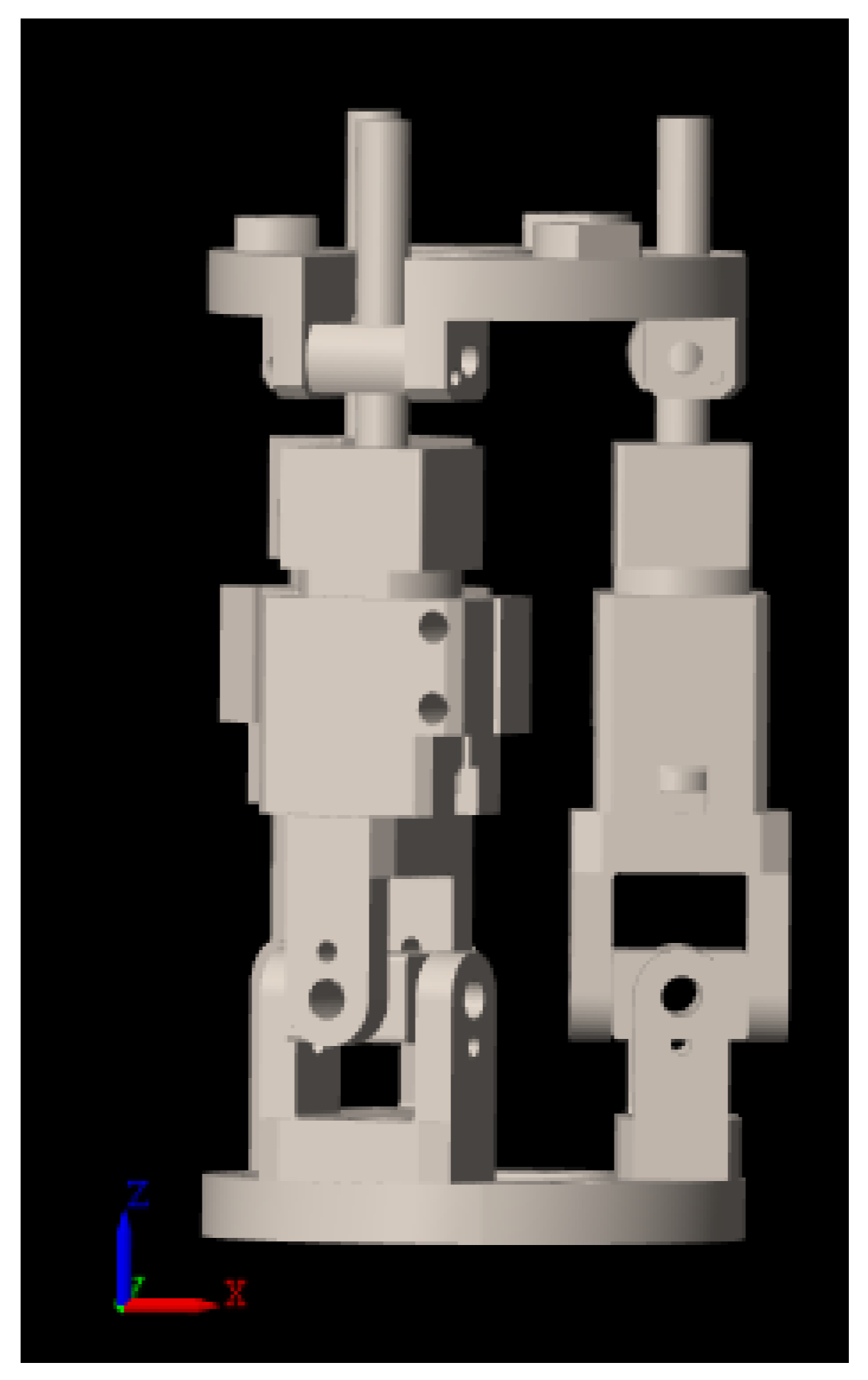
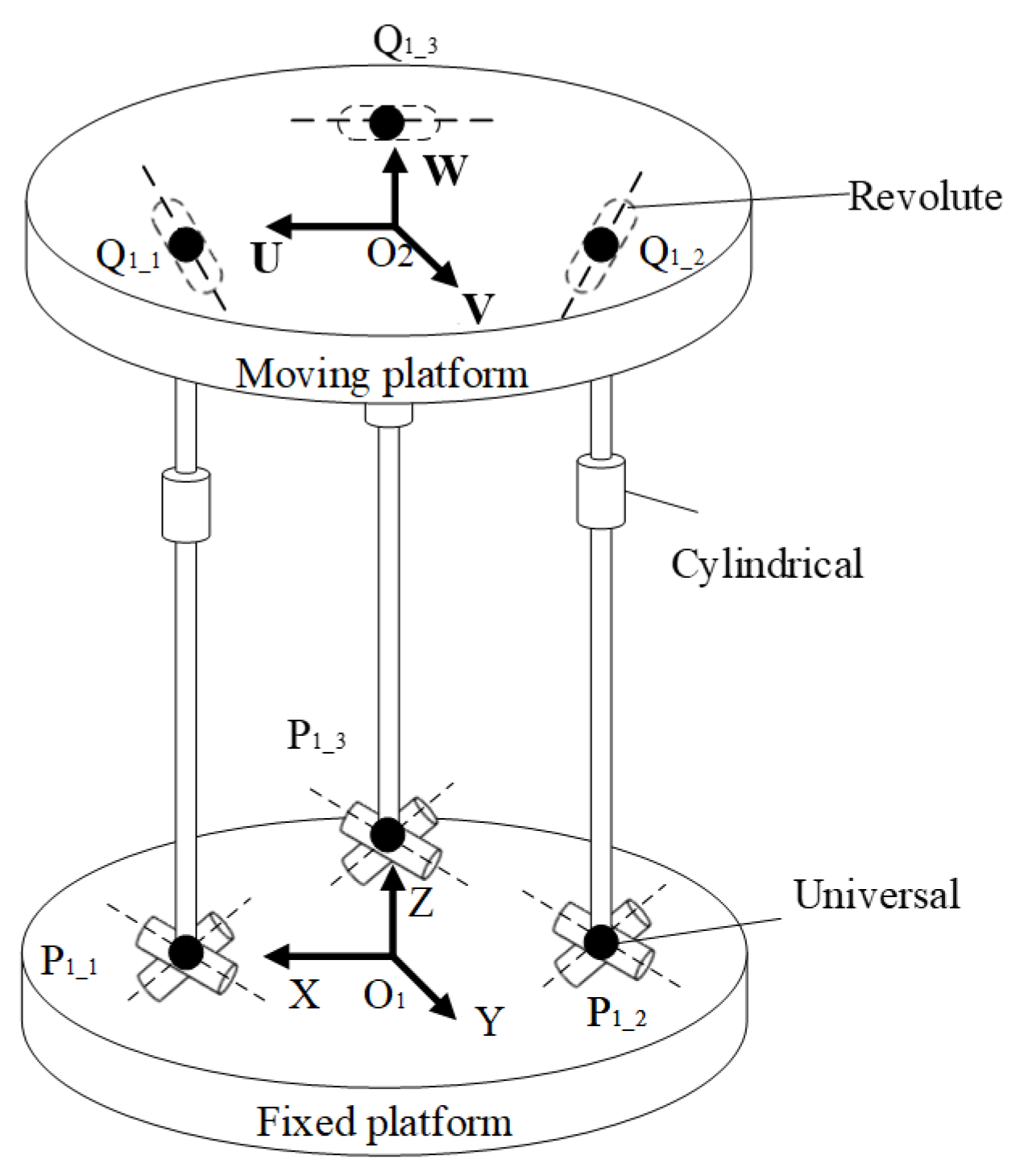
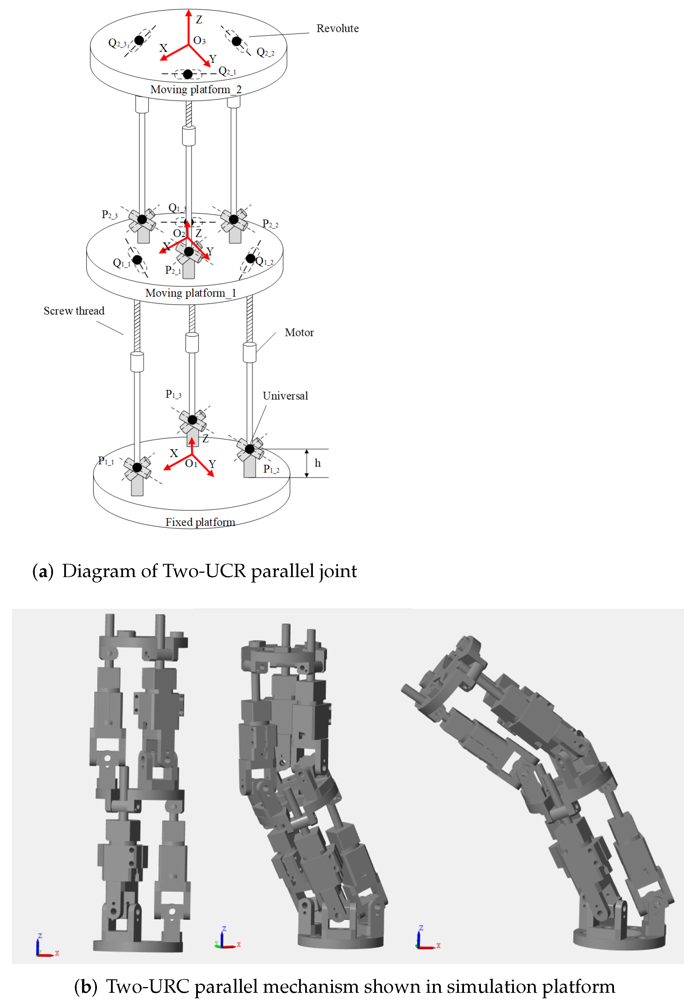
2.1. Introduction of UCR Parallel Mechanism

A three degrees-of-freedom (DOFs) parallel mechanism with two rotational DOFs and one translation DOF (2R1T) is designed based on constrained screw theory. The parallel mechanism consists of a fixed platform, three symmetric chains and a moving platform. The chain is composed of a universal joint, a cylindrical joint and a rotating joint from bottom to top. As shown in Figure 1, the cylindrical joint is a motor-driven pair, which is expanded and contracted through the cylindrical joint to adjust the position of the moving platform. In the initial state, the attitude of the flexible joint moving platform is the same as that of the fixed platform.

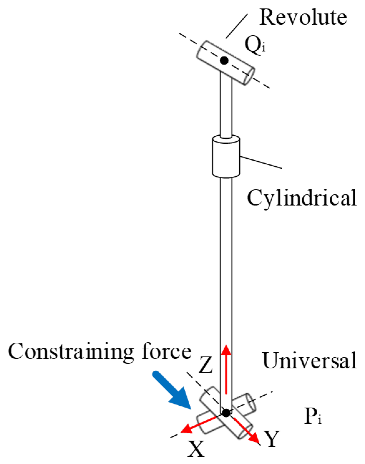
2.2. Kinematics Modeling of UCR Parallel Mechanism

(1)
The driven model of UCR parallel mechanism
As shown in Figure 1, O 1 and O 2 are the center of the fixed platform and the moving platform, respectively. The connection points of the three chains to the fixed platform and the moving platform are P 1 _ i , Q 1 _ i ( i = 1 , 2 , 3 ) . The radius of the fixed platform and moving platform is r. A fixed coordinate system O X Y Z is established on the fixed platform. The two orthogonal axes of the universal joint are used as the X and Y-axes, where the X-axis points from O 1 to P 1 _ 1 , and the Z axis is the fixed platform normal. A moving coordinate system O 2 U V W is established on the moving platform, where the U axis is from O 2 to Q 1 _ 1 , and the W axis is the normal of the moving platform.
The transformation matrix of moving coordinate system O 2 U V W relative to fixed coordinate system O 1 X Y Z is
T = n x o x a x X c n y o y a y Y c n z o z a z Z c 0 0 0 1
The coordinates of P 1 _ 1 , P 1 _ 2 , and P 1 _ 3 in the coordinate system O 1 X Y Z are:
P 1 _ 1 = r 0 0 P 1 _ 2 = r 2 3 r 2 0 P 1 _ 3 = r 2 3 r 2 0
The coordinates of Q 1 _ 1 , Q 1 _ 2 , and Q 1 _ 3 in the coordinate system O 2 U V W are:
Q 1 _ 1 = r 0 0 Q 1 _ 2 = r 2 3 r 2 0 Q 1 _ 3 = r 2 3 r 2 0
Because of Q i 1 = T Q 1 _ i 1 ( i = 1 , 2 , 3 ) , so
Q 1 = Q 1 x Q 1 y Q 1 z = r n x + X c r n y + Y c r n z + Z c
Q 2 = Q 2 x Q 2 y Q 2 z = r 2 n x + 3 r 2 o x + X c r 2 n y + 3 r 2 o y + Y c r 2 n z + 3 r 2 o z + Z c
Q 3 = Q 3 x Q 3 y Q 3 z = r 2 n x 3 r 2 O x + X c r 2 n y 3 r 2 O y + Y c r 2 n z 3 r 2 O z + Z c
The driving functions is obtained as follows:
l 1 _ i 2 = Q 1 _ i P 1 _ i 2 = R Q 1 _ i + c P 1 _ i T R Q 1 _ i + c P 1 _ i ( i = 1 , 2 , 3 )
where l 1 _ i represents the length of chain.
(2)
The constraint model of UCR parallel mechanism
The chains of the UCR parallel mechanism are symmetric. Take one of the chains and analyze its motion spiral and constraint spiral. The chain is shown in Figure 2.
According to the screw theory, the screw system of the chain is:
$ 1 = ( 1 , 0 , 0 ; 0 , 0 , 0 ) $ 2 = ( 0 , 1 , 0 ; 0 , 0 , 0 ) $ 3 = ( 0 , 0 , 1 ; 0 , 0 , 0 ) $ 4 = ( 0 , 0 , 0 ; 0 , 0 , 1 ) $ 5 = ( 0 , 1 , 0 ; l i , 0 , 0 )
Constrained screw is:
$ r = ( 0 , 1 , 0 ; 0 , 0 , 0 )
Three constraint equations are obtained as follows:
n y = o x X c = r ( n x o y ) 2 Y c = r n y
(3)
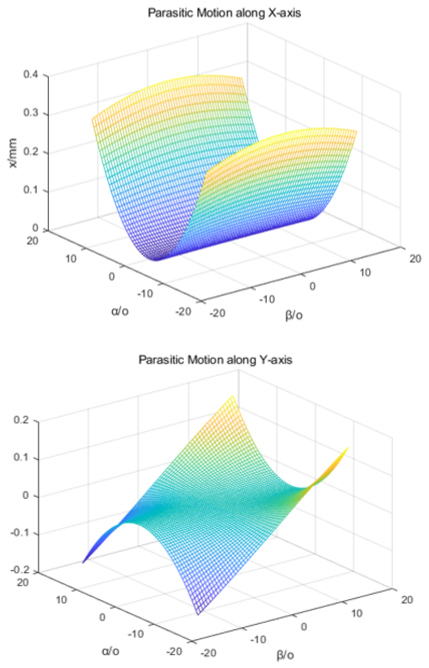
The parasitic motion of UCR parallel mechanism
Attitude description based on Z X Z Euler Angle:
R = C α 2 + S α 2 C β C α S α ( 1 C β ) S α S β S α C α ( 1 C β ) S α 2 + C α 2 C β C α S β S α S β S β C α C β
The rotation matrix is equivalent to rotate the β degrees around the axis that is α degrees from the X-axis. The parasitic motion is defined as: when the parallel mechanism performs a rotating motion, the moving motion accompanying the platform is called parasitic motion. The parasitic motion of the UCR parallel joint is independent of Z-axis, and the expression is as follows:
X M = X c X o = r cos ( 2 α ) ( 1 cos β ) 2
Y M = Y c Y o = r sin ( 2 α ) ( 1 cos β ) 2
Let r = 20 m, α [ 15 , + 15 ] , β [ 15 , + 15 ] , the parasitic motion based on constraint equations is shown in Figure 3.

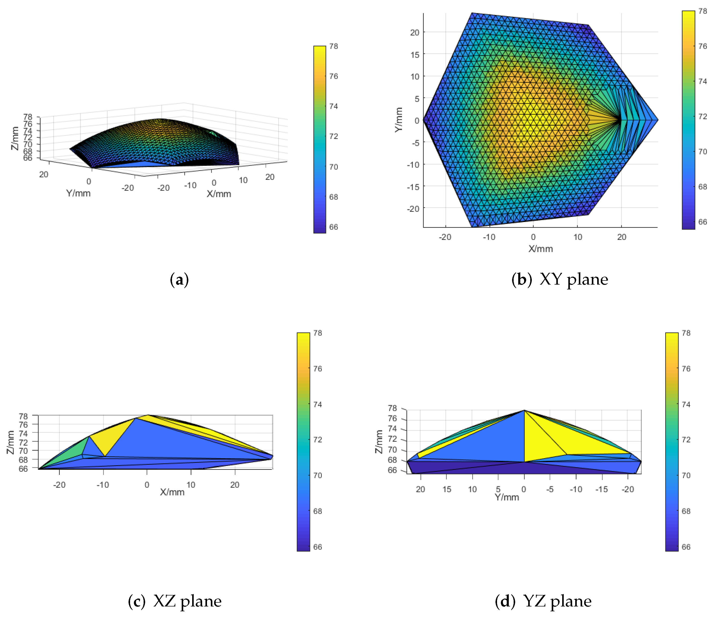
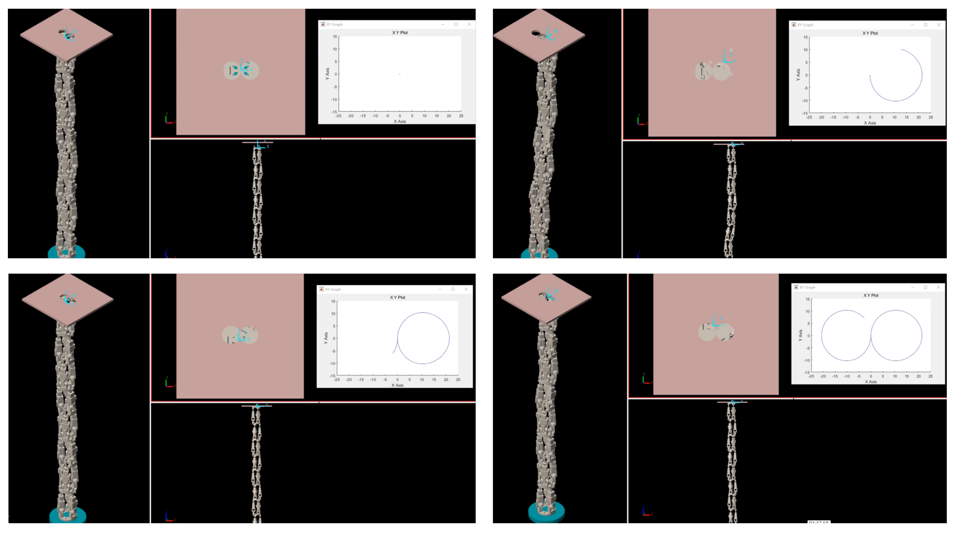
2.3. Workspace Analysis Based on Simulation

In this section, the 3D CAD model of the UCR parallel mechanism is imported into simulation, and the simulation platform is used to analyze its working space. The simulation platform is shown in Figure 4.
Through the position sensor module, the position information of UCR parallel mechanism is obtained, and simulation is used to form the track point envelope. As shown in Figure 5a–d. The envelope is cloak-shaped and symmetrically divided into three equal parts along the central axis.

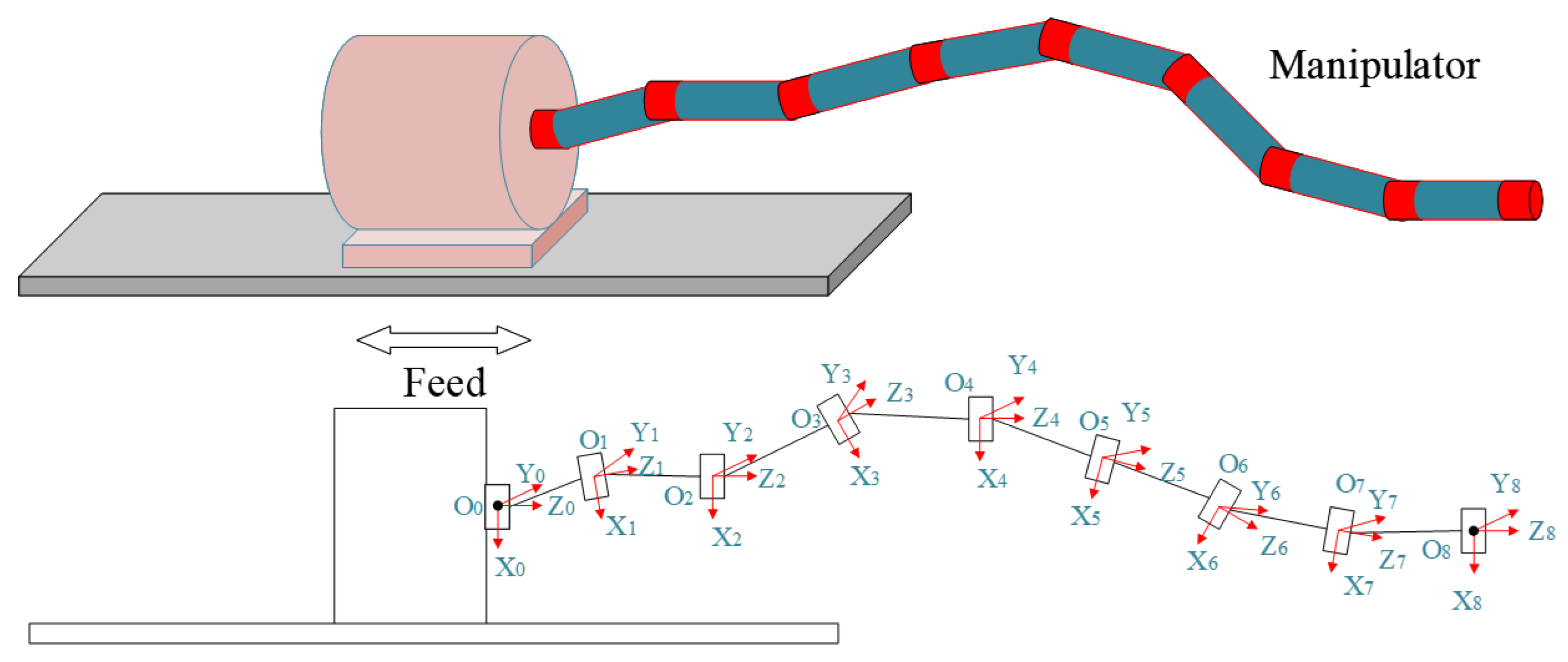
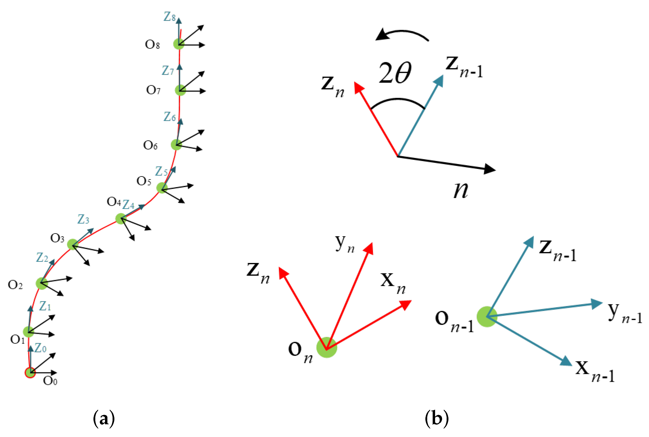
3. Kinematics Modeling of the Manipulator

Three degrees-of-freedom (DOFs) parallel mechanisms have high accuracy, large loading capacity. This work concentrates on the Kinematics modeling of the manipulator.

3.1. Kinematics Modeling of the Manipulator

The manipulator consists of eight UCR parallel mechanisms (also regarded as four identical double-UCR parallel mechanism units). Each mechanism rotates 60 alternately. Four double-UCR mechanism units work together to finish the task of path planning in free space.
As shown in Figure 6, the Z-axis of the coordinate is along the normal direction of the platform. The rotation matrix of UCR parallel mechanism between fixed platform and moving platform is expressed as follows:
n n 1 T = T r a n s ( X c , Y c , Z c ) R Y ( β ) R X ( α ) = cos ( β ) sin ( α ) sin ( β ) sin ( β ) cos ( α ) X c 0 cos ( α ) sin ( α ) Y c sin ( β ) cos ( β ) sin ( α ) cos ( α ) cos ( β ) Z c 0 0 0 1
where α , β ( 90 , 90 ) , α , β and X c , Y c , Z c are mutually coupled variables. The transformation matrix of i-th platform with respect of the base can be obtained by following equation:
i 0 T = 1 0 T 2 1 T 3 2 T i 1 i 2 T i i 1 T ( i = 1 , 2 , , 8 )

3.2. Kinematics Modeling of Double-UCR Parallel Mechanisms

The relative coordinate system between the first moving platform and the second platform is shown in Figure 7a and the structure of the two-UCR parallel mechanisms is shown in Figure 7b.
The drive motor is distributed longitudinally, and the linear movement of the threaded pair can pass through the moving platform. By the motor drive, the attitudes of the moving platform 1 and the moving platform 2 are adjusted, thereby determining the relative movement of the end coordinate system O i -UVW relative to the fixed platform coordinate system O 1 -XYZ. Among them, the distance between the joint center of rotation of the gimbal and the fixed platform is h = 13.5 mm, and the stroke of the rotation radius r = 15 mm is 5–20 mm.

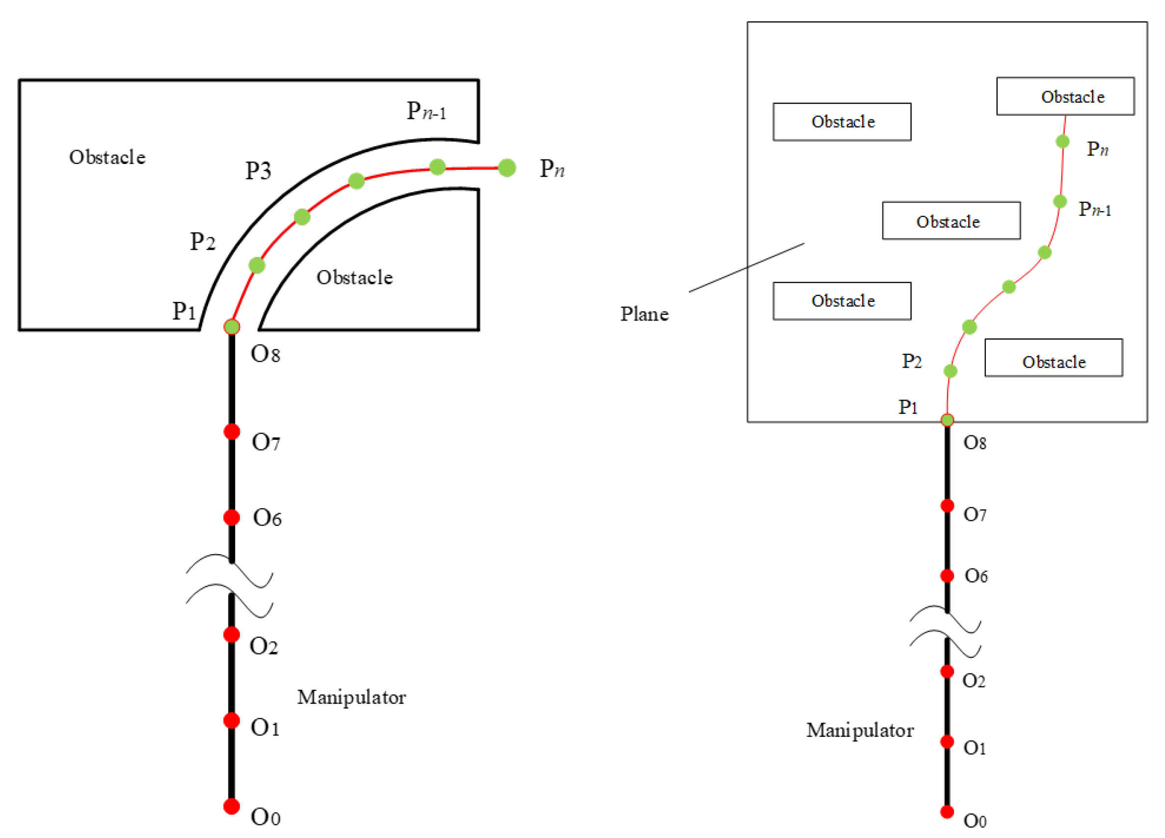
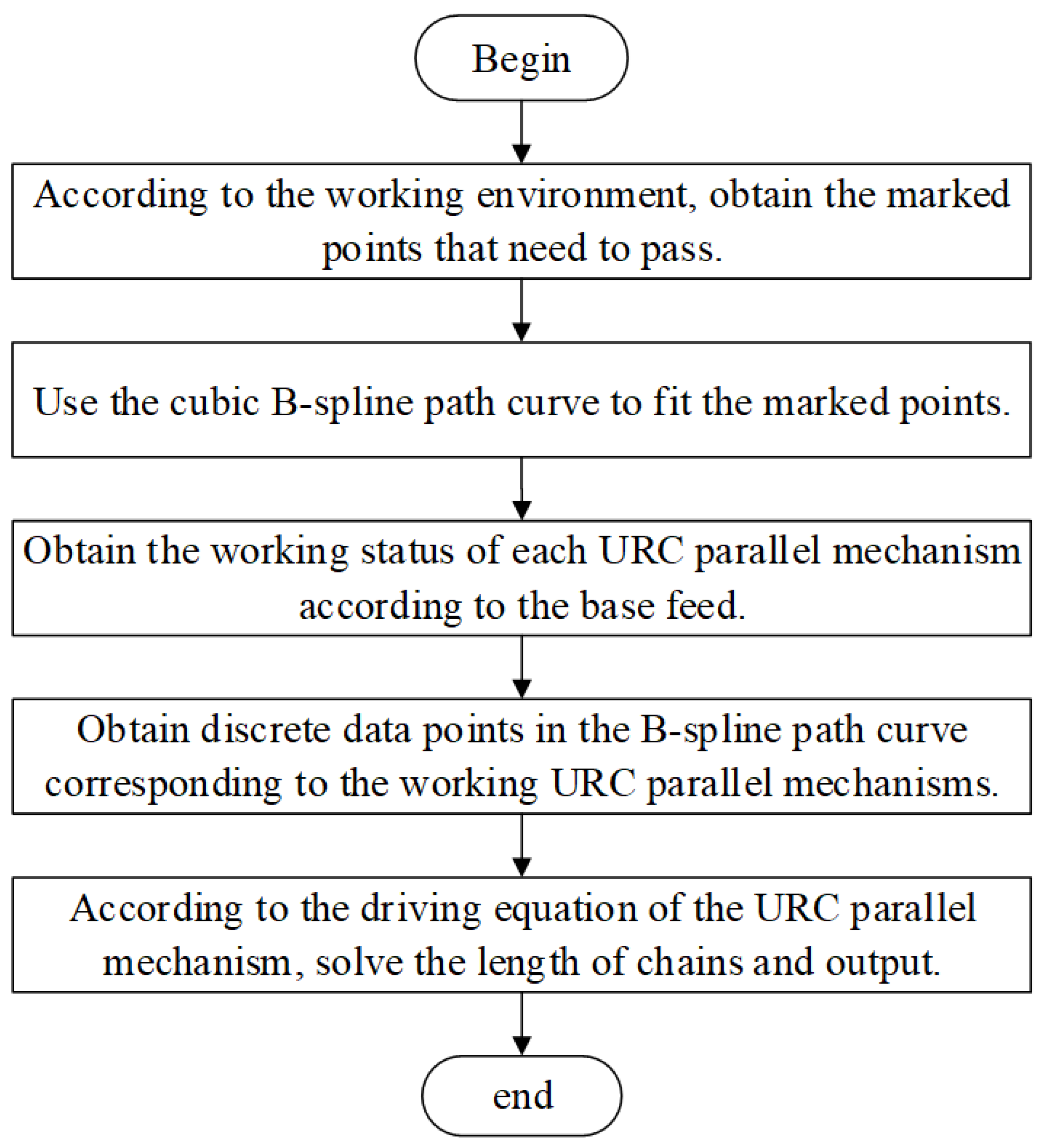
4. The Tip-Following B-Spline Path Planning

The realization of tip-following B-spline trajectory in a continuous path includes five parts: (1) Obtaining the marked points P 1 P n that need to pass according to the working environment. (2) Using the cubic B-spline path curve to fit the marked points, then generate a cubic B-spline path curve. (3) Obtain the working status of each UCR parallel joint according to the base feed. (4) In the B-spline path curve, obtain discrete data points corresponding to the working UCR parallel mechanism. (5) According to the driving equation of the UCR parallel joints, solve the rod length of each joint and output it. The algorithm flow chart is shown in Figure 8.
When environment parameters are obtained, path planning can be automatically generated by A * algorithm, ant colony algorithm, etc. Alternatively, through manual marking, we can obtain the marking points P 1 P n , which the working space needs to pass. The working conditions and marked points of the hyper-redundant robotic arm are shown in Figure 9.
For the four-UCR parallel mechanisms, the maximum rotation angle along the X-axis is 99 . 36 and the radius of curvature is 167 mm. The maximum rotation angle along the Y-axis is 90 . 57 and the radius of curvature is 184 mm, as shown in Figure 10.
B-spline curve is widely used in tool path fitting due to its versatility and easy realization. B-splines can be defined by control points and node vectors. Using them to represent tool paths can simplify code and reduce data storage. In addition, the B-spline itself has high continuity, and the cubic B-spline curve is G2 continuous, and the fitted trajectory has better smoothness, and the original data points are passed to strictly guarantee the fitting accuracy.
The cubic B-spline curve is defined as: ( u ) = i = 0 n N i , k ( u ) P i , u [ 0 , 1 ] . Where P i ( i = 0 , 1 , , n ) is the control points. N i , k ( t ) ( i = 0 , 1 , , n ) is the basis functions. k = 3 . The node vector U = { 0 , 0 k + 1 , u k + 1 , , u n , 1 , , 1 k + 1 } . We use nonperiodic node vector, which is obtained by using a binary search on the node vector when determining the node interval to which u belongs. The trajectory of the marked points P 1 P n after fitting by the cubic B-spline curve is shown in Figure 11.
According to the feed amount F D of the base, the motion state of each UCR parallel mechanism is sequentially judged. Assume that the end of the robot arm is the starting point of the cubic B-spline spline trajectory, and the initial length of the UCR parallel joint I n D i s . Then, first calculate the number of UCR parallel joints in the working state: N u m = c e i l ( F D / I n D i s ) , and the function c e i l ( ) means rounding up. Because the robotic arm starts to move from the end, the UCR parallel joint index in the working state is: 9 N u m 8 (the index of the UCR joint is 1 to 8, respectively).
The tangential direction of a B-spline curve c ( t ) at the discrete point is the Z axis of the point. Assuming that the parameters corresponding to two adjacent discrete points are t ( n 1 ) and t n , the corresponding discrete points are: c ( t ( n 1 ) ) and c ( t n ) . Then, Z ( n 1 ) and Z n are unit vectors of c ( t ( n 1 ) ) and c ( t n ) , respectively. The 3D vector rotation represented by quaternion is shown in Figure 11a,b.
In 3D space, the unit vector n rotate 2 θ can use the quaternion q = [ cos θ , n sin θ ] = q 0 + q 1 i + q 2 j + q 3 k to describe.
Where n = z n 1 × z n z n 1 × z n , 2 θ = arccos ( z n 1 z n ) .
The rotation matrix n n 1 R represented by rotation quaternion q = ( q 0 , q 1 , q 2 , q 3 ) T is:
n n 1 R = q 0 2 + q 1 2 q 2 2 q 3 2 2 ( q 1 q 2 q 0 q 3 ) 2 ( q 1 q 3 q 0 q 2 ) 2 ( q 1 q 2 q 0 q 3 ) q 0 2 q 1 2 + q 2 2 q 3 2 2 ( q 2 q 3 q 0 q 1 ) 2 ( q 1 q 3 q 0 q 2 ) 2 ( q 2 q 3 q 0 q 1 ) q 0 2 + q 1 2 q 2 2 + q 3 2
Assuming coordinate system O n 1 x n 1 y n 1 z n 1 is known. According to the relative pose description, it can be known that the coordinates of O n projected at the coordinate system are:
n n 1 Z = n n 1 X c , n n 1 Y c , n n 1 Z c T
According to the transformation relationship between the relative coordinate systems, it can be known that the transformation matrix between two adjacent discrete points is:
n n 1 T = n n 1 R n n 1 Z 0 1
The base coordinate system O 0 x 0 y 0 z 0 of manipulator is given in advance, and described as:
O 0 x 0 y 0 z 0 = 1 0 0 0 1 0 0 0 1 , O 0 = 0 0 0
Find the first discrete point on the B-spline curve by dichotomy method in t [ 0 , 1 ] . Suppose the corresponding parameter is t 1 . Then, compute the coordinate system O 1 x 1 y 1 z 1 and record. Find the second discrete point on the B-spline curve by dichotomy method in t [ t 1 , 1 ] . Similarly, the discrete points corresponding to the all UCR parallel mechanisms can be acquired. The steps for computing each UCR parallel mechanism are:
(1)
Compute the rotation matrix between two adjacent discrete points.
(2)
Determine the parity of the index of the UCR parallel mechanism. If the index is an odd number, use the driving equation CalDrivingLength_1() to compute the length of chains; if the index is even, use the driving equation CalDrivingLength_2() to compute the length of three chains.
Pseudo-code of CalDrivingLength_1() and CalDrivingLength_2() is introduced below.
Pseudo-code of CalDrivingLength_1():
ine FUNCTION: CalDrivingLength_1 ( T 1 , r )
INPUT: T 1 / / Transformation matrix of moving platform
r / / The distance between P ( 1 _ 1 ) and O 1
OUTPUT: l ( 1 _ 1 ) , l ( 1 _ 2 ) , l ( 1 _ 3 ) / / The length of the three chains
BEGIN
   1. n x o x a x X c n y o y a y Y c n z o z a z Z c 0 0 0 1 call Translate ( T 1 )
   2. P 1 _ 1 r 0 0 ; P 1 _ 2 r 2 3 r 2 0 ; P 1 _ 3 r 2 3 r 2 0
   3. Q 1 _ 1 r n x + X c r n y + Y c r n z + Z c ; Q 1 _ 2 r 2 n x + 3 r 2 o x + X c r 2 n y + 3 r 2 o y + Y c r 2 n z + 3 r 2 o z + Z c ; Q 1 _ 3 r 2 n x 3 r 2 o x + X c r 2 n y 3 r 2 o y + Y c r 2 n z 3 r 2 o z + Z c
   4. l 1 _ 1 ( Q 1 _ 1 P 1 _ 1 ) T ( Q 1 _ 1 P 1 _ 1 ) ; l 1 _ 2 ( Q 1 _ 2 P 1 _ 2 ) T ( Q 1 _ 2 P 1 _ 2 ) ; l 1 _ 3 ( Q 1 _ 3 P 1 _ 3 ) T ( Q 1 _ 3 P 1 _ 3 ) ;
   5. Output l 1 _ 1 , l 1 _ 2 , l 1 _ 3
END
ine
Pseudo-code of CalDrivingLength_2() :
ine FUNCTION: CalDrivingLength_2 ( T 2 )
INPUT: T 2 / / Transformation matrix of two moving platforms
OUTPUT: l ( 2 _ 1 ) , l ( 2 _ 2 ) , l ( 2 _ 3 ) / / The length of the three chains
BEGIN
   1. n x o x a x X c n y o y a y Y c n z o z a z Z c 0 0 0 1 call Translate ( T 2 )
   2. P 2 _ 1 r 2 3 r 2 0 r 0 0 ; P 2 _ 2 r 0 0 ; P 2 _ 3 r 2 3 r 2 0
   3. Q 2 _ 1 r 2 n x + 3 r 2 o x + X c r 2 n y + 3 r 2 o y + Y c r 2 n z + 3 r 2 o z + Z c ; Q 1 _ 2 r n x + X c r n y + Y c r n z + Z c ; Q 1 _ 3 r 2 n x 3 r 2 o x + X c r 2 n y 3 r 2 o y + Y c r 2 n z 3 r 2 o z + Z c
   4. l 2 _ 1 ( Q 2 _ 1 P 2 _ 1 ) T ( Q 2 _ 1 P 2 _ 1 ) ; l 2 _ 2 ( Q 2 _ 2 P 2 _ 2 ) T ( Q 2 _ 2 P 2 _ 2 ) ; l 2 _ 3 ( Q 2 _ 3 P 2 _ 3 ) T ( Q 2 _ 3 P 2 _ 3 ) ;
   5. Output l 2 _ 1 , l 2 _ 2 , l 2 _ 3
END
ine

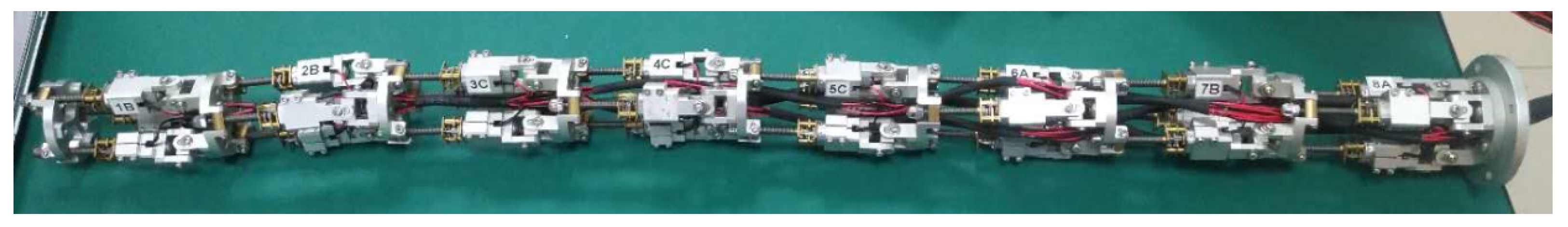
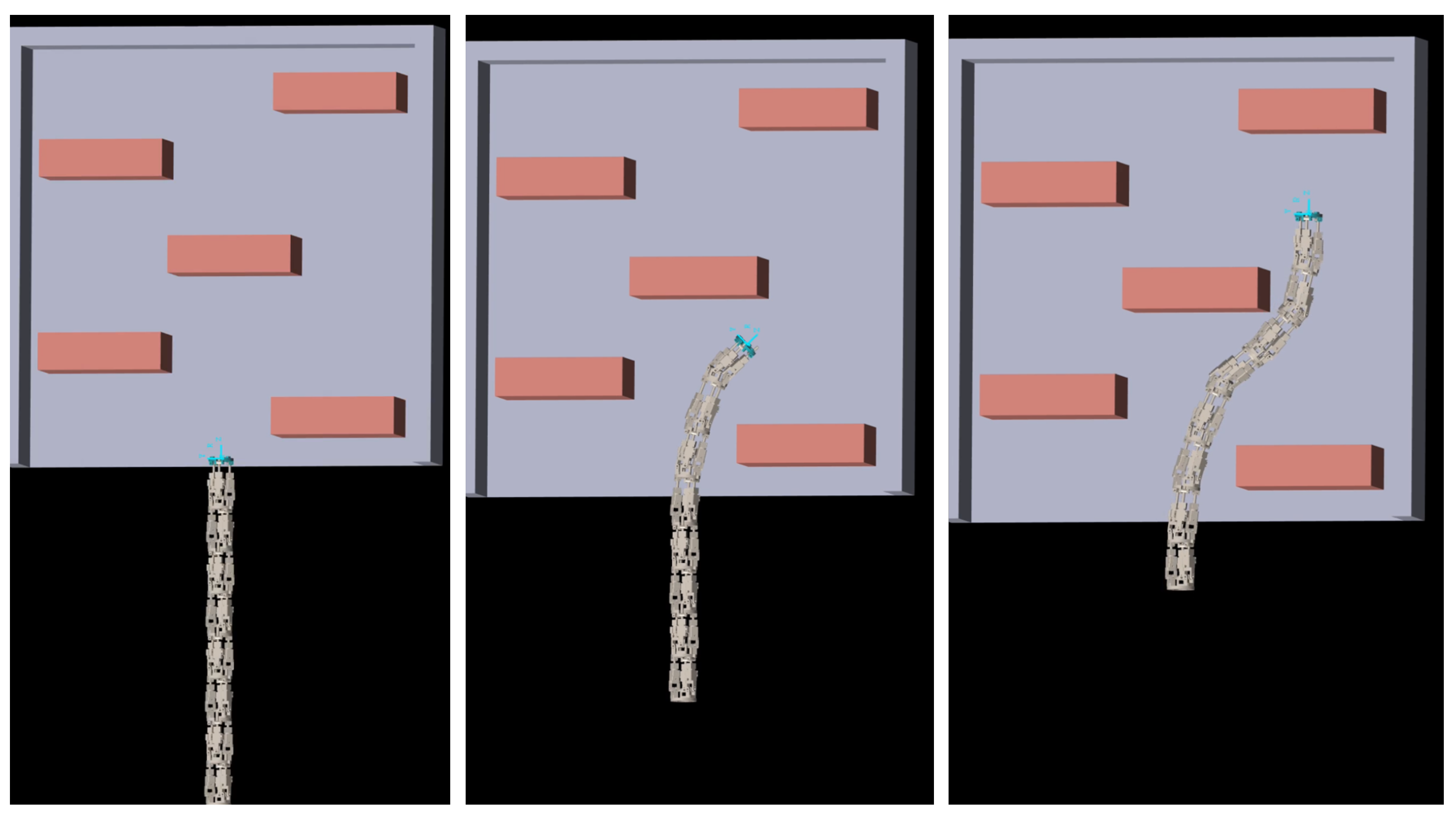
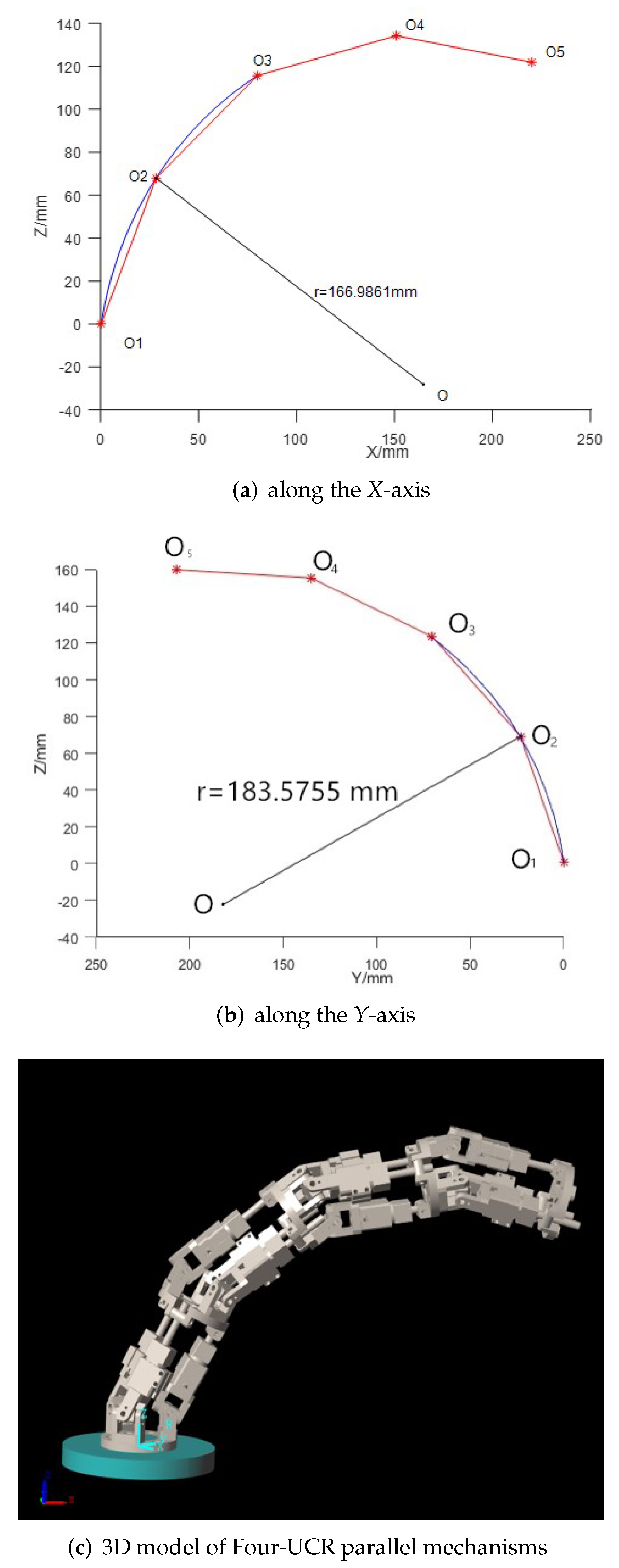
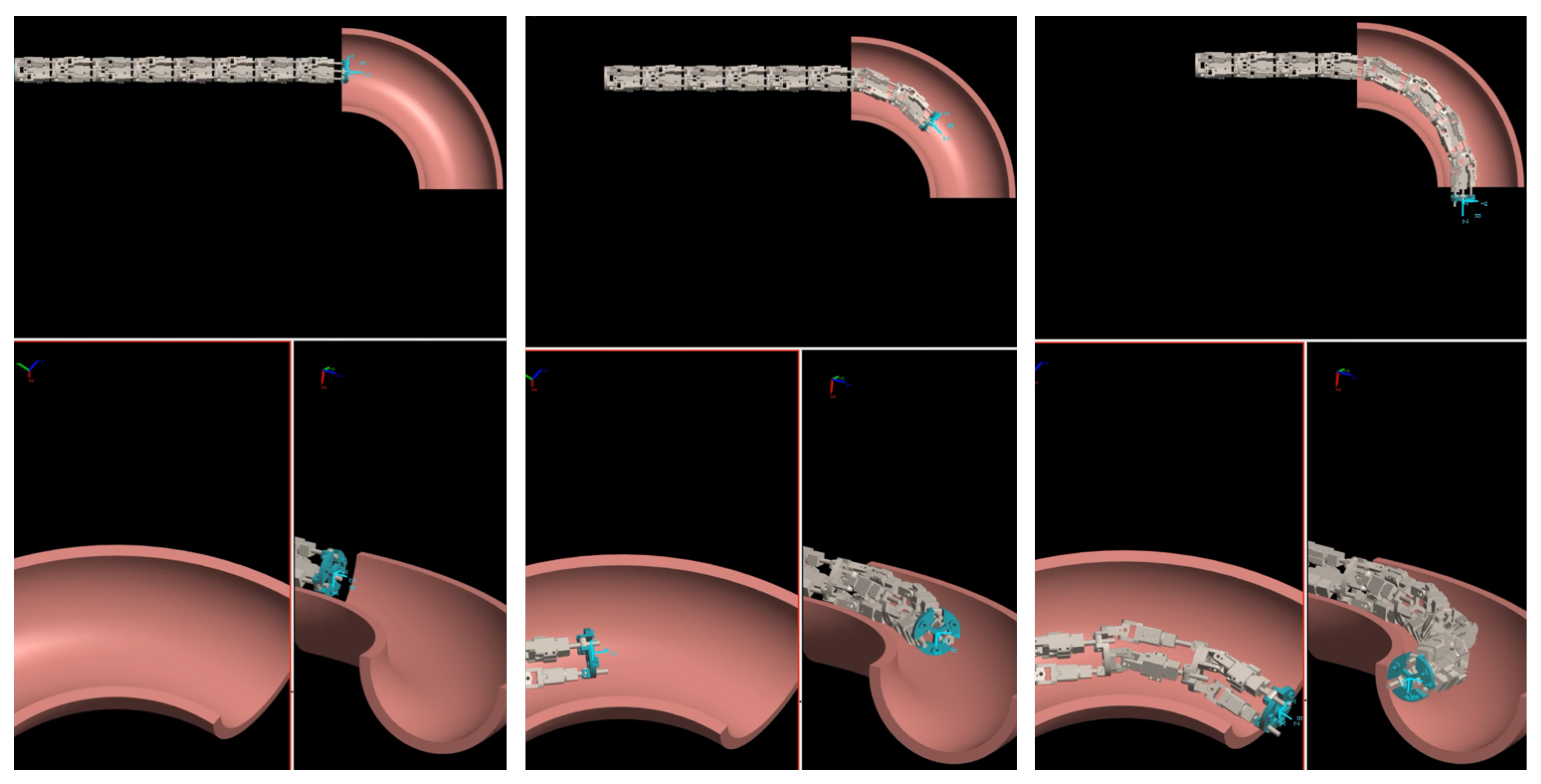
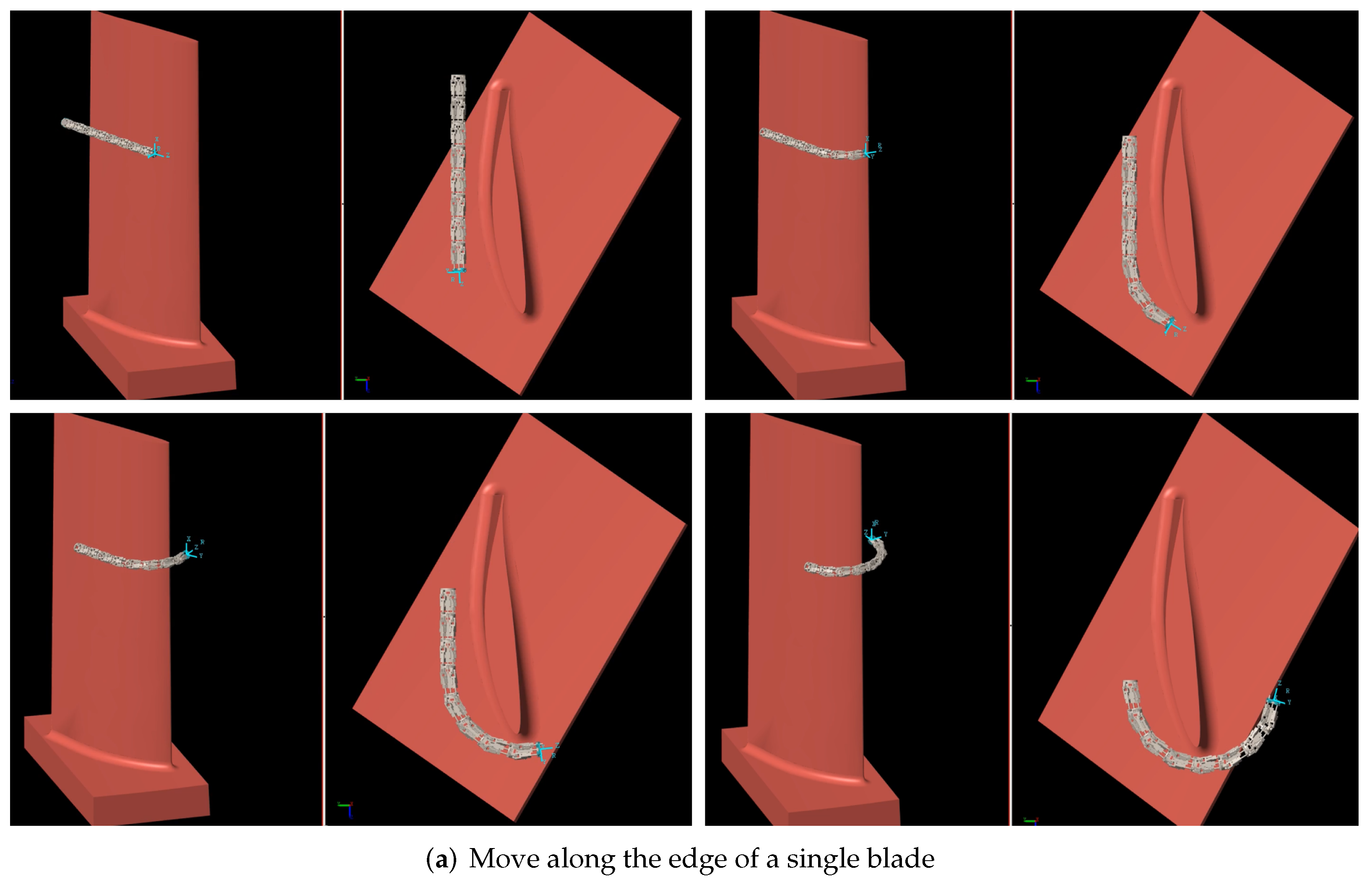
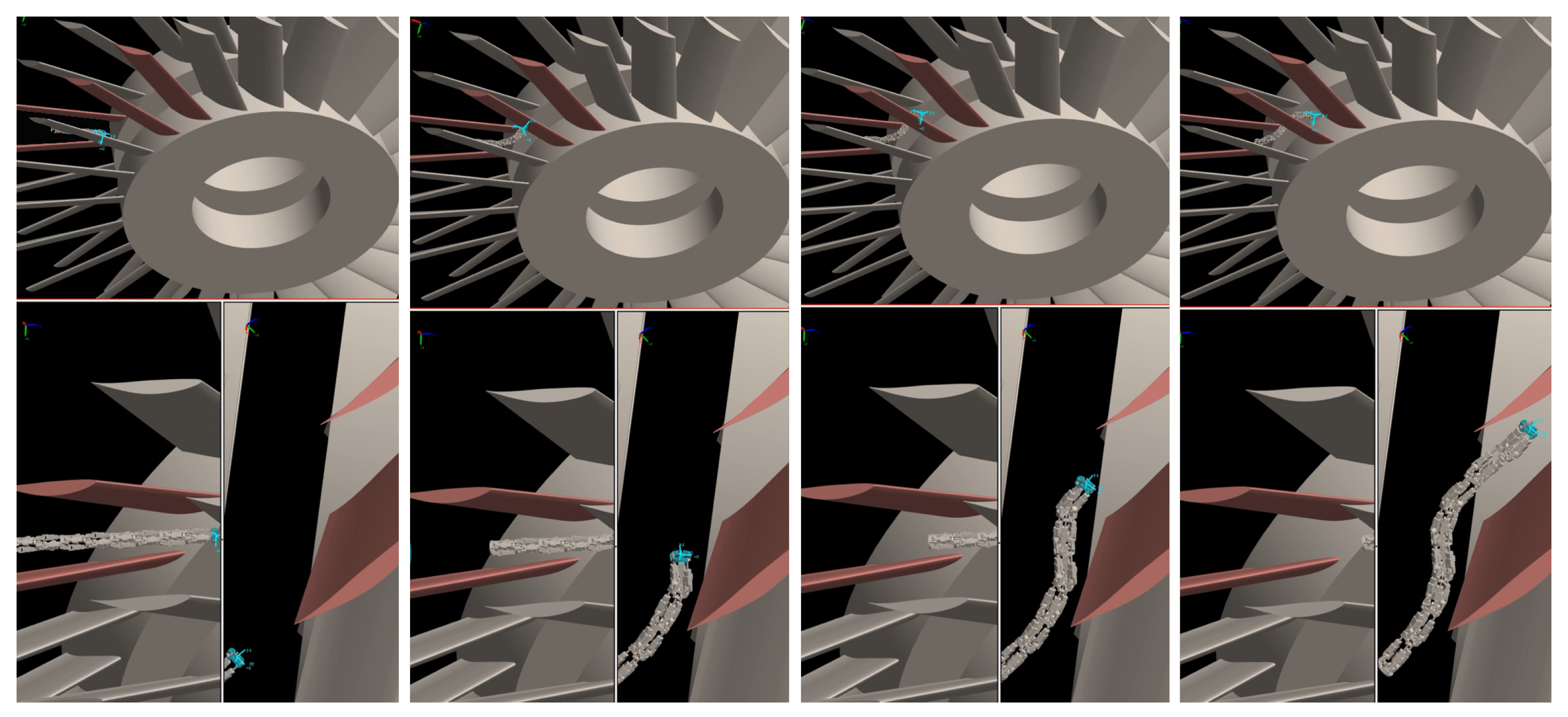
5. Simulations and Experiments

As shown in Figure 12, the arm has eight joints, with an initial length of 544 mm and a diameter of 40 mm.
The schematic diagram of the simulation platform is shown in Figure 13, and the simulation platform consists of four parts: the simulation configuration environment, URC parallel mechanism, signal sensor and position sensor, and the position sensor is incorporated in moving platform.
The robot arm can move smoothly on the plane, as shown in Figure 14. The “8” shape drawn by the robot arm on the plane shows that the robot arm can perform a series of motions stably.
As shown in Figure 15, the hyper-redundant robot can successfully automatically identify roadblocks in space and complete the obstacle avoidance movement through the algorithm.
Because of the small size of the hyper-redundant robot designed in this paper, it can complete the task in the narrow space. As shown in Figure 16, the robot can automatically identify the path to complete the movement and complete the maintenance and other tasks in the pipeline.
The hyper-redundant robot designed in this paper can complete some complex, dangerous and boring tasks. In particular, the generator blades of the nuclear power plant need to be overhauled every year, and the nuclear power plant can not avoid radiation, which is generally harmful to the human body, so it is necessary to use robots to replace human beings to complete dangerous work. As shown in Figure 17, the hyper-redundant robot designed in this paper can travel freely between narrow blades to complete the maintenance and maintenance of engine blades.

6. Conclusions

In this paper, a hyper-redundant robot composed of four pairs of double UCR (Universal-Cylindrical-Revolute) parallel mechanisms (2R1T, 2 Rotational DOFs and 1 Translation DOF) in series to realize flexible obstacle avoidance motion in narrow spaces is designed. Then, a method combining cubic B-spline algorithm with A * Algorithm is proposed to plan the trajectory of obstacle avoidance for hyper-redundant robot in constrained space. The experimental results show that the robot can move smoothly in a plane or inclined plane, it can also travel freely in the narrow space between engine blades. The proposed algorithm reduces the computational complexity of the obstacle avoidance process of hyper-redundant robots and, at the same time, the robot can avoid obstacles flexibly in the complex narrow space.
By setting various simulation test environments, it can be seen that the algorithm proposed in this paper can make the hyper-redundant manipulator pass through many restricted spaces, laying a theoretical foundation and experimental method for the detection of narrow spaces. However, the redundant arm designed in this paper still has certain limitations. For example, the existing mechanical arm has a small load, and a larger motor can be used to improve the load capacity in the future.

Author Contributions

Methodology, J.D., B.W.; validation and data curation, B.W., J.D.; writing—original draft preparation, J.D., B.W., K.C.; writing—review and editing, J.D., K.C., B.W.; visualization, J.D.; supervision, Z.D.; project administration, Z.D.; funding acquisition, Z.D. All authors have read and agreed to the published version of the manuscript.

Funding

This research was funded by National Key Research and Development Plan under grant number 2018YFB1305601. and Open Project Program of the Key Laboratory of Measurement and Control of Complex Systems of Engineering, Ministry of Education, Southeast University under grant number MCCSE2021A04. and the Fundamental Research Funds for the Central Universities under grant number MCCSE2021A04.

Conflicts of Interest

The authors declare no conflict of interest.

References

  1. Freitas, R.A., Jr.; Healy, T.J.; Long, J.E. Advanced automation for space missions. J. Astronaut. Sci. 1982, 30, 221. [Google Scholar]
  2. Heemskerk, C.J.M.; Visser, M.; Vrancken, D. Extending ERA’s capabilities to capture and transport large payloads. In Proceedings of the 9th ESA Workshop on Advanced Space Technologies for Robotics and Automation, Noordwijk, The Netherlands, 28–30 November 2006; pp. 1–8. [Google Scholar]
  3. Cruijssen, H.J.; Ellenbroek, M.; Henderson, M.; Petersen, H.; Verzijden, P.; Visser, M. The European Robotic Arm: A HighPerformance Mechanism Finally on Its Way to Space; NASA: Washington, DC, USA, 2014.
  4. Boumans, R.; Heemskerk, C. The European robotic arm for the international space station. Robot. Auton. Syst. 1998, 23, 17–27. [Google Scholar]
  5. Kingsley, D.A.; Quinn, R.D.; Ritzmann, R.E. A cockroach inspired robot with artificial muscles. In Proceedings of the 2006 IEEE/RSJ International Conference on on Intelligent Robots and Systems (IROS), Beijing, China, 9–15 October 2006; pp. 1837–1842. [Google Scholar]
  6. Luk, B.L.; Cooke, D.S.; Galt, S.; Collie, A.A. Intelligent legged climbing service robot for remote maintenance applications in hazardous environments. Robot. Auton. Syst. 2005, 53, 142–152. [Google Scholar]
  7. Saunders, A.; Goldman, D.I.; Full, R.J.; Buehler, M. The rise climbing robot: Body and leg design. In Proceedings of the Unmanned Systems Technology VIII, International Society for Optics and Photonics, Kissimmee, FL, USA, 17–20 April 2006; Volume 6230, p. 623017. [Google Scholar]
  8. Lovchik, C.S.; Diftler, M.A. The robonaut hand: A dexterous robot hand for space. In Proceedings of the 1999 IEEE International Conference on Robotics and Automation, Detroit, MN, USA, 10–15 May 1999; Volume 2, pp. 907–912. [Google Scholar]
  9. Yu, D.Y.; Sun, J.; Ma, X.R. Suggestion on development of Chinese space manipulator technology. Spacecr. Eng. 2007, 16, 1–8. [Google Scholar]
  10. Laryssa, P.; Lindsay, E.; Layi, O.; Marius, O.; Nara, K.; Aris, L.; Ed, T. International space station robotics: A comparative study of ERA, JEMRMS and MSS. In Proceedings of the 7th ESA Workshop on Advanced Space Technologies for Robotics and Automation, Noordwijk, The Netherlands, 19–21 November 2002; pp. 1–8. [Google Scholar]
  11. Zhang, K.F.; Zhou, H.; Wen, Q.P.; Zhang, K.F. Review of the development of robotic manipulator for international space station. Chin. J. Space Sci. 2010, 30, 612–619. [Google Scholar]
  12. Sun, L.; Haiyan, H.U.; Mantian, L.I. A Review on Continuum Robot. Jiqiren/Robot 2010, 32, 688–694. [Google Scholar]
  13. Dong, X.; Raffles, M.; Guzman, S.C.; Axinte, D.; Kell, J. Design and analysis of a family of snake arm robots connected by compliant joints. Mech. Mach. Theory 2014, 77, 73–91. [Google Scholar]
  14. He, J.; Liu, R.; Wang, K.; Shen, H. The mechanical design of snake-arm robot. In Proceedings of the IEEE International Conference on Industrial Informatics, Beijing, China, 25–27 July 2012; pp. 758–761. [Google Scholar]
  15. Peng, J.; Xu, W.; Liu, T.; Yuan, H.; Liang, B. End-effector pose and arm-shape synchronous planning methods of a hyper-redundant manipulator for spacecraft repairing. Mech. Mach. Theory 2021, 155, 104062. [Google Scholar]
  16. Rone, W.S.; Ben-Tzvi, P. Mechanics Modeling of Multisegment Rod-Driven Continuum Robots. J. Mech. Robot. Trans. ASME 2014, 6, 041006. [Google Scholar]
  17. Li, Z.; Ren, H.; Chiu, P.W.Y.; Du, R.; Yu, H. A novel constrained wire-driven flexible mechanism and its kinematic analysis. Mech. Mach. Theory 2016, 95, 59–75. [Google Scholar]
  18. Yukisawa, T.; Nishikawa, S.; Niiyama, R.; Kawahara, Y.; Kuniyoshi, Y. Ceiling continuum arm with extensible pneumatic actuators for desktop workspace. In Proceedings of the 2018 IEEE International Conference on Soft Robotics (RoboSoft), Livorno, Italy, 24–28 April 2018. [Google Scholar]
  19. Ma, L.; Huang, M.; Yang, S.; Wang, R. An Adaptive Localized Decision Variable Analysis Approach to Large-Scale Multiobjective and Many-Objective Optimization. IEEE Trans. Cybern. 2021, 99, 1–13. [Google Scholar]
  20. Jia, L.; Huang, Y.; Chen, T.; Guo, Y.; Yin, Y.; Chen, J. MDA+RRT: A general approach for resolving the problem of angle constraint for hyper-redundant manipulator. Expert Syst. Appl. 2021, 193, 116379. [Google Scholar]
  21. Cao, Y.; Shang, J.; Liang, K.; Fan, D.; Ma, D.; Tang, L. Review of soft-bodied robots picking. J. Echanical Eng. 2014, 48, 25–33. [Google Scholar]
  22. Choset, H.; Henning, W. A follow-the-leader approach to serpentine robot motion planning. J. Aerosp. Eng. 1999, 12, 65–73. [Google Scholar]
  23. Chirikjian, G.S.; Burdick, J.W. An obstacle avoidance algorithm for hyper-redundant manipulators. In Proceedings of the Robotics and Automation, Cincinnati, OH, USA, 13–18 May 1990; pp. 625–631. [Google Scholar]
  24. Conkur, E.S. Path following algorithm for highly redundant manipulators. Robot. Auton. Syst. 2003, 45, 1–22. [Google Scholar]
  25. Andersson, S.B. Discretization of a continuous curve. IEEE Trans. Robot. 2008, 24, 456–461. [Google Scholar]
  26. Palmer, D.; Cobos-Guzman, S.; Axinte, D. Real-time method for tip following navigation of continuum snake arm robots. Robot. Auton. Syst. 2014, 62, 1478–1485. [Google Scholar]
Figure 1. Structure of UCR parallel mechanism.
Applsci 12 01314 g001
Figure 2. Structure of a chain.
Applsci 12 01314 g002
Figure 3. Parasitic motion.
Applsci 12 01314 g003
Figure 4. UCR parallel mechanism shown in simulation platform.
Applsci 12 01314 g004
Figure 5. Workspace analysis of the UCR parallel mechanism.
Applsci 12 01314 g005
Figure 6. Schematic diagram of the manipulator.
Applsci 12 01314 g006
Figure 7. Two-URC parallel mechanism. (a) Diagram of Two-UCR parallel joint. (b) Two-URC parallel mechanism shown in simulation platform.
Applsci 12 01314 g007
Figure 8. The flowchart of the proposed algorithm.
Applsci 12 01314 g008
Figure 9. Working situation of hyper-redundant manipulator.
Applsci 12 01314 g009
Figure 10. Four-UCR parallel mechanisms. (a) along the X-axis. (b) along the Y-axis. (c) Three-dimensional model of Four-UCR parallel mechanisms.
Applsci 12 01314 g010
Figure 11. Three-dimensional vector rotation using quaternion.
Applsci 12 01314 g011
Figure 12. Mock-up of the robotic arm.
Applsci 12 01314 g012
Figure 13. Schematic diagram of simulation platform.
Applsci 12 01314 g013
Figure 14. Schematic diagram of manipulator for tube obstacle avoidance.
Applsci 12 01314 g014
Figure 15. Schematic diagram of path obstacle avoidance manipulator.
Applsci 12 01314 g015
Figure 16. Schematic diagram of manipulator for tube obstacle avoidance.
Applsci 12 01314 g016
Figure 17. Move along the edge of the blade. (a) Move along the edge of a single blade. (b) Obstacle avoidance movement along the blade group.
Applsci 12 01314 g017aApplsci 12 01314 g017b
Publisher’s Note: MDPI stays neutral with regard to jurisdictional claims in published maps and institutional affiliations.

