Borehole Geophysical Joint Inversion to Fully Evaluate Shaly Sandstone Formations

Abstract

Simultaneous inversion of sonic, density, and electrical resistivity borehole-derived well logs, has been addressed in literature in recent years. However, this problem is not broadly studied for dual-porosity sandstone formations. In addition, most authors presumed salinity and matrix properties as known parameters in their studies. We integrate the conservation of mass to model density, a differential effective medium theory for elastic modeling, and a laboratory-supported model for electrical resistivity of dual-porosity sandstones. Utilizing this methodology, we simulate electrical resistivity, sonic, and density well-log data. We develop a stochastic global search engine to jointly invert petrophysical properties. We build a dual-porosity formation with associated petrophysical properties and show the proposed workflow accurately replicates true well-log responses in the oil column, water leg, and transition zone. Local petrophysical properties (microporosity, intergranular porosity, total porosity, and water saturation) and global model parameters (salinity, matrix properties, critical porosity, resistivity lithology exponents, and sonic length scales for different pore networks) are all well recovered. The developed multiphysics calibrated rock models will assist petrophysicists and seismic analysts to identify and distinguish sandstone facies characteristics from well-log and prestack seismic data.

1. Introduction

For clean formations, “Archie’s equation” [1] has been employed as the fundamental method for evaluating the presence of hydrocarbons for the last 75 years. For rocks with multiple pore systems, Myers [2] proposed pore combination modeling (PCM) methodology, which explicitly quantifies the contribution of various pore systems and their saturations in fluid flow permeability and electrical resistivity. PCM is consistent with Archie’s equation, including the saturation dependence, but represents an extension allowing for the effect of multiple pore systems.

Similar to resistivity modeling for dual-porosity rocks, Myers and Hathon [3] developed a staged differential effective medium (SDEM) theory to model elastic moduli. In fact, PCM is a special case of SDEM, and these are general techniques for modeling the effect of mineralogy and texture on permeability, resistivity, and acoustic measurements.

To demonstrate the advantages of multiphysics inversion, Shahin et al. [4] designed an inversion algorithm to jointly convert resistivity, density, and sonic well logs into the petrophysical properties of dual-pore carbonates. For doing so, the joint modeling of resistivity and velocities was performed using PCM and SDEM techniques. To fine tune the model parameters, they utilized very fast simulated annealing (VFSA), a global optimization search engine [5].

In this research study, we integrate multiphysics modeling techniques to construct resistivity, sonic, density, and gamma-ray well logs for shaly sandstones. An inversion algorithm is developed to jointly convert well logs into petrophysical properties. To retrieve model parameters, VFSA is employed. Sandstone porosity, microporosity, volume concentration of shale, water saturation (total, bound, and sandstone), sand density, sand bulk and shear moduli, salinity, critical porosity, resistivity lithology exponents, and elastic length scales are the petrophysical quantities, sand and fluid properties, and model parameters recovered.

Kazatchenko et al. [6] proposed a technique for quantitative estimation of secondary porosity (e.g., cracks or micro) using sonic and ultrasonic well-log and core measurements. In their model, a double-porosity rock consists of grains, primary porosity, and secondary porosity. Effective medium approximation (EMA) was applied to calculate P- and S-wave velocities. Spheroids with different aspect ratios, i.e., inclusion, were utilized to model all the rock components. Matrix P- and S-wave velocities were first calculated as functions of the primary porosity. Elastic moduli of skeleton were computed using the volume concentration of minerals or defined by laboratory data. They determined aspect ratios for grains and primary pores by the inversion of published P- and S-wave velocities. Then, the aspect ratio of secondary pores was estimated by minimizing the difference between simulated velocities and the measured P- and S-velocities using joint inversion. The type of secondary pore system (cracks or micro) was indicated by the aspect ratio of inclusions obtained.

Kazatchenko et al. [7] utilized a unified microstructure model to implement the joint inversion of elastic velocities and electrical conductivity. They used self-consistent approximation (SCA) to replicate elastic and electrical properties. Three-axial ellipsoids with various aspect ratios approximated the grains and primary and secondary pores. Micropores and cracks were modeled with different aspect ratios. Conducting a case study in southern Mexico, they designed a joint inversion algorithm to evaluate the vuggy and cracked carbonate reservoirs using experimental core and well-log data.

Dell’Aversana et al. [8] proposed a Bayesian joint inversion procedure to describe model and data uncertainties in the problem of well-log interpretation. They utilized the Raymer model [9] to simulate P-wave velocity of the equivalent medium and complex refractive index model (CRIM) to compute electrical resistivity of the composite medium [10]. Their approach was successfully implemented on an actual sandstone well-log data set when inverting rock porosity and fluid saturation from P-velocity, electrical conductivity, and density measurements. They proved that there are ambiguities when looking at the different domains separately, but ambiguities were removed by exploiting the existence of rock cross-properties that influence different borehole measurements.

Rovetta et al. [11] developed a petrophysical joint inversion (PJI) algorithm and tested it on a carbonate reservoir in Saudi Arabia. They utilized Archie [1] and Gassmann [12] models to simulate electrical resistivity and sonic well logs. Porosity and fluid saturation were the petrophysical properties retrieved in PJI by inverting density, resistivity, and sonic well logs. They showed that the PJI resulted in porosities that were in good agreement with independently measured neutron porosity.

Wu and Grana [13] constructed another joint inversion algorithm and tested it on sandstone core and well-log measurements. They utilized the Raymer model to simulate P- and S-wave velocities, Archie model to compute electrical resistivity, and linear average equations to express density and gamma ray responses of the composite medium. The outputs of their workflow were porosity, volume concentration of clay and quartz, and fluid saturations.

Salma et al. [14] applied the same PJI as Rovetta et al. [11] on a carbonate reservoir in Saudi Arabia. In their Bayesian inversion approach, prior knowledge of both solid matrix and fluid properties were the key factors to reduce ambiguity. Total dissolved solids (TDS) measured in the laboratory showed high variability amongst the wells. Due to the fact that water salinity changed water resistivity, any change in salinity affected the estimated hydrocarbon saturation. To enhance the performance of PJI in predicting porosity and saturation, they utilized an offline statistical workflow to estimate water resistivity.

More recent papers have also addressed new algorithms for joint optimization and inversion of acoustic measurements [15,16].

In this research, we integrate multiphysics modeling techniques to construct resistivity, elastic, and density borehole-derived well logs for complex sandstones. We develop an inversion workflow to jointly convert electrical resistivity, density, and sonic well logs into petrophysical properties. Similar to Shahin et al. [17] we utilize a global optimization machine called very fast simulated annealing (VFSA). Primary porosity (termed intergranular herein), secondary porosity (termed micropores herein), water saturation, matrix density, matrix bulk and shear moduli, salinity, critical porosity, resistivity lithology exponents, and elastic length scales are the petrophysical, matrix, fluid, and model parameters recovered. Note that this novel workflow is discriminated from previous studies by the following salient features:

• Forward modeling algorithms to simulate electrical resistivity and elastic moduli are based on pore combination modeling (PCM) and staged differential effective medium (SDEM) theories, while previous studies either utilize very simple models, e.g. [Raymer], or mostly use inclusion models, e.g., [6,7]. PCM and SDEM are superior to other models because they naturally simulate the depositional and diagenesis histories of reservoir formations.
• Optimization algorithms in previous studies are mostly local in nature (e.g., conjugate gradient, Levenberg–Marquardt) while VFSA is naturally global. When significant nonlinearity and discontinuities exist in the model parameter space, local optimization methods can become trapped in the local optimums of the objective function (see Appendix A and Appendix B for details).
• Optimization algorithms in previous studies are mostly deterministic while VFSA optimization utilized here is stochastic in nature. As a result, the mean, median, mode solutions, and more generally the corresponding uncertainty of model parameters can be easily evaluated with different randomly chosen initial models (see Appendix A and Appendix B for details).
• The proposed inversion workflow simultaneously retrieves local and global model parameters with reasonable accuracy. This advantageous importance has been seldom addressed in other research.
• Critical porosity, salinity, and matrix properties (density and bulk and shear moduli) are presumed to be known in previous studies, but they are estimated as global model parameters in our workflow.
• While the best common practice is to estimate fitting parameters (resistivity lithology exponents and sonic length scales for different pore networks) from special core measurements (resistivity, ultrasonic, etc.), we present a new methodology to obtain these parameters from conventional well logs (density, resistivity, and sonic).

2. Sandstone Porosity Modeling

In sandstones, various forms of shale (clay minerals) distribution can occur, including structural, dispersed (grain-coating or pore-filling clay), laminar, and combination of these three forms [18]. Depending on the type of shale distribution in sandstones, different petrophysical models should be employed. Here, we have considered the main three petrophysical models:

$$\mathrm{Laminated} \mathrm{shale}: {\varnothing }_t=(1-C_{sh}){\varnothing }_s+C_{sh}{\varnothing }_{sh}$$

(1)

$$\mathrm{Dispersed} \mathrm{shale}: {\varnothing }_t={\varnothing }_s-C_{sh}(1-{\varnothing }_{sh})$$

(2)

$$\mathrm{Structural} \mathrm{shale}: {\varnothing }_t={\varnothing }_s+C_{sh}{\varnothing }_{sh}$$

(3)

where $C_{sh }$ is the volume concentration of shale, ${\varphi }_s$ the sandstone porosity, ${\varphi }_{sh}$ the shale porosity, and ${\varphi }_t$ the total porosity.

3. Bulk Density Modeling

The following mass balance equation is used to replicate bulk density. For this particular exercise, we assume sandstone containing quartz, feldspar, and clay, filled with brine and oil:

$${\rho }_b=C_{sh}{\rho }_{sh}+C_s{\rho }_s+{\varnothing }_s(S_{ws}{\rho }_{w+}{S}_o{\rho }_o)$$

(4)

where $C_s$ is the sand volume concentration, $S_{ws}$ the sandstone (free) water saturation, $S_o$ the oil saturation, and ${\rho }_b$, ${\rho }_{sh}$, ${\rho }_s$, ${\rho }_w$, and ${\rho }_o$ are the densities of bulk rock, shale, sand, water, and oil, respectively.

4. Gamma Ray Modeling

The following volumetric equation is used to replicate gamma ray response of shaly sandstone:

$$GR=\frac{1}{{\rho }_b}[C_{sh}{\rho }_{sh}G{R}_{sh}+C_s{\rho }_{s}G{R}_s]$$

(5)

where $GR$, $G{R}_{sh}$, and $G{R}_s$ are the gamma-ray responses of the rock, shale, and sand, respectively.

5. Electrical–Resistivity Modeling Using Pore Combination Model (PCM)

Electrical resistivity (inverse of conductivity) has been widely utilized to evaluate the hydrocarbon content of petroleum reservoirs. At the heart of formation evaluation, there exists “Archie’s equation” [1] to compute water saturation knowing reservoir porosity, brine resistivity, lithology or cementation exponent (m), and saturation exponent (n).

While Archie’s model is mainly valid for single pore and clay-free formations, other models have been proposed for complex rocks with multiple pore structure. Pore combination modeling (PCM) methodology [2,19] is one model that expresses the contribution of each pore structure and its fluid content in permeability and resistivity. In fact, PCM is an extension of Archie’s model, representing rocks with multiple pore structures. Owing to a universal sandstone core measurement, Myers [19] obtained Archie’s lithology exponents for intergranular porosity and microporosity pore types of sandstone formations worldwide. As summarized by Shahin et al. [17], the following equation gives the formation factor of a water-bearing rock with two pore structures:

$$F={\left(\frac{1}{{\varphi }_s}\right)}^{{\lambda }_s}{\left(\frac{{\varphi }_s}{{\varphi }_t }\right)}^{{\lambda }_{sh}}$$

(6)

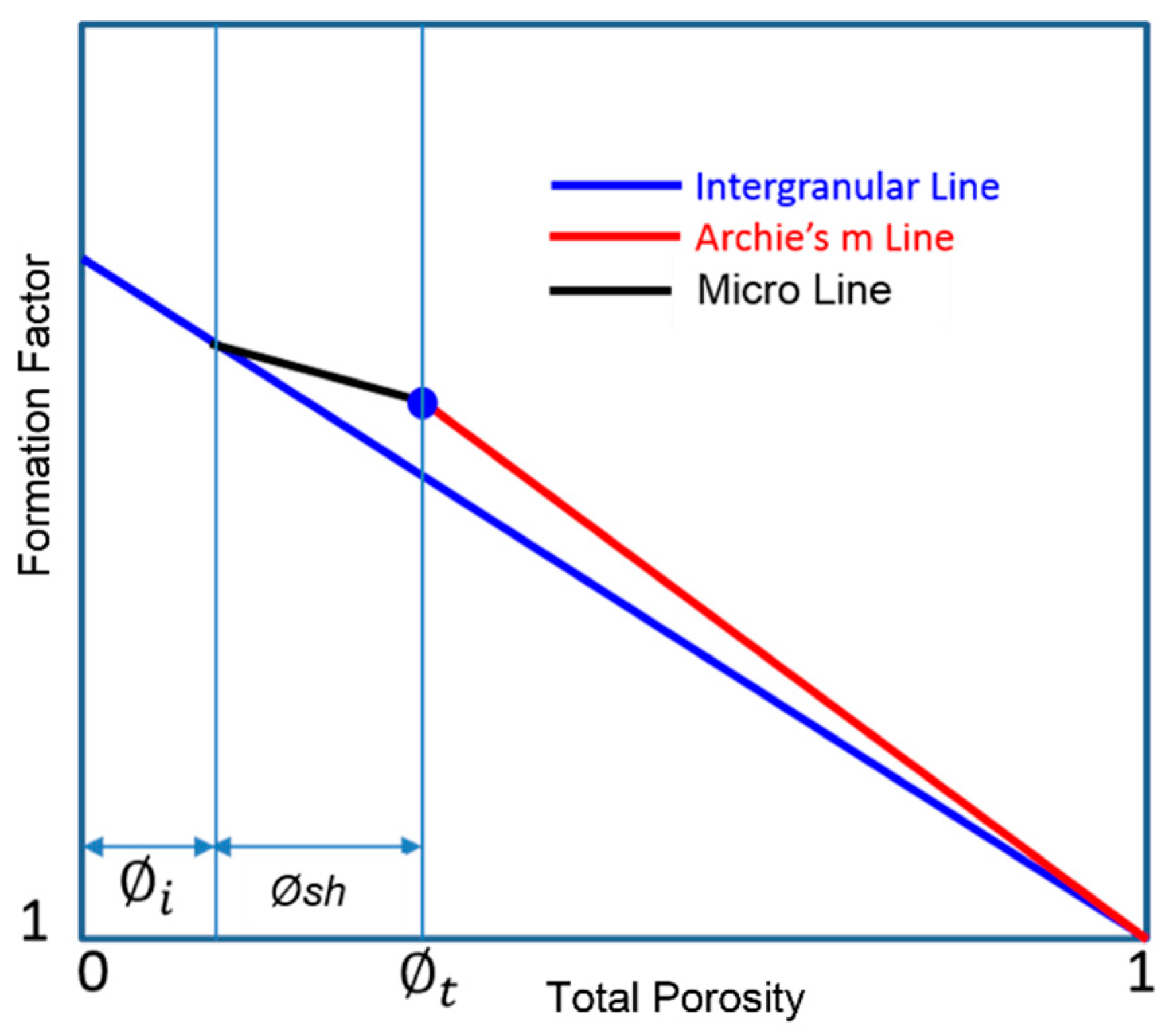
where ${\lambda }_s$ is the lithology exponent for intergranular pores and ${\lambda }_{sh}$ is the lithology exponent for micropores. $F$ is the ratio of the resistivity of 100% water-saturated rock to brine resistivity, called the formation factor. Figure 1 represents the PCM methodology for a dual-pore sandstone formation.

As explained in Shahin et al. [20], the intergranular pore and micropore lithology exponents can be obtained from the nonlinear optimization of resistivity core measurements. In the following, we will present a new methodology to obtain these parameters from conventional well logs.

With the same notation used by Shahin et al. [17], the formation factor ($F$) and total porosity, i.e., $F$-${\varphi }_t$ are plotted in the log–log plane. Starting from point ($F$ = 1 and ${\varphi }_t$ = 1), a line with slope of ${\lambda }_s$ illustrates the gradual decrease in total porosity due to sediment compaction. At this stage, intergranular pores are the only pore system and total porosity (${\varphi }_t$) is equal to intergranular porosity of ${\varphi }_s$. Then, diagenesis comes into play and micropores begin to evolve. A line with slope ${\lambda }_{sh}$ represents the evolution of the microporosity ${\varphi }_{sh}$. This line has a different slope than the line of intergranular pores. When the diagenesis process is finished, the sample has a total porosity of ${\varphi }_t$, which is the summation of ${\varphi }_{sh} \mathrm{and} {\varphi }_i.$ The line connecting the final position of sample in the $F$-${\varphi }_t$ plane with the point of ($F$ = 1, ${\varphi }_t$ = 1) is Archie’s line with slope m, which represents the lithology exponent [17].

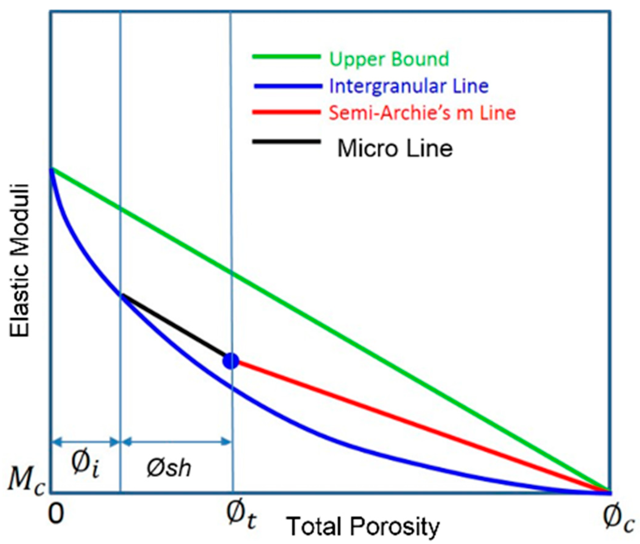
6. Elastic Modeling Using Staged Differential Effective Medium (SDEM)

Reuss lower bound and Voight upper bound have been utilized historically to associate the elastic moduli of rock components with the elastic moduli of the mixture. While the moduli of the mixtures are always located between these bounds [21], several researchers attempted to better locate moduli exact positions by adding more textural information on how grains and pores are structured within the rocks. One such attempt was the work by Myers and Hathon [3], which extended the differential effective medium theory by introducing the concept of “staging” on how the process of sedimentation, lithification/compaction, and diagenesis combine to form sedimentary rocks. In the staged differential effective medium (SDEM) technique, inclusions of different length scale (aspect ratio) are gradually added to a host, neglecting interaction terms between the inclusions [20].

Similar to PCM to model resistivity, SDEM methodology models the elastic moduli of dual-porosity sandstones. In fact, PCM is a special case of SDEM, and these are general techniques for modeling the effect of mineralogy and texture on permeability, resistivity, and elastic measurements.

The well-known critical porosity [22] model is inherently included in SDEM. To simulate the elastic moduli of a single-pore sandstone, we need a two-staged SDEM. The first step is to integrate the elastic moduli from host to the critical porosity with a length scale of L = 0, which mimics an isostress Reuss bound. The second step is to integrate from critical porosity to total porosity with a length scale of L#0 using:

$$M=M_c\frac{1+\left(\frac{{\varnothing }_c-\varnothing }{{\varnothing }_c}\right).\left(\frac{M_i-M_c}{M_c}\right).L}{1-\left(\frac{{\varnothing }_c-\varnothing }{{\varnothing }_c}\right).\left(\frac{M_i-M_c}{M_i}\right).\left(1-L\right)}$$

(7)

where ${\varnothing }_c$ is the critical porosity, $M_i$ is the inclusion modulus, $L$ is the length scale and related to this inclusion, and $M_c$ is the isostress bound of the host and grain modulus at the critical porosity [20].

Dual-porosity sandstone can be simulated by adding an additional integration step to model the micropores [3]. Figure 2 illustrates the SDEM technique for a dual-porosity formation. The elastic moduli (bulk and shear) are plotted versus total porosity (${\varphi }_t$). The bound corresponding to length scale of $L_s$ connects the elastic moduli at critical porosity ($M_c$) to elastic moduli at zero porosity (solid or matrix moduli). This bound is associated with intergranular pores. The bound corresponding to length scale of $L_{sh}$, which does not pass through elastic moduli at critical porosity, is associated with the moduli change due to change in microporosity. For a formation consisting of intergranular pores and micropores, the microporosity bound intersects the intergranular bound at the intergranular porosity.

As explained in Shahin et al. [20], matrix elastic moduli, critical porosity, intergranular pore and micropore $L$ parameters, and lithology exponents of each pore system can be obtained from the nonlinear optimization of velocity and resistivity core measurements. In the following, we present a new methodology to obtain these parameters from conventional well logs.

The elastic moduli of the mixture ($M$) and total porosity, i.e., $M$-${\varphi }_t$ are plotted in a linear plane; ${\varphi }_i$ is the intergranular porosity, ${\varphi }_m$ is the microporosity, and the sum ${\varphi }_t={\varphi }_{i+}{\varphi }_m$, is the total porosity. Starting from point (${\varphi }_C, M_c$) a bound with length scale of $L_i$ illustrates the gradual decrease in total porosity due to sediment compaction. At this stage, intergranular pores are the only pore system and total porosity (${\varphi }_t$) equal to intergranular porosity of ${\varphi }_i$. Then, diagenesis comes into play and micropores start to evolve. A bound with length scale of $L_m$ represents the evolving of the microporosity of ${\varphi }_m$. This bound has a different length scale than the bound of intergranular pores. When the diagenesis process is finished, the sample has a total porosity of ${\varphi }_t$, which is the summation of ${\varphi }_m \mathrm{and} {\varphi }_t$. The bound connecting the final position of sample in $M$-${\varphi }_t$ plane with the point of (${\varphi }_C, M_c$) is the semi-Archie’s line described in Figure 1.

7. Multiphysics Modeling to Construct Dual-Porosity Sandstones

As mentioned earlier, PCM is a special case of SDEM, and these are general techniques for modeling the effect of mineralogy and texture on permeability, resistivity, and elastic measurements. On core scale measurements of resistivity and velocities, PCM and SDEM have been found satisfactory to model pore structure of dual-porosity carbonates [20]. They made three independent porosity measurements (Archimedes, µCT, and NMR) on twelve carbonate core plugs from the northern Niagaran reef. They modeled two pore types, micropore and vugs. Resistivity, P- and S-wave ultrasonic measurement of the same brine saturated core plugs were made. The joint modeling of resistivity and velocities was performed using PCM and SDEM techniques. The parameters in the resistivity and velocity models were optimized using the VFSA algorithm [5,23]. The optimization algorithm was able to fine tune the model parameters of resistivity and velocities to provide vuggy and microporosities close to independently measured porosities using NMR and µCT. In this paper, we extend this technique from core data to well logs and demonstrate it using constructed logs from an actual carbonate formation.

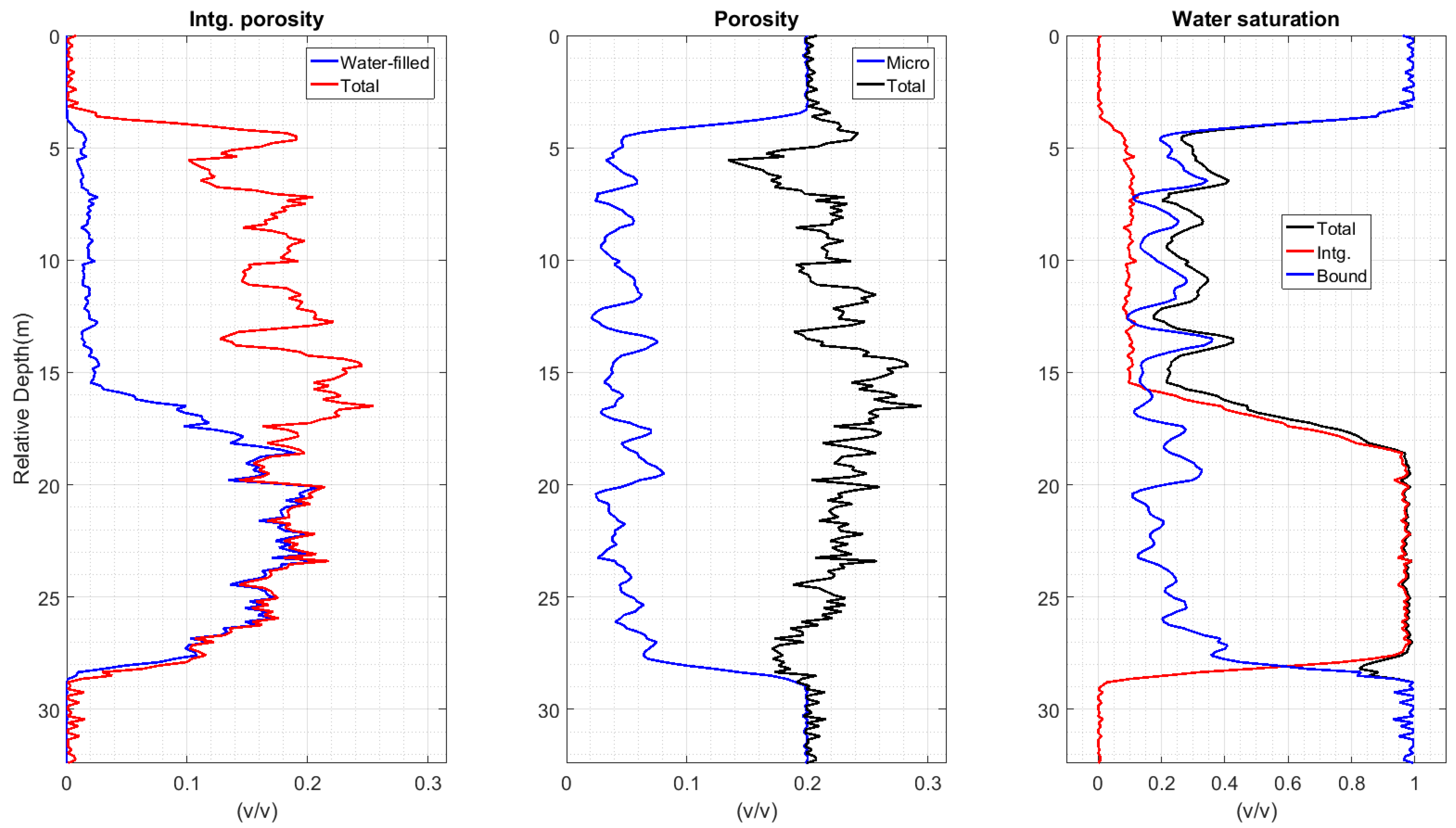
Figure 3 illustrates dual-pore shaly sandstone with 24 m thickness that is partially saturated with oil in the upper 10 m of the formation. The residual water saturation in the upper portion is about 3%. The lower 9 m is fully water saturated. The middle (~4 m) is the transition zone. The salinity of the formation water is 120 Kppm. To model the density log, quartz with density (g/cm³) of 2.65, feldspar of 2.52, illite of 2.52, brine of 1.05, and oil with density of 0.75 are used. To replicate gamma-ray responses, gamma-ray values of 0.0, 220, and 275 API are considered for quartz, feldspar, and illite, respectively. To simulate the resistivity using PCM, the lithology exponents of shale and sandstone are assumed to be 0.75 and 1.75, respectively. Temperature is 60 degrees Celsius. P- and S-wave slowness (sonic travel times) is modeled using SDEM. Bulk moduli (in GPa) are set to 37, 29, and 25 for quartz, feldspar, and illite, respectively. Shear moduli (in GPa) are set to 44, 15, and 16 for quartz, feldspar, and illite, respectively. Bulk moduli (in GPa) are set to 2.5 and 0.75 for brine and oil, respectively. The critical porosity is 0.45. Length scales for shale and sandstone are set to 1.0 and 0.2, respectively.

In the first track from the left, intergranular porosity is displayed in red and water-filled intergranular porosity is shown in blue. In the middle track, total porosity is in black and microporosity is in blue. In the right track, total, intergranular, and bound water saturations are shown in black, red, and blue, respectively.

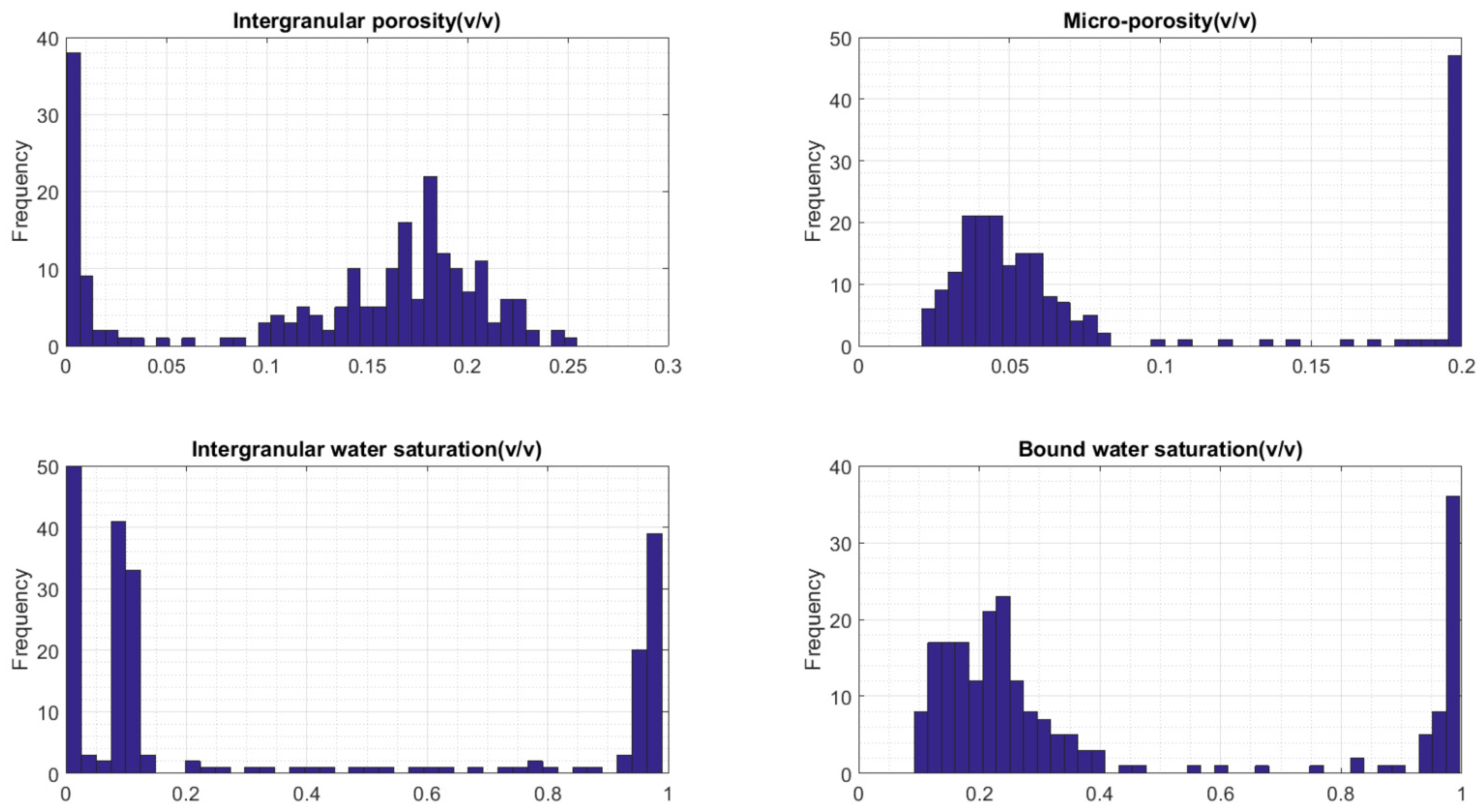
Figure 4 displays the histograms of the true petrophysical properties including intergranular porosity, microporosity, intergranular water saturation, and micropore water saturation.

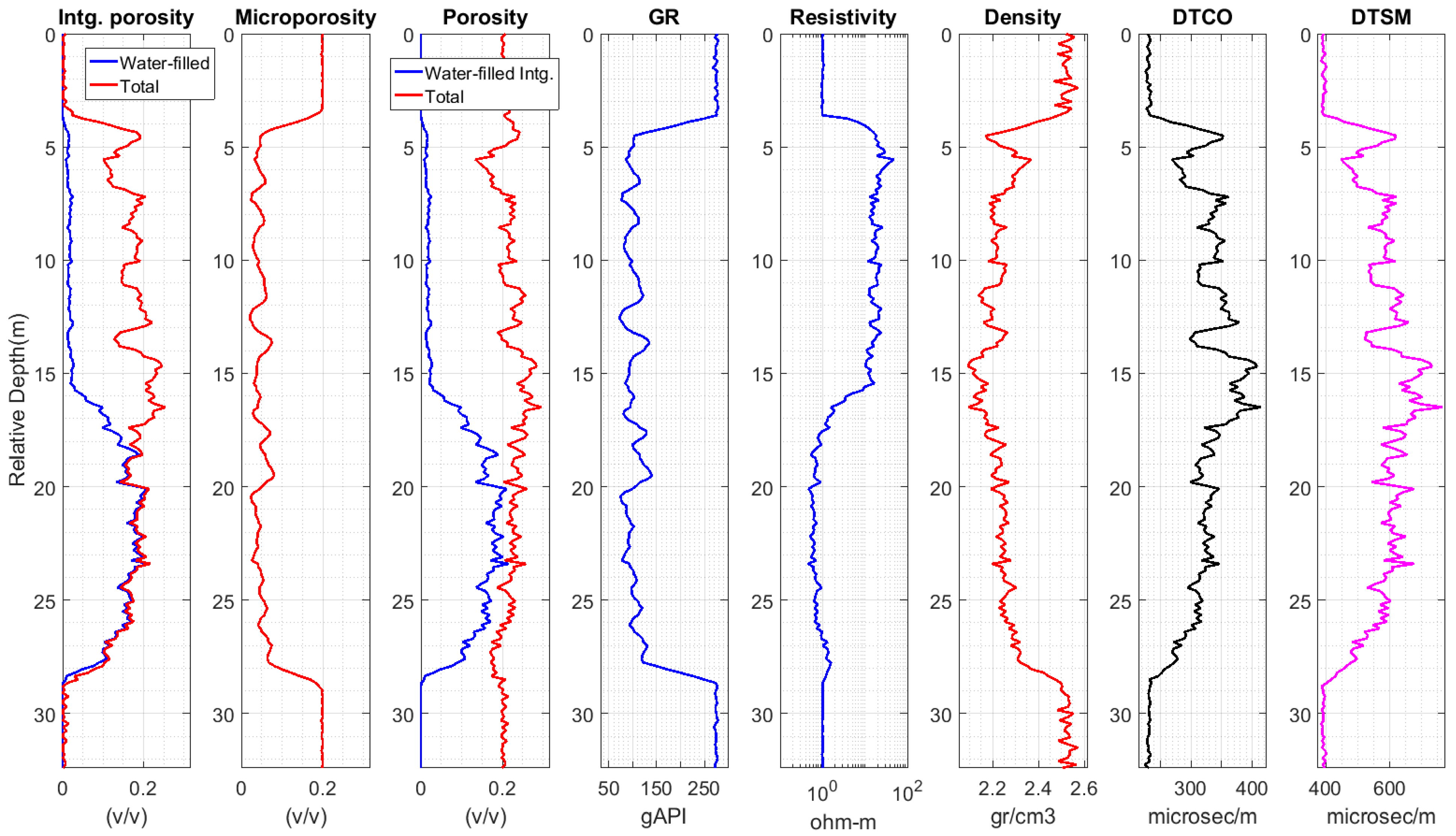
Figure 5 displays the simulated well-log responses over the dual-porosity sandstone formation shown in Figure 3. Bulk density (${\rho }_b$) is modeled using mass conservation, P-wave slowness (DTCO) and S-wave slowness (DTSM), modeled using SDEM, and electrical resistivity ($R_t$) using PCM. Model parameters are summarized in

Table 1. Reservoir, matrix, fluid, and model parameters for the dual-porosity sandstone formation.

Properties	Symbol	Values	Units
Reservoir thickness	h	24.00	meter
Reservoir temperature	T	60.00	°C
Irreducible water saturation	$S_{wirr}$	0.10	Fractional
Residual oil saturation	$S_{or}$	0.03	Fractional
Salinity	Sal	120.00	Kppm
Quartz density	${\rho }_Q$	2.65	g/cm3
Feldspar (orthoclase) density	${\rho }_{Fd}$	2.52	g/cm3
Clay (illite) density	${\rho }_{sh}$	2.52	g/cm3
Brine density	${\rho }_w$	1.05	g/cm3
Oil density	${\rho }_o$	0.75	g/cm3
Quartz bulk modulus	$K_Q$	37.00	GPa
Feldspar bulk modulus	$K_{Fd}$	29.00	GPa
Quartz shear modulus	${\mu }_Q$	44.00	GPa
Feldspar shear modulus	${\mu }_{Fd}$	15.00	GPa
Clay bulk modulus	$K_{sh}$	25.35	GPa
Clay shear modulus	${\mu }_{sh}$	16.26	GPa
Clay gamma ray	$G{R}_{sh}$	275.00	API
Quartz gamma ray	$G{R}_Q$	0.00	API
Feldspar gamma ray	$G{R}_{Fd}$	220.00	API
Brine bulk modulus	$K_w$	2.50	GPa
Oil bulk modulus	$K_o$	0.75	GPa
Critical porosity	${\varnothing }_c$	0.45	Fractional
Micropore lithology exponent	${\lambda }_m$	0.75	Fractional
Intergranular lithology exponent	${\lambda }_i$	1.75	Fractional
Micropore length scale for bulk modulus	$L_m^k$	1.00	Fractional
Intergranular length scale for bulk modulus	$L_i^k$	0.20	Fractional
Micropore length scale for shear modulus	$L_m^{\mu }$	1.00	Fractional
Intergranular length scale for shear modulus	$L_i^{\mu }$	0.20	Fractional

. As expected, distinct fluid zones are clearly separated on the resistivity log in logarithmic scale and one can determine oil column, transition zone, and water leg from reservoir top to bottom, respectively. This trend can be seen on density and sonic logs in some degree, but it is not as clear as the resistivity log due to the higher combination effect of porosity and saturation on sonic and density logs.

From left to right, the first three tracks show the basic petrophysical properties already discussed in the previous figures. The fourth track displays the gamma-ray (GR) response simulated by the volumetric equation for the reservoir and surrounding shales. The fifth track is electrical resistivity replicated with PCM. The sixth track is bulk density expressed by mass conservation, and the seventh and eighth tracks are compressional (P-wave) and shear (S-wave) slowness simulated with SDEM.

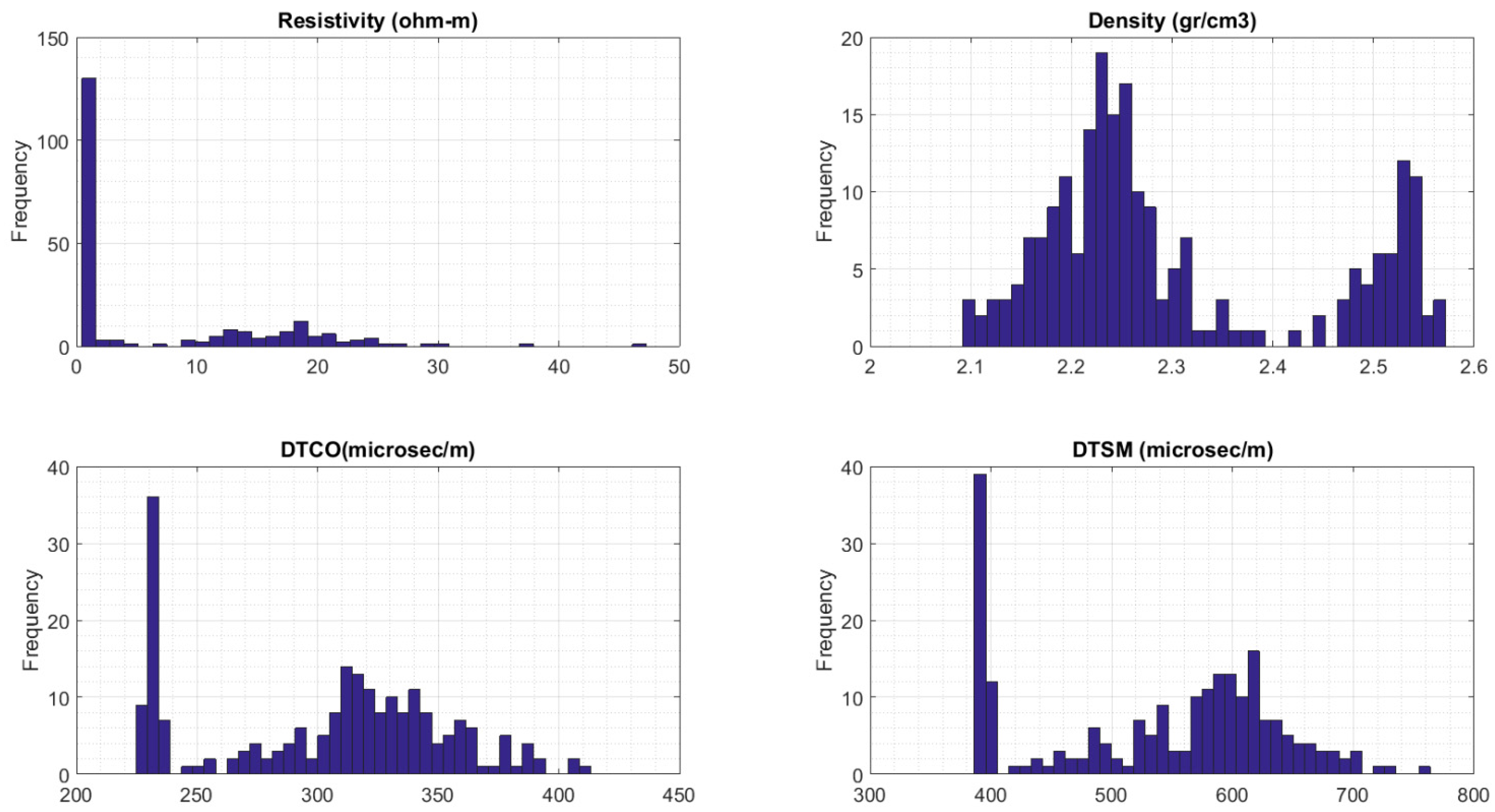
Figure 6 displays the histograms of the well-log responses simulated using multiphysics models. As expected, fluid zones are separated on the resistivity histogram in linear scale and one can distinguish the oil column from water leg in some degree. This separation cannot be seen on density and sonic histograms because of the higher combination effect of porosity and saturation on sonic and density logs.

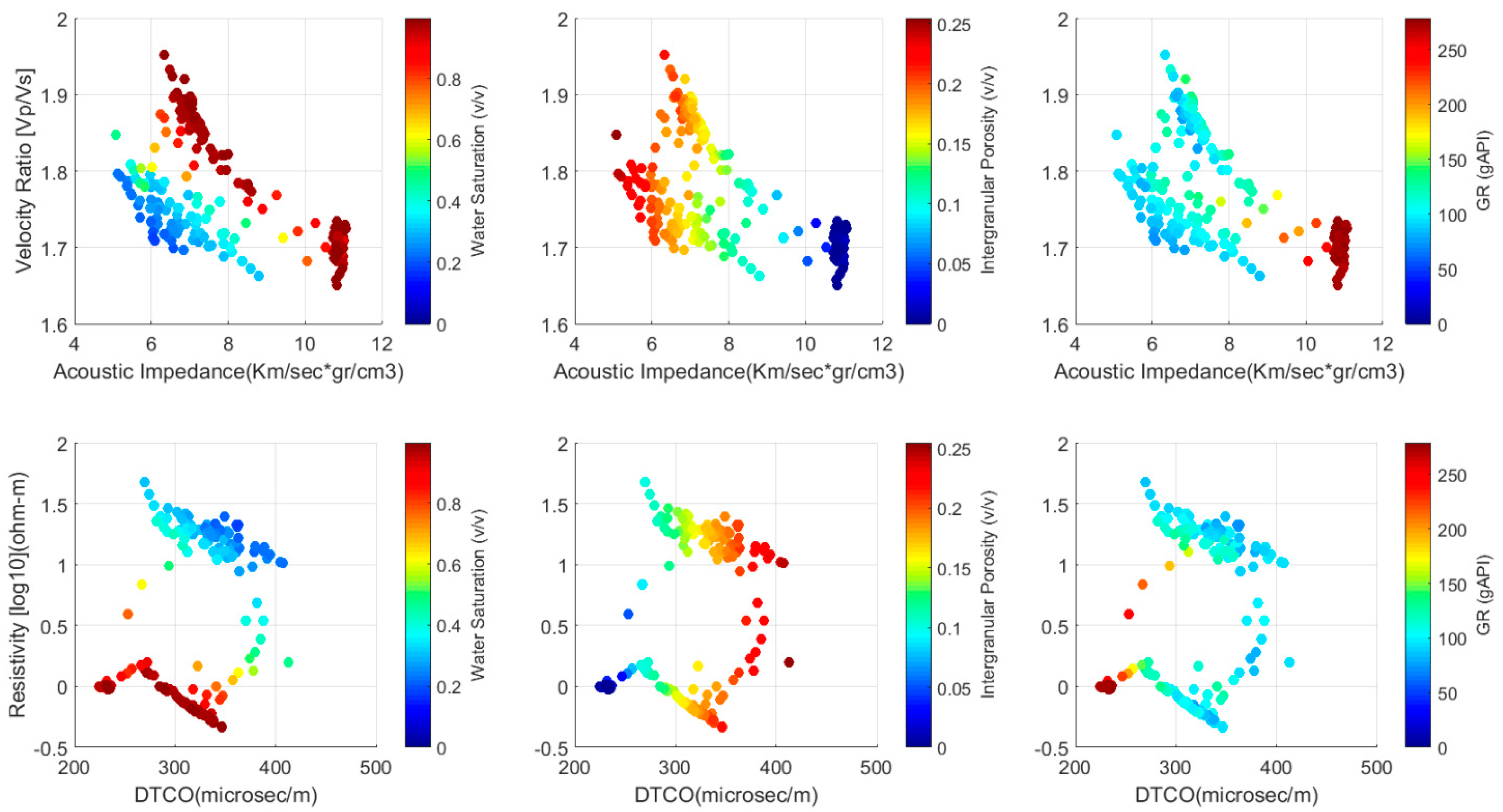
Figure 7 displays cross-plots of resistivity and elastic properties (slowness, velocity, acoustic impedance, and velocity ratio). Multiphysics rock templates of this kind help interpreters to identify and separate litho–fluid facies. We intentionally utilize two different rock templates in this figure.

The first type of template is mainly derived from seismic attributes including velocity ratio, i.e., the ratio of P-wave velocity to S-wave velocity, and acoustic impedance, i.e., P-wave velocity multiplied by density. These types of templates help seismic analysts to interpret seismic inversion results. For example, from the top left panel in this figure, one can conclude that oil-bearing and water-bearing zones can be separated using velocity ratio and acoustic impedance seismic attributes where all the points are color-coded by water saturation. From the top right panel in this figure, one can clearly see the gradual effect of intergranular porosity on velocity ratio and acoustic impedance seismic attributes where all the points are color-coded by intergranular porosity.

The second type of template is mainly derived from petrophysical properties including resistivity and compressional slowness (DTCO). These types of templates help petrophysicists to interpret well logs. For example, from the bottom left panel in this figure, one can conclude that oil-bearing and water-bearing zones can be separated using resistivity and DTCO well logs where all the points are color-coded by water saturation. From the bottom right panel in this figure, one can clearly see the gradual effect of intergranular porosity on resistivity and DTCO well logs where all the points are color-coded by intergranular porosity.

8. Stochastic Inversion Algorithm to Decipher Dual-Porosity Sandstones

As implemented by Shahin et al. [17], we utilize the same optimization engine (VFSA) to minimize the objective function (see Appendix A and Appendix B for details). In this paper, an objective function is defined as the root mean square of differences between simulated and observed well logs including density, resistivity, and P- and S-wave slowness logs (DTCO and DTSM). Two sets of parameters are defined in the optimization workflow.

Global parameters consist of matrix density, matrix bulk and shear moduli, salinity, critical porosity, intergranular lithology exponent for resistivity, and intergranular L parameter (length scales) for bulk and shear moduli. Global parameters remain constant over the depth interval of interest. The micropore lithology exponent for resistivity is set to 0.75 based on previously published results [3]. Micropore L parameters for bulk and shear moduli are set to 1.0 based on the previously published results [3]. In VFSA optimization structure, we evaluate the global error function to update the global model parameters.

Local model parameters changing as functions of depth include intergranular porosity (${\phi }_i$), microporosity (${\phi }_m$), total porosity (${\phi }_t$), and water saturation ($S_w$) at each depth interval. In VFSA structure, we evaluate the local error function to update the local model parameters in the corresponding depth interval.

We design an objective function that has four terms. The first term is the difference between bulk density well-log data (${\rho }_b^{obs.}$) and modeled bulk density (${\rho }_b^{sim.}$) using the mass balance equations. The second term is the difference between resistivity well-log data ($R^{obs.}$) and modeled resistivity ($R^{sim.}$) using the PCM methodology. The third and fourth terms are the difference between DTCO and DTSM well-log measurements ($DTC{O}^{obs.}$ and $DTS{M}^{obs.}$) and their corresponding simulated logs using the SDEM model ($DTC{O}^{Sim.}$ and $DTS{M}^{Sim.}$). Note that all the terms are normalized to the summation of well-log observations and simulated well-log responses. This will facilitate the quality control of error (objective or cost) function.

$$\begin{array}{c}\mathsf{\Delta }E=\frac{{{\displaystyle \sum }}_{i=1}^n{\left({\rho }_b^{sim.}-{\rho }_b^{obs.}\right)}^2}{{{\displaystyle \sum }}_{i=1}^n{\left({\rho }_b^{sim.}+{\rho }_b^{obs.}\right)}^2}+\frac{{{\displaystyle \sum }}_{i=1}^n{\left(R^{sim.}-R^{obs.}\right)}^2}{{{\displaystyle \sum }}_{i=1}^n{\left(R^{sim.}+R^{obs.}\right)}^2}+\frac{{{\displaystyle \sum }}_{i=1}^n{\left(DTC{O}^{sim.}-DTC{O}^{obs.}\right)}^2}{{{\displaystyle \sum }}_{i=1}^n{\left(DTC{O}^{sim.}+DTC{O}^{obs.}\right)}^2}\\ \hspace{1em}\hspace{1em}\hspace{1em}\hspace{1em}\hspace{1em} +\frac{{{\displaystyle \sum }}_{i=1}^n{\left(DTS{M}^{sim.}-DTS{M}^{obs.}\right)}^2}{{{\displaystyle \sum }}_{i=1}^n{\left(DTS{M}^{sim.}+DTS{M}^{obs.}\right)}^2}\end{array}$$

(8)

To converge the VFSA optimization and to obtain meaningful physical model parameters, we apply several constraints. Some of the important ones follow:

• In each depth interval, the microporosity and intergranular porosities are smaller or equal to given total porosities.

$${\phi }_i\le {\phi }_t$$

(9)

$${\phi }_m\le {\phi }_t$$

(10)

2.

In each depth interval, the sum of microporosity and intergranular porosity should be equal to total porosities.

$${\phi }_i+{\phi }_m={\phi }_t$$

(11)

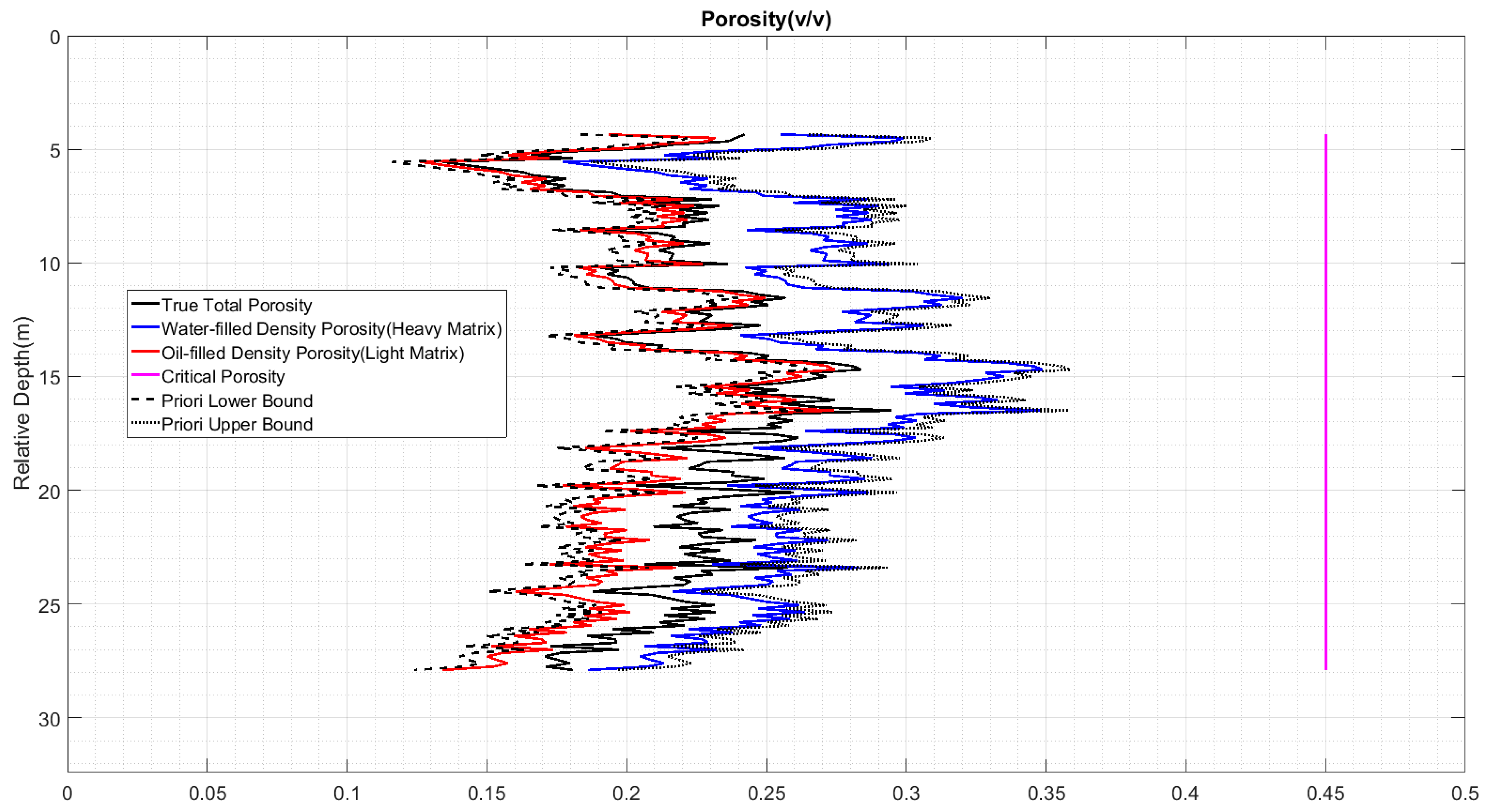
3.

The lower search bounds on total porosity are computed from the density log. Initial upper and lower bounds are first computed using a heavy mixture (heavy grain and water) and a light mixture (light grain and hydrocarbon), respectively. Then, safety factors in percentage are added to and subtracted from initial upper and lower bounds, respectively, to form conservative search bounds (Figure 8).

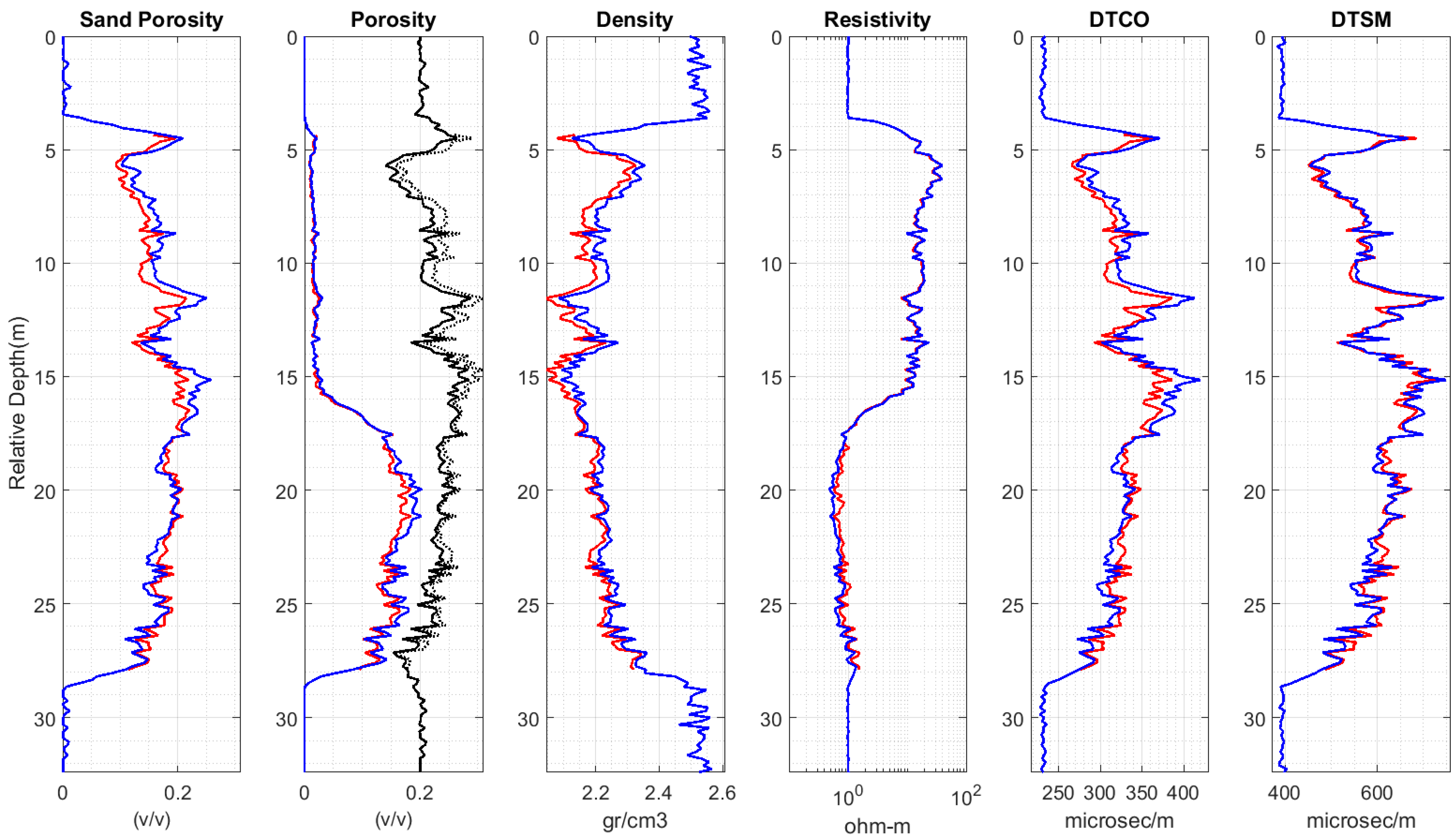
In Figure 9, a single realization of true and inverted petrophysical properties and associated well-log responses are overlaid in different panels. The inversion workflow is capable of matching the data for the three portions of carbonate formation (oil column, water leg, and transition zone) and retrieving intergranular, micro, total, and water-filled porosities with high precision.

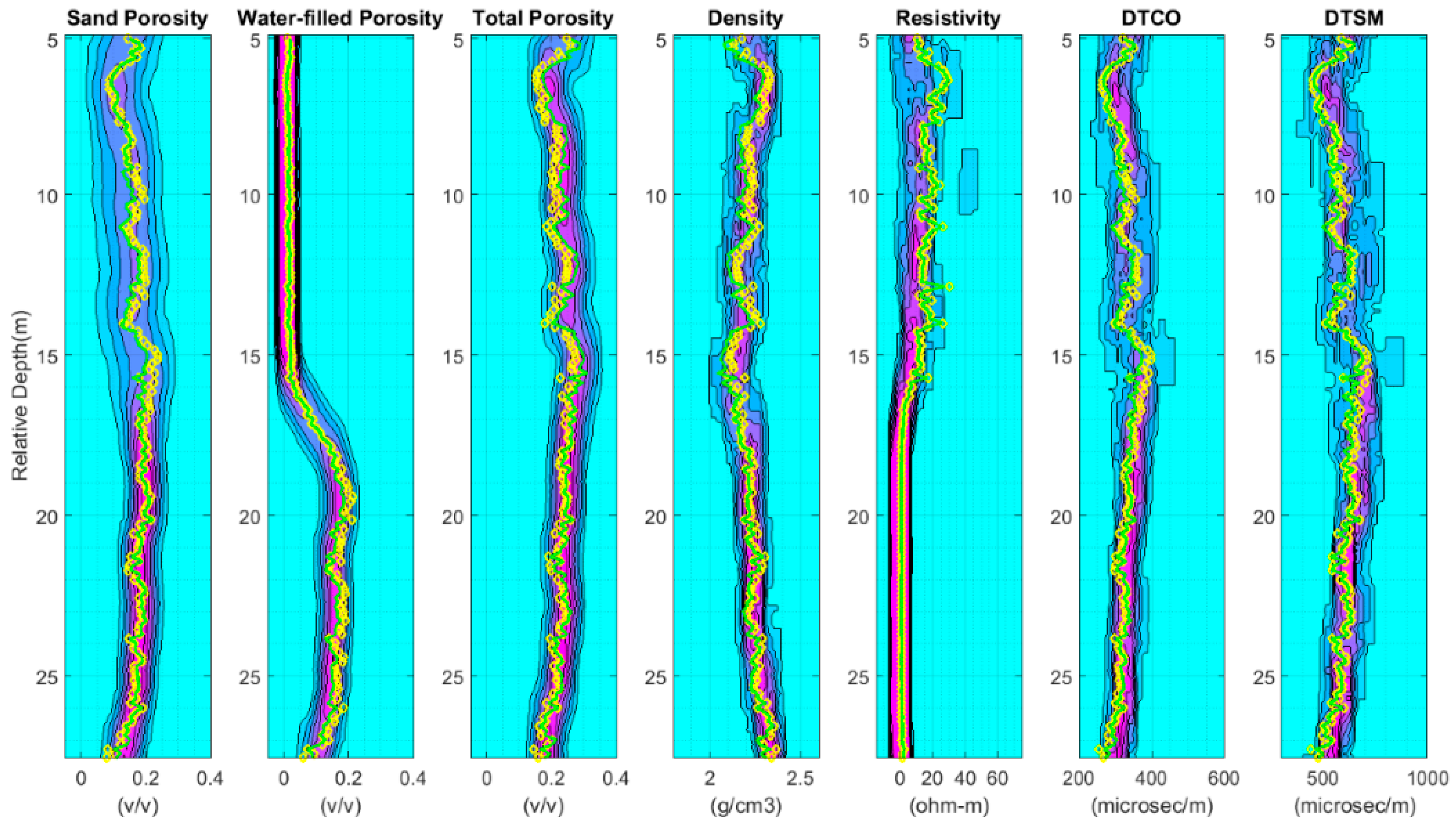
In Figure 10, true and inverted petrophysical properties and associated well-log responses are overlaid in all panels for 100 realizations. Note that the mean of 100 independent realizations are very close to true petrophysical properties and associated well-log responses. The inversion workflow is capable of matching the data for the three portions of carbonate formation (oil column, water leg, and transition zone) and retrieving intergranular, micro, total, and water-filled porosities with high precision.

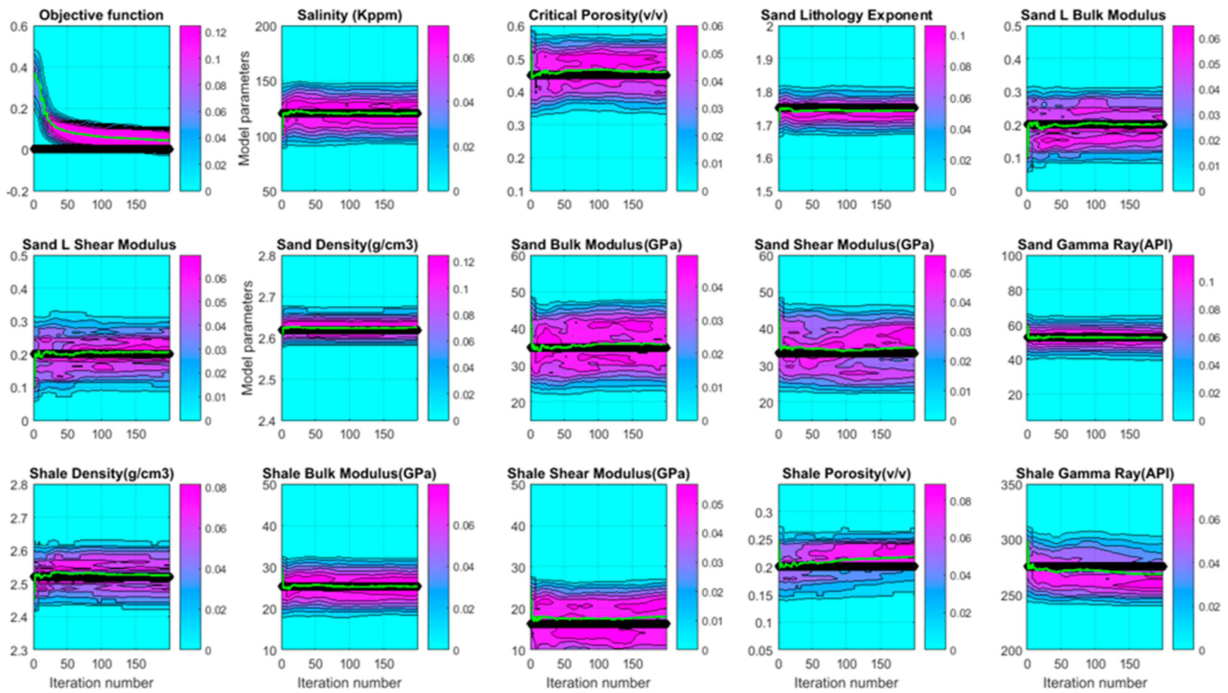
Figure 11 shows the performance of inversion workflow to recover global parameters by minimizing the normalized objective function. Note that the mean value of 100 realizations is close to the true value of each global parameter.

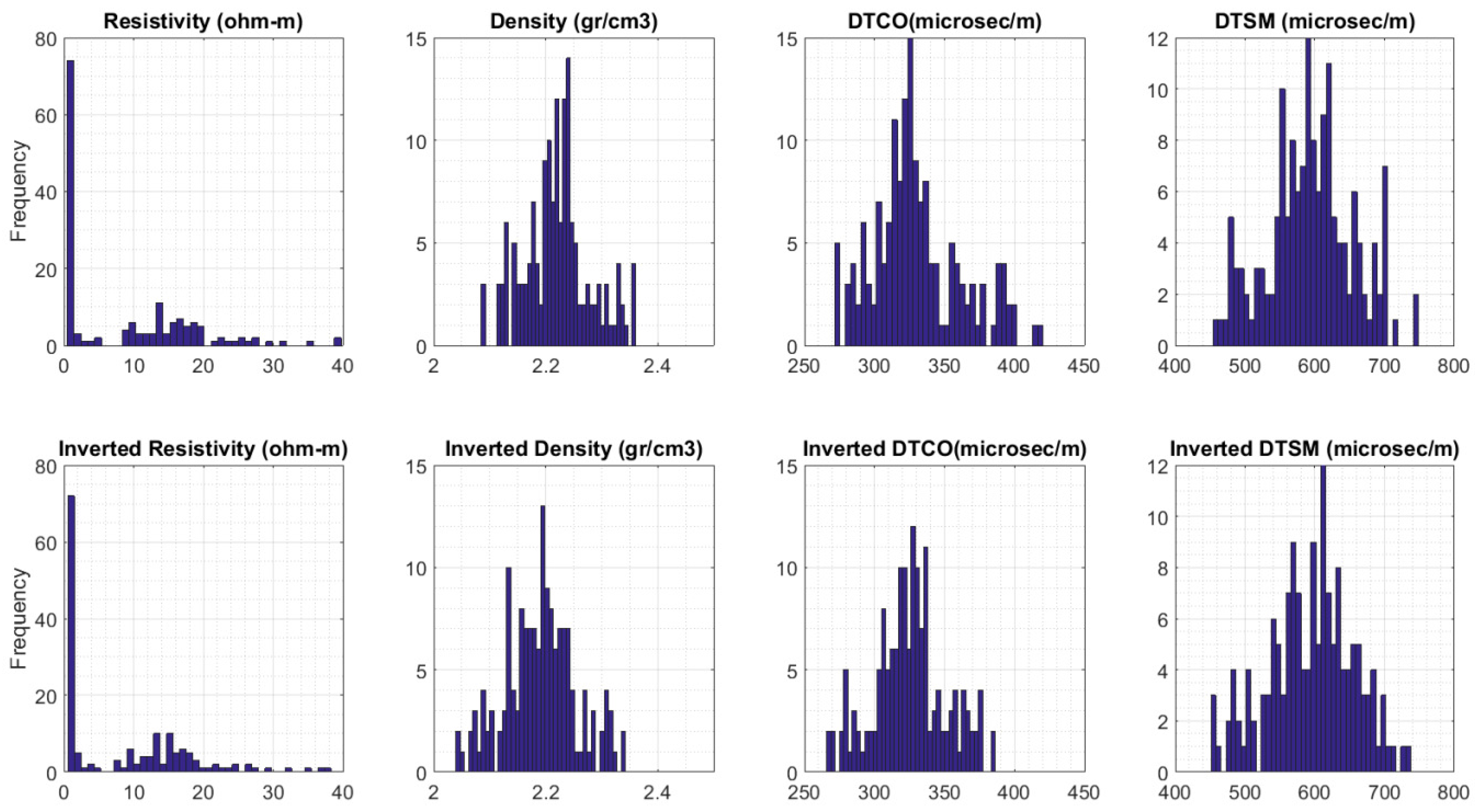
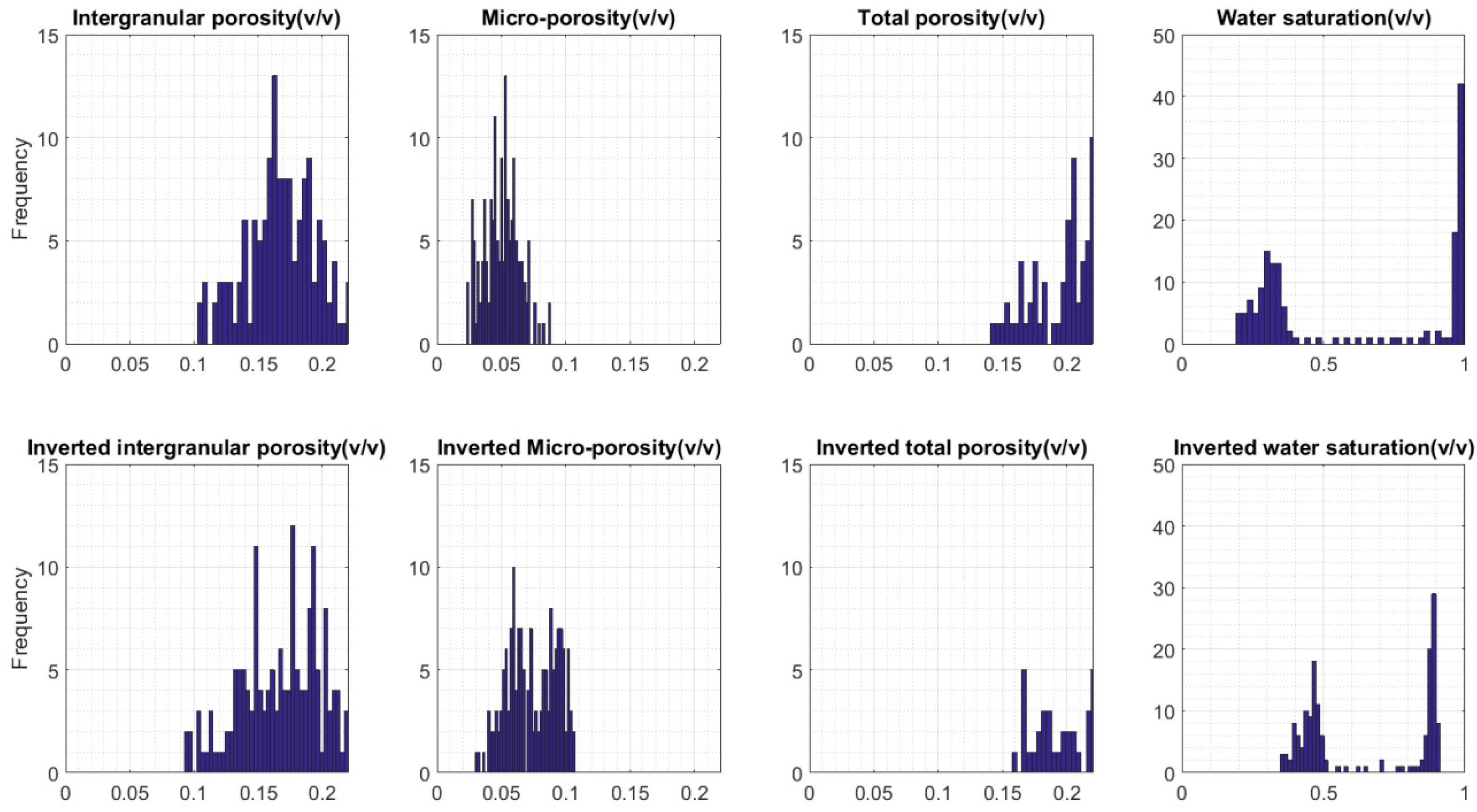
Figure 12 demonstrates the histograms of the true petrophysical properties and their inverted values. The distributions of true and inverted properties are very similar and that implies the inversion algorithm not only estimates the petrophysical properties with high precision, but also preserves the statistics of the true properties.

Figure 13 displays the histograms of the true well-log responses and their inverted values. The distributions of true and inverted well-log responses are very similar and that implies the inversion algorithm not only replicates the true well-log responses with high precision, but also preserves the statistics of the true responses.

9. Discussion

Very often rock physics modeling and formation evaluation are treated as independent tasks. This is attributed to several causes: lack of communication between petrophysicists and seismic analysts (organizational silos), insistence on using simple linear or quasilinear models in well-log interpretation, and lack of core and fluid samples to provide calibrated rock matrix and fluid properties, salinity, critical porosity, Archie’s parameters, etc.

The joint inversion algorithm customized here utilizes an iterative global optimization machine (Appendix A). A particular type of simulated annealing is designed enabling simultaneous recovery of global and local model parameters and their associated uncertainties (Appendix B). The iteration number in VFSA has the same effect as regularization in other well-known inversion algorithms including Thikhonov regularization and singular value decomposition [24,25]. To emphasize the main disadvantages of the proposed workflow, we should confirm that the VFSA optimization is relatively slow and computing cost is high. To overcome this issue, one should employ multiphysics models to rapidly simulate well-log responses.

We observe that simulated well-log responses match very well with true well logs (Figure 9). We also find that resistivity is the best resolved well-log response. Sonic slowness logs (DTCO and DTSM) are reasonably recovered but not as good as resistivity. Density is well recovered in the oil column and transition zone, but inverted density has a negative shift from true density in the water leg. The same shifts, but positive and milder, are also observed in DTCO and DTSM logs leading to underestimating water saturation in the water leg (Figure 12). Total porosity is the best resolved parameter. Intergranular porosity and microporosity are the next resolved parameters. Water saturation is reasonably recovered, but not as well as other properties, especially in the water leg as explained above. Salinity is the best resolved global parameter. Other global parameters are recovered but not as well as salinity, especially matrix properties (Figure 11).

It is worth noting that the accuracy and resolution of the inverted petrophysical properties depend on the tools’ depth of investigation, tools’ vertical resolution, reservoir thickness, and the invasion profile in the formation. To account for these concerns, one needs to include detailed modeling of the resistivity, density, and sonic tools, and a realistic invasion profile. In this work, we ignore the invasion profile by assuming negligible or complete invaded zone. We anticipate that our inversion workflow works best for relatively thick sandstone formations. While the stochastic component of the proposed inversion workflow is supposed to recover high-resolution petrophysical properties, it is recommended to consider detailed modeling of well-logging tools to accurately simulate shoulder-bed effects for laminated and thin bed sandstones. We further assume the formation of interest is a sandstone with mineralogy remaining constant in reservoir interval. That means a single matrix density properly represents the entire interval. If it is not the case, one may want to divide reservoir interval into several isolithologic units and apply the inversion workflow independently for each unit. The other alternative is to use gamma ray (GR), photoelectric (PEF), and neutron porosity well logs to help differentiate lithologic units. In the ideal case, our workflow can be extended to invert for volumetric fraction of minerals together with pore type, porosity, and fluid saturations.

10. Conclusions

An integrated multiphysics technique is proposed to jointly model the resistivity, density, and elastic responses of dual-pore sandstones. We construct the well-log responses using the multiphysics model. We then design a customized VFSA search engine to perform a novel inversion workflow. Matrix properties (density and elastic moduli), salinity, critical porosity, PCM–SDEM model parameters, intergranular porosity, microporosity, total porosity, and water saturation are the main properties estimated via this inversion algorithm. In the proposed workflow, one can seamlessly quantify the uncertainty of global and local model parameters.

Our future work is to extend this methodology by including other logs (GR, neutron, PEF, EPT, and NMR). By doing so, we will estimate the volumetric fraction of minerals, pore type, porosity, saturation, matrix properties, salinity, critical porosity, resistivity lithology exponents, and sonic length scales for different pore networks. The current workflow only considers the case with no radial dependence of the formation water salinity. Future work will also extend the current workflow to cases including the effects of invasion. The next logical step is to use this calibrated multiphysics model to invert prestack seismic data back to mineralogy, pore type, porosity, and saturation.