
Concatenated Network Fusion Algorithm (CNFA) Based on Deep Learning: Improving the Detection Accuracy of Surface Defects for Ceramic Tile


Abstract
:1. Introduction
2. Methodology
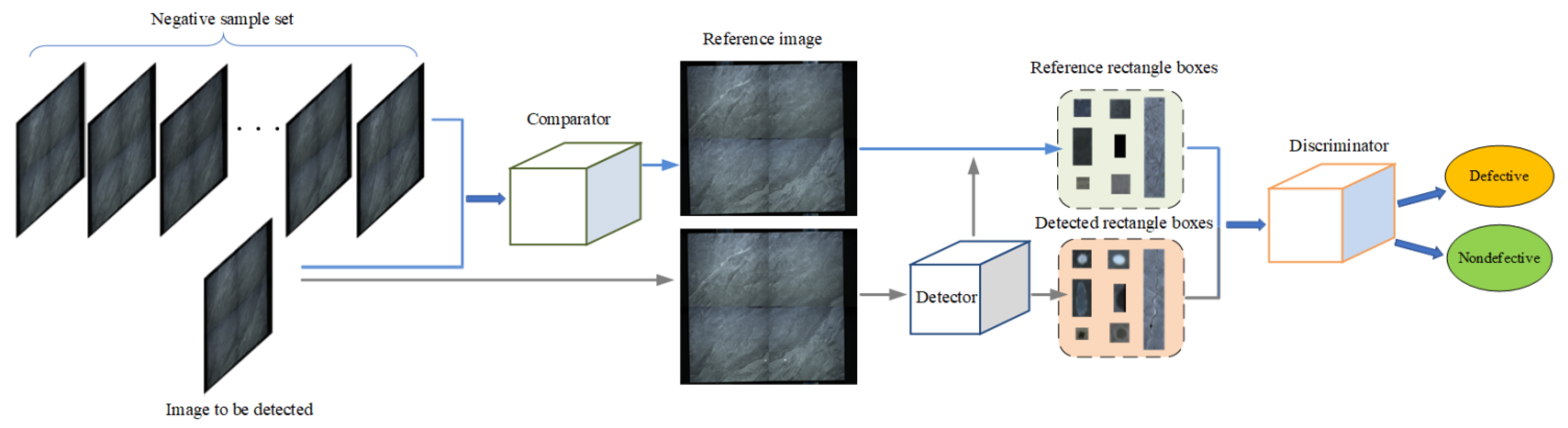
2.1. Architecture and Workflow
2.2. Comparator
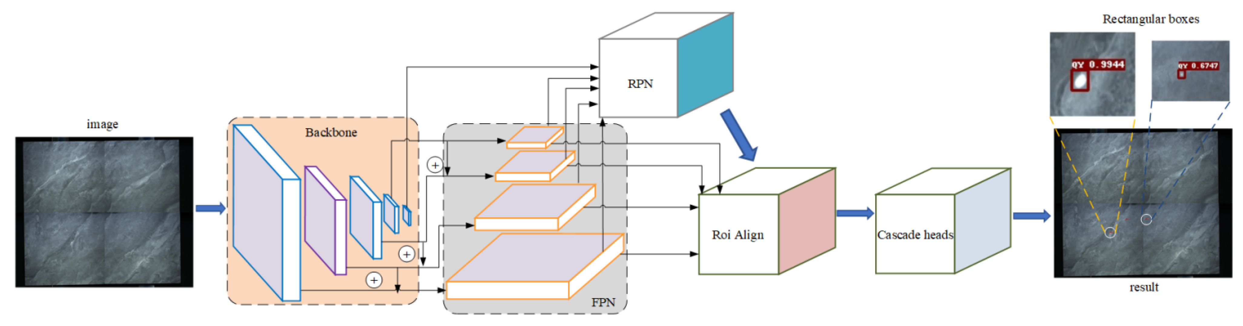
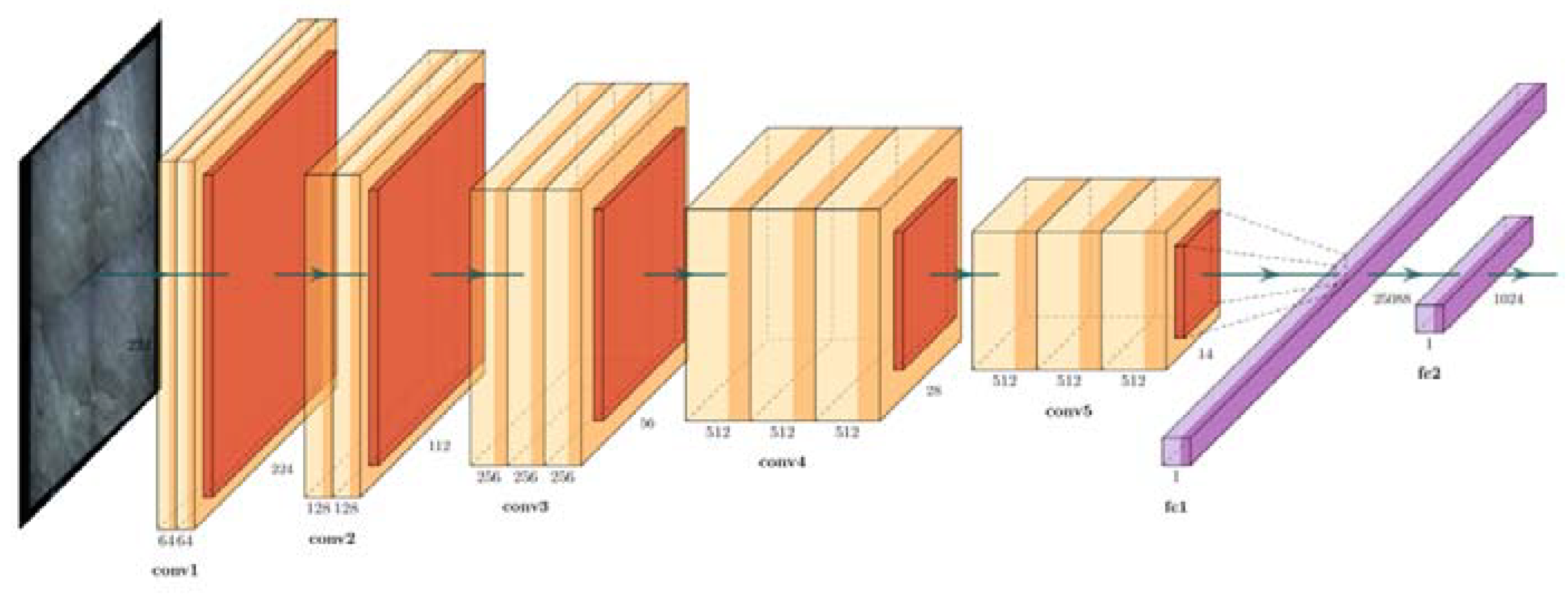
2.3. Detector
2.4. Discriminator
3. Experiments
3.1. Datasets
3.2. Experimental Configuration
3.3. Evaluation Methodology
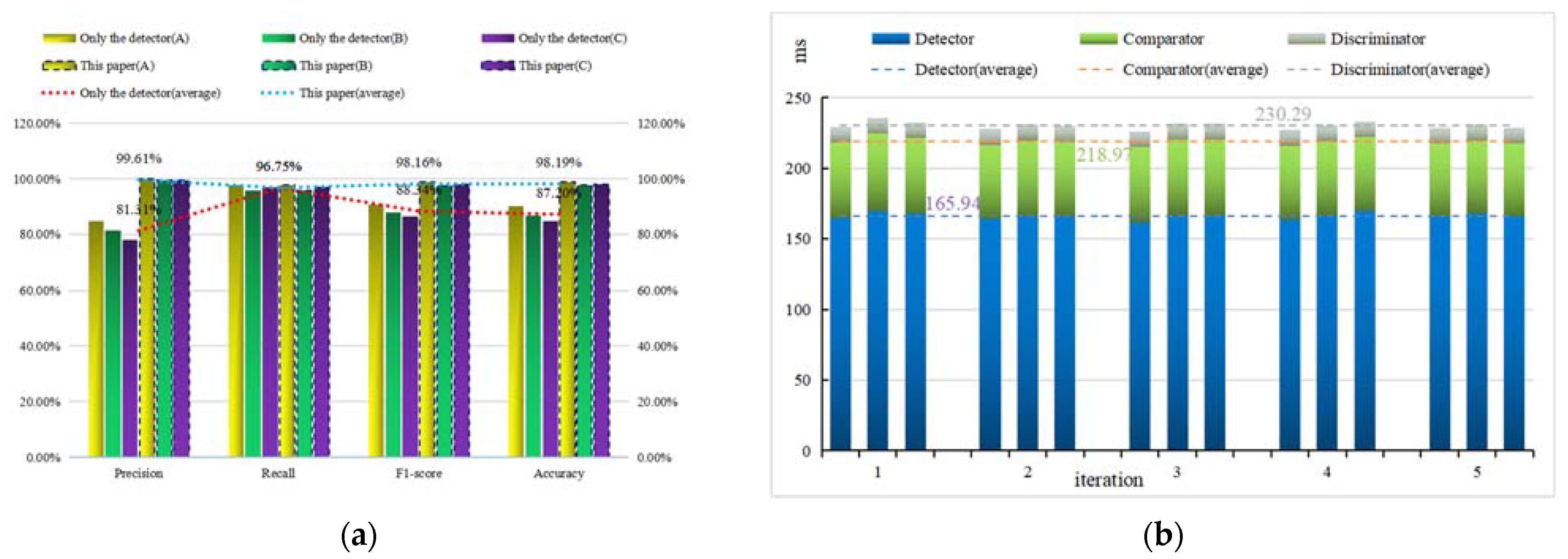
4. Results and Discussion
5. Conclusions
- A CNFA for surface defect detection combining a comparator, detector, and discriminator is proposed. Collect the non-defective image to construct the negative sample, retrieve the reference image with the help of the comparator; obtain the result rectangular frame of the detection image through the detector, and obtain the corresponding reference rectangular frame. Finally, the discriminator judges the true and false defects of the resulting rectangle to improve the detection accuracy;
- Based on the modified VGG16 network, the 1024-dimensional feature vector of the detection image and the negative sample set is extracted, and the Pearson correlation coefficient is used to measure the distance between each other, and the corresponding image with the smallest search distance is the reference image;
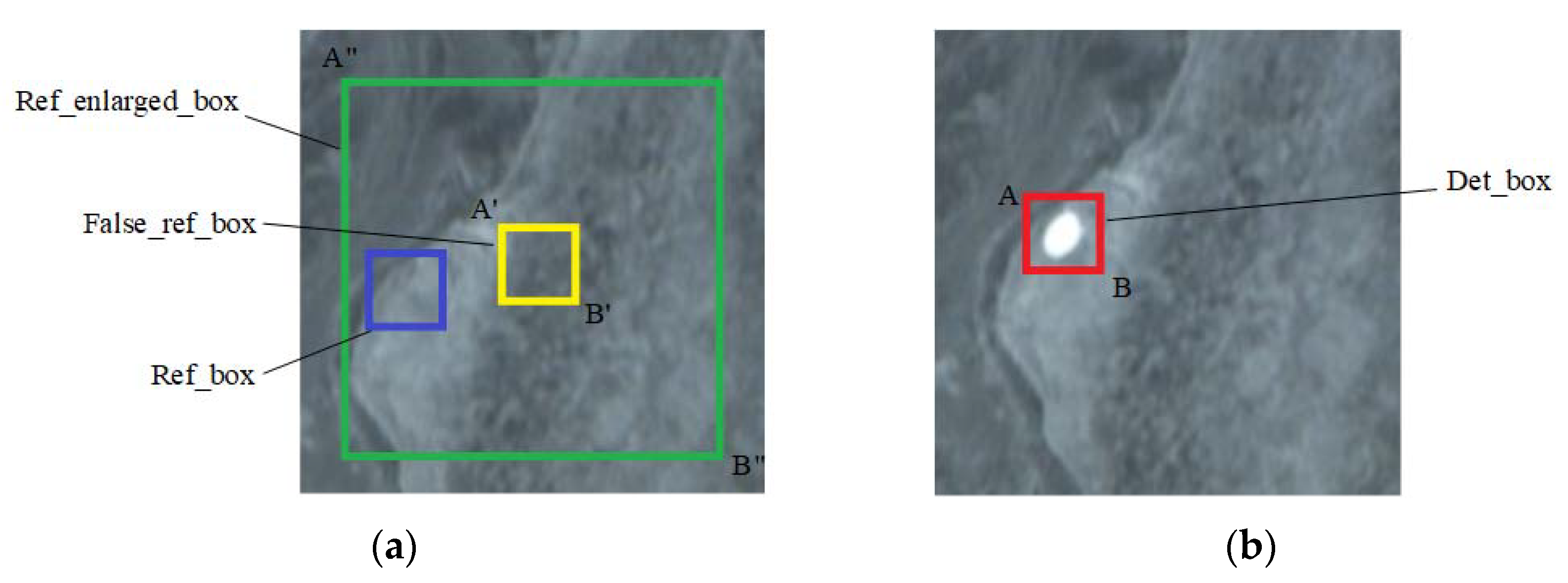
- The detector is composed of Resnet101 + FPN + Cascade R-CNN network structure. According to the coordinates of det_boxes obtained through the detector, the corresponding box on the reference image is magnified byβtimes. Then, the coordinate box of the maximum correlation coefficient is obtained by the correlation coefficient matching method, which is the ref_box;
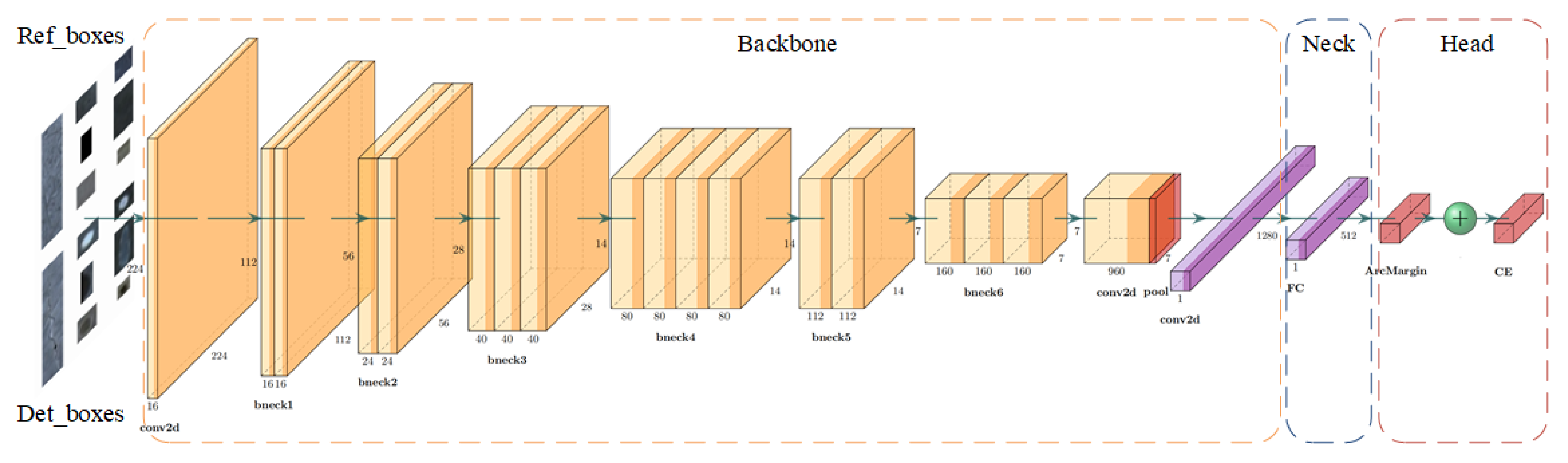
- The discriminator is composed of the modified MobileNetV3-Large as the backbone, combined with neck and head parts. The loss function based on the combination of Arc-margin and CE-Loss improves the network’s feature discrimination ability of defects and background textures. Then calculate the cosine distance of the feature vectors of det_boxes and ref_boxes; the smaller the result, the greater the texture probability, otherwise it is a defect;
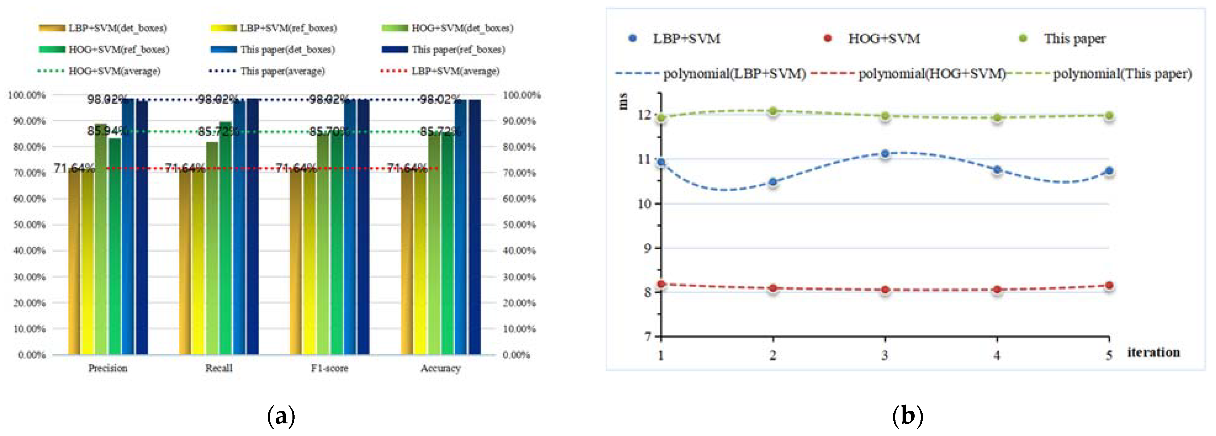
- After comparing with other methods on the verification set and test set, the accuracy and efficiency of our algorithm are proven. On the verification set, the accuracy of the discriminator reached 98.02%; on the test set, the average accuracy of the entire algorithm reached 98.19%, and the detection time of a single tile only increased by 64.35 ms.
Author Contributions
Funding
Institutional Review Board Statement
Informed Consent Statement
Data Availability Statement
Conflicts of Interest
References
- Mariyadi, B.; Fitriyani, N.; Sahroni, T.R. 2D Detection Model of Defect on the Surface of Ceramic Tile by an Artificial Neural Network. J. Phys. Conf. Ser. 2021, 1764, 012176. [Google Scholar] [CrossRef]
- Matić, T.; Aleksi, I.; Hocenski, Ž. CPU, GPU and FPGA Implementations of MALD: Ceramic Tile Surface Defects Detection Algorithm. Automatika 2014, 55, 9–21. [Google Scholar] [CrossRef] [Green Version]
- Zhao, Z.K. Review of non-destructive testing methods for defect detection of ceramics. Ceram. Int. 2021, 47, 4389–4397. [Google Scholar] [CrossRef]
- Sioma, A. Automated Control of Surface Defects on Ceramic Tiles Using 3D Image Analysis. Materials 2020, 13, 1250. [Google Scholar] [CrossRef] [PubMed] [Green Version]
- Li, D.; Niu, Z.; Peng, D. Magnetic Tile Surface Defect Detection Based on Texture Feature Clustering. J. Shanghai Jiaotong Univ. (Sci.) 2019, 24, 663–670. [Google Scholar] [CrossRef]
- Hanzaei, S.H.; Afshar, A.; Barazandeh, F. Automatic detection and classification of the ceramic tiles’ surface defects. Pattern Recognit. 2017, 66, 174–189. [Google Scholar] [CrossRef]
- Casagrande, L.; Macarini, L.A.B.; Bitencourt, D.; Fröhlich, A.A.; de Araujo, G.M. A new feature extraction process based on SFTA and DWT to enhance classification of ceramic tiles quality. Mach. Vis. Appl. 2020, 31, 1–15. [Google Scholar] [CrossRef]
- Zhang, H.; Peng, L.; Yu, S.; Qu, W. Detection of Surface Defects in Ceramic Tiles with Complex Texture. IEEE Access 2021, 9, 92788–92797. [Google Scholar] [CrossRef]
- Zorić, B.; Matić, T.; Hocenski, Ž. Classification of biscuit tiles for defect detection using Fourier transform features. ISA Trans. 2021. [Google Scholar] [CrossRef]
- Prasetio, M.D.; Rifai, M.H.; Xavierullah, R.Y. Design of Defect Classification on Clay Tiles using Support Vector Machine (SVM). In Proceedings of the 2020 6th International Conference on Interactive Digital Media (ICIDM), Bandung, Indonesia, 14–15 December 2020; pp. 1–6. [Google Scholar] [CrossRef]
- Zhang, J.; Zhang, H.Y.; Zhao, Y.G.; Sima, Z.W. Tile Defects Detection Based on Morphology and Wavelet Transformation. Comput. Simul. 2019, 36, 462–465. [Google Scholar]
- LI, J.H.; Quan, X.X.; Wang, Y.L. Research on Defect Detection Algorithm of Ceramic Tile Surface with Multi-feature Fusion. Comput. Eng. Appl. 2020, 56, 191–198. [Google Scholar]
- Liu, C.; Zhang, J.; Lin, J.P. Detection and Identification of Surface Defects of Magnetic Tile Based on Neural Network. Surf. Technol. 2019, 48, 330–339. [Google Scholar]
- Wang, K.; Li, Z. A new method to reduce the false detection rate of ceramic tile surface defects online inspection system. In Proceedings of the Tenth International Symposium on Ultrafast Phenomena and Terahertz Waves (ISUPTW 2021), Chengdu, China, 16–19 June 2021; Volume 11909, pp. 5–13. [Google Scholar] [CrossRef]
- Li, Z.H.; Chen, X.D.; Lian, T.Q. Surface Defect Detection of Ceramic Tile Based on Convolutional AutoEncoder Network. Mod. Comput. 2021, 27, 109–114. [Google Scholar]
- Junior, G.S.; Ferreira, J.; Millán-Arias, C.; Daniel, R.; Junior, A.C.; Fernandes, B.J. Ceramic cracks segmentation with deep learning. Appl. Sci. 2021, 11, 6017. [Google Scholar] [CrossRef]
- Huang, W.; Zhang, C.; Wu, X.; Shen, J.; Li, Y. The detection of defects in ceramic cell phone backplane with embedded system. Measurement 2021, 181, 109598. [Google Scholar] [CrossRef]
- Stephen, O.; Maduh, U.J.; Sain, M. A Machine Learning Method for Detection of Surface Defects on Ceramic Tiles Using Convolutional Neural Networks. Electronics 2022, 11, 55. [Google Scholar] [CrossRef]
- Bhatt, P.M.; Malhan, R.K.; Rajendran, P.; Shah, B.C.; Thakar, S.; Yoon, Y.J.; Gupta, S.K. Image-based surface defect detection using deep learning: A review. J. Comput. Inf. Sci. Eng. 2021, 21, 040801. [Google Scholar] [CrossRef]
- Yang, J.; Li, S.; Wang, Z.; Dong, H.; Wang, J.; Tang, S. Using deep learning to detect defects in manufacturing: A comprehensive survey and current challenges. Materials 2020, 13, 5755. [Google Scholar] [CrossRef]
- Hammad, I.; El-Sankary, K. Impact of approximate multipliers on VGG deep learning network. IEEE Access 2018, 6, 60438–60444. [Google Scholar] [CrossRef]
- Jebli, I.; Belouadha, F.Z.; Kabbaj, M.I.; Tilioua, A. Prediction of solar energy guided by pearson correlation using machine learning. Energy 2021, 224, 120109. [Google Scholar] [CrossRef]
- Karimi, M.H.; Asemani, D. Surface defect detection in tiling Industries using digital image processing methods: Analysis and evaluation. ISA Trans. 2014, 53, 834–844. [Google Scholar] [CrossRef] [PubMed]
- He, K.; Zhang, X.; Ren, S.; Sun, J. Deep residual learning for image recognition. In Proceedings of the IEEE Conference on Computer Vision and Pattern Recognition, Las Vegas, NV, USA, 27–30 June 2016; pp. 770–778. [Google Scholar] [CrossRef] [Green Version]
- He, K.; Gkioxari, G.; Dollár, P.; Girshick, R. Mask r-cnn. In Proceedings of the EEE International Conference on Computer Vision (ICCV), Venice, Italy, 22–29 October 2017; pp. 2961–2969. [Google Scholar] [CrossRef]
- Cai, Z.; Vasconcelos, N. Cascade r-cnn: Delving into high quality object detection. In Proceedings of the IEEE Conference on Computer Vision and Pattern Recognition, Salt Lake City, UT, USA, 18–22 June 2018; pp. 6154–6162. [Google Scholar] [CrossRef] [Green Version]
- Yu, C.C.; Sa, L.B.; Ma, X.Q. Few-shot parts surface defect detection based on the metric learning. Chin. J. Sci. Instrum. 2020, 41, 214–223. [Google Scholar]
- Howard, A.; Sandler, M.; Chu, G.; Chen, L.C.; Chen, B.; Tan, M.; Wang, W.; Zhu, Y.; Pang, R.; Vasudevan, V.; et al. Searching for mobilenetv3. In Proceedings of the IEEE/CVF International Conference on Computer Vision, Seoul, Korea, 27–28 October 2019; pp. 1314–1324. [Google Scholar] [CrossRef]
- Deng, J.; Guo, J.; Xue, N.; Zafeiriou, S. Arcface: Additive angular margin loss for deep face recognition. In Proceedings of the IEEE/CVF Conference on Computer Vision and Pattern Recognition, Long Beach, CA, USA, 15–20 June 2019; pp. 4690–4699. [Google Scholar] [CrossRef] [Green Version]


| No. | Type of Defects Detected | Type of Used Feature | Background Texture of CTs | Defects Discrimination | Evaluation Metrics |
|---|---|---|---|---|---|
| [1] | Corner or edge, glaze, pin-hole, cracks | GLCM | Simple textures | Without | Accuracy: 83% |
| [4] | Cracks | Morphological transformation | Without | Without | Not indicated |
| [5] | Cracks, pit and damage defects | Gabor energy spectra | Without | Without | Not indicated |
| [6] | Pin-holes, holes, cracks | Invariant rotation measure of local variance | Without | Without | Accuracy: 93.4% |
| [7] | Cracks, holes and spots | GLCM, HOG, DWT, SFTA | Without and monochromatic | Without | Accuracy: 99.01%, 93.2% |
| [8] | Spots, breakage, melt holes, wear scars, and cracks | Color spatial distribution variance | One texture; two textures, three textures | Color spot area weight features added as a discriminator | Accuracy: 98.4%, 96.2% and 91.21% respectively |
| [9] | Cracks and spots | Fourier transform | Black Random Stripes, brown light stripes | Without | F1-score: 92.36% and 88.66% |
| [10] | Cracks | LBP | without | Without | Accuracy: 87.5% |
| [11] | Cracks | Morphology and wavelet transform | without | Without | Not indicated |
| [12] | Cracks and spots | SIFT and color moments | Gray and colored textures | Without | Highest accuracy: 92.6% |
| [13] | Pits, notches, cracks, grinding | U-Net model | Without | Without | Accuracy: 94% |
| [14] | Cracks, dirt | Deep neural network | Complex textures | With a comparator | The average false detection rate: 5.8% |
| [15] | Cracks, holes | A lightweight convolutional auto-encoding network | Simple textures | Without | F1-score: 94.8% and 87.6% |
| [16] | Cracks | U-Net | Simple textures | Without | Precision: 99.9%; Recall: 78.7% |
| [17] | Cracks | YOLOv3-tiny | Simple textures | Without | Accuracy: 89.9% |
| Category Item | Non-Defective Images | Defective Images | Reference Boxes | Defective Boxes |
|---|---|---|---|---|
| Discriminator training set | 6000 | 6000 | 14,852 | 14,852 |
| Discriminator validation set | 322 | 322 | 781 | 781 |
| Test set | 524 | 524 |
| Type of Defects | Corner Crack | Edge Crack | Collapsed Surface | White Border | Pinhole |
|---|---|---|---|---|---|
| legend |  |  |  |   |  |
| Type of defects | Crack | Pull line | Soiling | Glaze bubble | Lack of glaze |
| legend |  |  |  |  |  |
| Type of defects | Delamination | Scratch | dripping ink | Cave | |
| legend |  |  |  |  |
| Item SN Number | A | B | C | |||
|---|---|---|---|---|---|---|
| Texture type | Light color | Medium gray | Dark gray | |||
| legend |  | 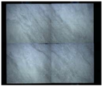 | 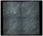 | |||
| Category | Defective | Non-defective | Defective | Non-defective | Defective | Non-defective |
| Number | 170 | 170 | 167 | 167 | 187 | 187 |
| True Results | Prediction Results | |
|---|---|---|
| Positive | Negative | |
| Positive | True Positive (TP) | False Negative (FN) |
| Negative | False Positive (FP) | True Negative (TN) |
| SN | Method | Items | True Number | TP | FN | FP | TN |
|---|---|---|---|---|---|---|---|
| 1 | LBP + SVM | Defective boxes | 781 | 557 | 224 | 219 | 562 |
| Reference boxes | 781 | 562 | 219 | 224 | 557 | ||
| 2 | HOG + SVM | Defective boxes | 781 | 639 | 142 | 81 | 700 |
| Reference boxes | 781 | 700 | 81 | 142 | 639 | ||
| 3 | This paper | Defective boxes | 781 | 761 | 20 | 11 | 770 |
| Reference boxes | 781 | 770 | 11 | 20 | 761 |
| SN | Method | SN | Defective | Non-Defective | TP | FN | FP | TN |
|---|---|---|---|---|---|---|---|---|
| 1 | Independent detector | A | 170 | 170 | 166 | 4 | 30 | 140 |
| B | 167 | 167 | 160 | 7 | 37 | 130 | ||
| C | 187 | 187 | 181 | 6 | 51 | 136 | ||
| 2 | This paper | A | 170 | 170 | 166 | 4 | 0 | 170 |
| B | 167 | 167 | 160 | 7 | 1 | 166 | ||
| C | 187 | 187 | 181 | 6 | 1 | 186 |
| No. | Number of Defects Detected | Background Texture of CTs | Defect Discrimination | Evaluation Index |
|---|---|---|---|---|
| [1] | 5 | Simple textures | Without | Accuracy: 83% |
| [6] | 3 | Without | Without | Accuracy: 93.4% |
| [7] | 3 | Without and monochromatic | Without | Accuracy: 99.01%, texture: 93.2% |
| [8] | 6 | One texture, two textures, three textures | With | Accuracy: 98.4%, 96.2% and 91.21% |
| [9] | 2 | Black Random Stripes, brown light stripes | Without | F1-score: 92.36% and 88.66% |
| [10] | 1 | Without | Without | Accuracy: 87.5% |
| [12] | 2 | Gray and colored textures | Without | Highest accuracy: 92.6% |
| [13] | 4 | Without | Without | Accuracy: 94% |
| [14] | 2 | Complex textures | With | Accuracy: 94.2% |
| [15] | 2 | Simple textures | Without | F1-score: 94.8% and 87.6% |
| [16] | 1 | Simple textures | Without | Precision: 99.9%; Recall:78.7%, F1-score:88% |
| [17] | 1 | Simple textures | Without | Accuracy: 89.9% |
| [18] | 1 | Simple textures | With | Accuracy: 99.43% |
| The CNFA | 14 | Complex textures | With | The average accuracy: 98.19%, The average F1-score: 98.16% |
Publisher’s Note: MDPI stays neutral with regard to jurisdictional claims in published maps and institutional affiliations. |
© 2022 by the authors. Licensee MDPI, Basel, Switzerland. This article is an open access article distributed under the terms and conditions of the Creative Commons Attribution (CC BY) license (https://creativecommons.org/licenses/by/4.0/).
Share and Cite
Wang, K.; Li, Z.; Wang, X. Concatenated Network Fusion Algorithm (CNFA) Based on Deep Learning: Improving the Detection Accuracy of Surface Defects for Ceramic Tile. Appl. Sci. 2022, 12, 1249. https://doi.org/10.3390/app12031249
Wang K, Li Z, Wang X. Concatenated Network Fusion Algorithm (CNFA) Based on Deep Learning: Improving the Detection Accuracy of Surface Defects for Ceramic Tile. Applied Sciences. 2022; 12(3):1249. https://doi.org/10.3390/app12031249
Chicago/Turabian StyleWang, Kan, Zeren Li, and Xu Wang. 2022. "Concatenated Network Fusion Algorithm (CNFA) Based on Deep Learning: Improving the Detection Accuracy of Surface Defects for Ceramic Tile" Applied Sciences 12, no. 3: 1249. https://doi.org/10.3390/app12031249
APA StyleWang, K., Li, Z., & Wang, X. (2022). Concatenated Network Fusion Algorithm (CNFA) Based on Deep Learning: Improving the Detection Accuracy of Surface Defects for Ceramic Tile. Applied Sciences, 12(3), 1249. https://doi.org/10.3390/app12031249