A FE-Based Macro-Element for the Assessment of Masonry Structures: Linear Static, Vibration, and Non-Linear Cyclic Analyses

Featured Application

The macro–element formulated in the study can be implemented in any FE–based software for the static (quasi–) and dynamic analysis of masonry structures. It assures an attractive computational cost and accuracy level with respect to standard continuous FE models.

Abstract

A Finite Element (FE) based macro–element is described for the mechanical response of masonry structures within different ranges of analysis. The macro–element is composed of discrete rigid quadrilateral FE plates whose adjoining interfaces are connected through FE trusses. It allows representing both elasticity and strength orthotropy, full material nonlinearity and damage through a scalar–based model. The possibility of coupling with a so–called FE² (multi–scale) strategy is also addressed. Validation of the macro–element is conducted within linear static, vibration, and cyclic (nonlinear) problems, in which both static and dynamic ranges are explored. Results are compared with those retrieved from traditional FE continuous models. Advantages are highlighted, as well as its robustness to cope with convergence issues and suitability to be applied within more general and larger–scale scenarios, such as the analysis of anisotropic materials subjected to static and dynamic loading. Formal details are given for its reproducibility by academics and practitioners—eventually within other FE platforms—as the improved running times may be of utmost importance in dynamic problems or highly nonlinear (material) quasi–static analysis.

1. Introduction

Masonry is a phenomenological complex material due to the elastic and strength anisotropies, its well–marked nonlinear response in tension, compression, and shear regimes [1], and due to the potential damage–induced anisotropy. Experimentation reveals the difficulty of predicting the mechanical response of masonry [2]. Such difficulties are consistent with the substantial number of works developed during the last decades aiming the assessment of masonry structures. These can be grouped within simplified or advanced approaches [3,4,5].

In the scope of structural analysis for masonry buildings, the prevailing design rules or analytical approaches are the most useful for practitioners, despite the possible unrealistic or conservative outcomes [6]. Other simplified procedures, such as the story–mechanism [7] and the equivalent frame–based models [8,9,10], can be found; in hand with the keen development and improvement of macro–elements that constitute the geometric features of masonry structures (such as walls, piers, and spandrels) [11,12,13,14,15]. The reduced degrees–of–freedom make these suitable for the study of large–scale and regular structures. Yet, these suffer from a macro–element discretisation bias, demand proper strength criteria for each macro–element type, and hardly consider out–of–plane failure modes. More suitable and yet conceptually simple procedures, such as the rigid–body approaches [16,17] or the kinematic methods [18,19,20,21,22], are useful to supply closed–form solutions under dynamic excitations, although are still overly complex for walls subjected to two–way bending.

In this context, the need for more general methods encouraged the development of advanced numerical strategies, such as the Discrete Element Method (DEM) and the Finite Element Method (FEM) [23]. DEM presents several advantages since allows one to represent masonry as a discontinuous media, in which masonry units are considered as the ensemble of distinct bodies connected by contact surfaces (joints). Since the first DEM model proposed by Cundall and Hart [24], and the discontinuous deformation analysis (DDA) introduced by Shi and Goodman [25], several studies have been introduced with masonry as a specific target [26]. DEM is widely applied to simple blocky structures [5]; for instance, in the analysis of arches to assess the collapse load [27], the static and dynamic analysis of masonry walls [2,28,29,30,31,32,33], and the rocking motion of stone blocks [34]. Software dedicated to this formulation exists, see [35,36]. Although DEM unfolds inherent advantages, the modelling of three–dimensional complex or large structures, with a high number of block elements, can make the computational time unacceptable. Besides, simplifications concerning the mesh discretisation may compromise the accuracy and, therefore, may be taken carefully. As stated by Lemos [26], the accuracy for the out–of–plane study of masonry is quite dependent on the number of contact points in the thickness direction. Regardless of the latter, DEM is still rarely applied for three–dimensional structures within a dynamic analysis.

To what concerns FEM, its overall use deserves wide acceptance from the scientific community [4]. FE–based models have a broad range of applications because they can be employed either in simple or complex geometric structural configurations, and either within static or dynamic problems. These are typically classified according to the followed modelling strategy, namely: (i) direct numerical simulation or micro–modelling approach; (ii) macro–modelling approach; and (iii) multi–scale computational approach. In the direct numerical simulation, both masonry components (units and mortar joints) are explicitly represented. Both in– and out–of–plane orthotropic nonlinear behaviour can be reproduced, but long processing times are expected, hence being only recommended for limited size structural problems [26,37,38,39,40,41,42,43,44,45]. Macro–modelling approaches tend to be adopted in the study of large–scale structures [46,47]. Masonry is modelled as an equivalent homogeneous media and damage is smeared out over a mesh region (the so–called localisation band), which goes against how it is generally found in masonries, i.e., concentrated or distributed following clear failure patterns [5,19]. Multi–scale FE approaches (usually two–scale or FE²) are in–between the latter modelling schemes. Different scales of analysis are directly employed to describe the mechanical behaviour of the media, often provided by a homogenisation–based procedure [45,48,49,50,51,52] at the foregoing scale. Although very promising, the use of full–continuum FE strategies at both scales is computationally prohibitive when material nonlinearity is accounted [53]. In–depth (formulation) assumptions that allow decreasing such cost with acceptable accuracy are certainly of interest, as recently proposed in [54,55,56].

The strong literature background makes FE models a popular built–in method for structural analysis. Furthermore, the increase of computational processing power—noticing the upcoming quantum computing—may allow its scalability to larger and larger scales. Nonetheless, the computational cost in the dynamic range is still prohibitive and both numerical instabilities and convergence issues are contentious in the quasi–static range, as when modelling laminar structures composed of materials with highly nonlinear behaviour. Similarly, assumptions that offer the possibility of using simplified (still accurate) FE models are important as they allow lessening the required complexity of problems. From a logical extent, the inherent advantages will be fully explored if the coarser scale of analysis is adopted, i.e., the so–called macro–modelling. The study of structures with larger dimensions may allow the representation of the material using a broader domain that, in some cases, can be enough to catch the phenomenological features of interest. The underlying assumption is that the interaction between brick units and mortar joints can be neglected for the global structural behaviour, hence valid if the difference between macro– and meso–scales is sufficiently large. It is usually referred that a ratio (characteristic lengths) between 10 to 100 is questionable for periodic masonry [57]. The heterogenous masonry media is then replaced by an equivalent homogeneous material, in which the constitutive relation is taken as an average one. This requires complex phenomenological formulations to reproduce material orthotropy and to follow the damage onset and propagation. In this endeavour, continuous FE–based macroscopic strategies are the most spread in the literature, in which two frameworks have arisen to catch failure: using discontinuities for the explicit modelling of cracks through the so–called cohesive zones [58,59,60], or in a continuous way using classical or enriched (with crack–tracking algorithms) smeared–cracking models [61,62,63,64,65]. Although damage representation may lack detail at the crack level, it is known that these numerical models are still adequate for the study of concrete, concrete–like, and masonry materials at a structural level. In such a scope, the riddle lies in the definition of the most suitable modelling approach, by considering its dimensions, study purpose, and that a trade–off between accuracy and practicability is evaluated (also in terms of computational time). If the latter is respected, i.e., the characteristic length at the macro–level holds, then macro–models are suitable. Therefore, simplified FE macro–modelling approaches can be followed, such as those based on limit analysis [66,67,68,69,70] or on discontinuous or discrete FE–models [70,71,72,73,74,75,76,77].

In this regard, the study tries to give a formal description of an improved macro–element that originally stems from [78]. It allows retrieving the mechanical response of masonry structures adopting a macro–modelling approach and within attractive computational costs. The main goal is to foster its reproducibility, aiming at the use by academics and practitioners when performing seismic assessment (or related) studies. First, the kinematics of the macro–element is presented for both in–plane and out–of–plane modes, together with essential steps to scale and regularise the material constitutive relationships. Then, formal validation of the macro–element is performed within linear static, vibration, and cyclic (uni– and bi–directional) problems. At last, computational features that are considered relevant are stated.

2. Macroscopic Unit–Cell

2.1. Theoretical Scope

The macro–element has a theoretical background on the works of Kawai [79,80,81] and was implemented in the ABAQUS software. The strategy is especially suited for the study of planar elements, i.e., for a three–dimensional body, ${\mathsf{\Omega }}_M\subseteq {\Re }^3$, with one dimension much smaller than the other two. Such an assumption is also postulated when studying a given structure with a plate or flat shell FE’s. Therefore, the modelling using the macro–element tries to describe the structure using the mid–surface of the body, ${\mathsf{\Omega }}_M$. Given the cartesian space and for the undeformed configuration, it is assumed that the thickness t of the structure develops in the z–direction $\left(z=\left[-t/2,+t/2\right]\right)$ and that the two planar coordinates are defined through global x and y coordinates (see Figure 1). Such an assumption is important to recall bearing the integration with a multi–scale framework, as it should be linked with the Cartesian system adopted at a meso/micro–scale. A uniformisation between the allowable macro–deformation modes and the respective meso–scale ones is convenient when material orthotropy exists.

The macroscopic unit–cell is composed of the assemblage of discrete quadrilateral rigid plate elements connected through a set of rigid and deformable FE trusses in its interfaces. Rigid plates are modelled as four linear quadrilateral elements within a finite–membrane strain formulation (S4 element in ABAQUS). Full integration is adopted to prevent hourglass modes. The rigid linear elements are defined as three–dimensional Timoshenko FE beams (B31 in ABAQUS). In this scope, the deformation and damage of the structure are restricted to three–dimensional two–node FE trusses (T3D2 in ABAQUS). These are comparable with spring elements since they have just one DOF and are directly integrated. Their stiffness matrix is defined only by axial stiffness terms, given by $diag\left(\frac{EA}{L},\frac{EA}{L}\right)$, in which E is the Young’s modulus, A is its cross–section area and L is its axial length. The macro–deformation is thus governed by the trusses, in which in– and out–of–plane failure modes are considered within a decoupled approach.

The FE trusses incorporate the material information, in which both orthotropy and full softening behaviour can be provided by defining the properties of the different interface sides. Regarding the out–of–plane (OOP) behaviour, the macroscopic cell is composed of a set of four flexural and torsional trusses. The flexural trusses are placed at the mid–centre of each interface and the torsional trusses are placed at each node of the squared rigid plate. Mid–span hinges on interfaces allow the fixing of the axis of rotation for torsion movements without compromising the deformed shape. Regarding the in–plane (IP) modes, trusses have been assumed for axial and shear behaviours. For the former, a total of three axial trusses are placed per–interface (two in the edges and one in the centre), and for the latter, a total of two shear trusses (defining the shear for each half–length of the interface) have been placed per interface.

Inertial forces can be either modelled via a direct lumped or consistent mass matrix strategy. The former requires the computation of the representative mass for each rigid plate and its introduction through nodal mass elements on each rigid plate node. The latter allows it to be more straightforward, as the mass of the system is embodied by the quadrilateral rigid plates using an equivalent material density. By following a linear displacement interpolation assumption, one achieves a consistent mass matrix. Still, a comparison between both strategies will be given in Section 3.1.2. The computation of the system density ${\rho }_{system}$ is given as ${\rho }_{real}.t/t_{eq}$, t being the real thickness of the structural element, ${\rho }_{real}$ the real density of the material, and $t_{eq}$ the thickness attributed to the rigid plates (defined as 10 mm).

At last, it may be noticed that since the macro–element has been implemented using an FE software, a stiffness matrix $\left[{\rm K}\right]\in {\Re }^{n\times n}$ (n is the number of DOFs) has to be assembled for a given structure to compute the displacements vector $\left[u\right]\in {\Re }^n$, with respect to the action of a vector of external forces $\left[f\right]\in {\Re }^n$ through the weak–form $\left[{\rm K}\right]\left[u\right]=\left[f\right]$. In this scope, the plates are enforced to be rigid (for both the axial and bending cases) by defining a high Young’s modulus given by ${10}^{10}$ MPa (and a thickness of 10 mm). Likewise, the rigid linear elements are defined to have a high Young’s modulus given by ${10}^{12}$ MPa (and a section area of 0.1 mm²). The definition of the latter values may be questionable, as flexible elements of the system become connected with disproportionately stiffer ones and can turn $\left[{\rm K}\right]$ ill–conditioned [82]. Nonetheless, authors report that such values have been properly defined as having in mind such issues and that, for the stiffness values typically associated with concrete–like materials, these can be used with no further concern.

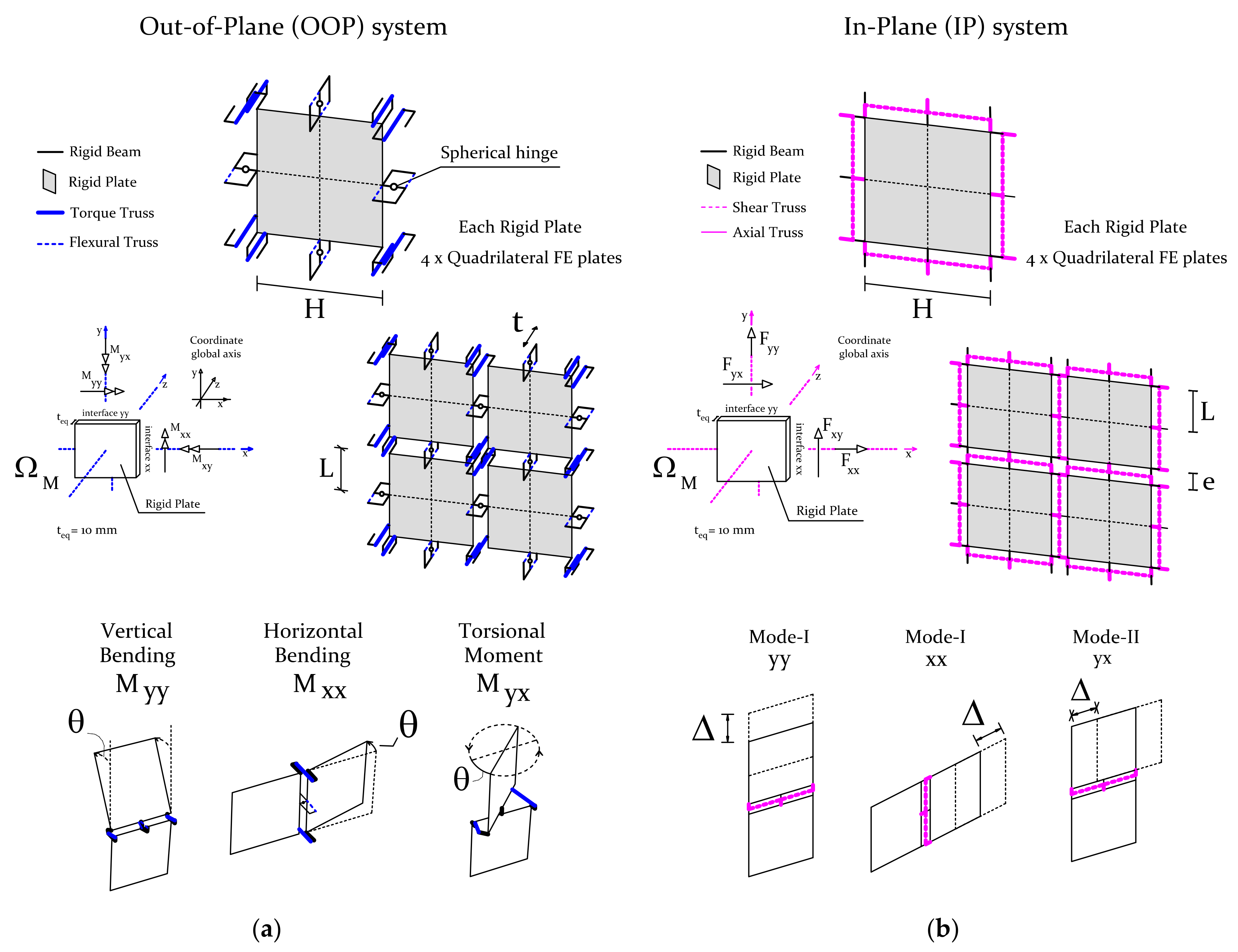
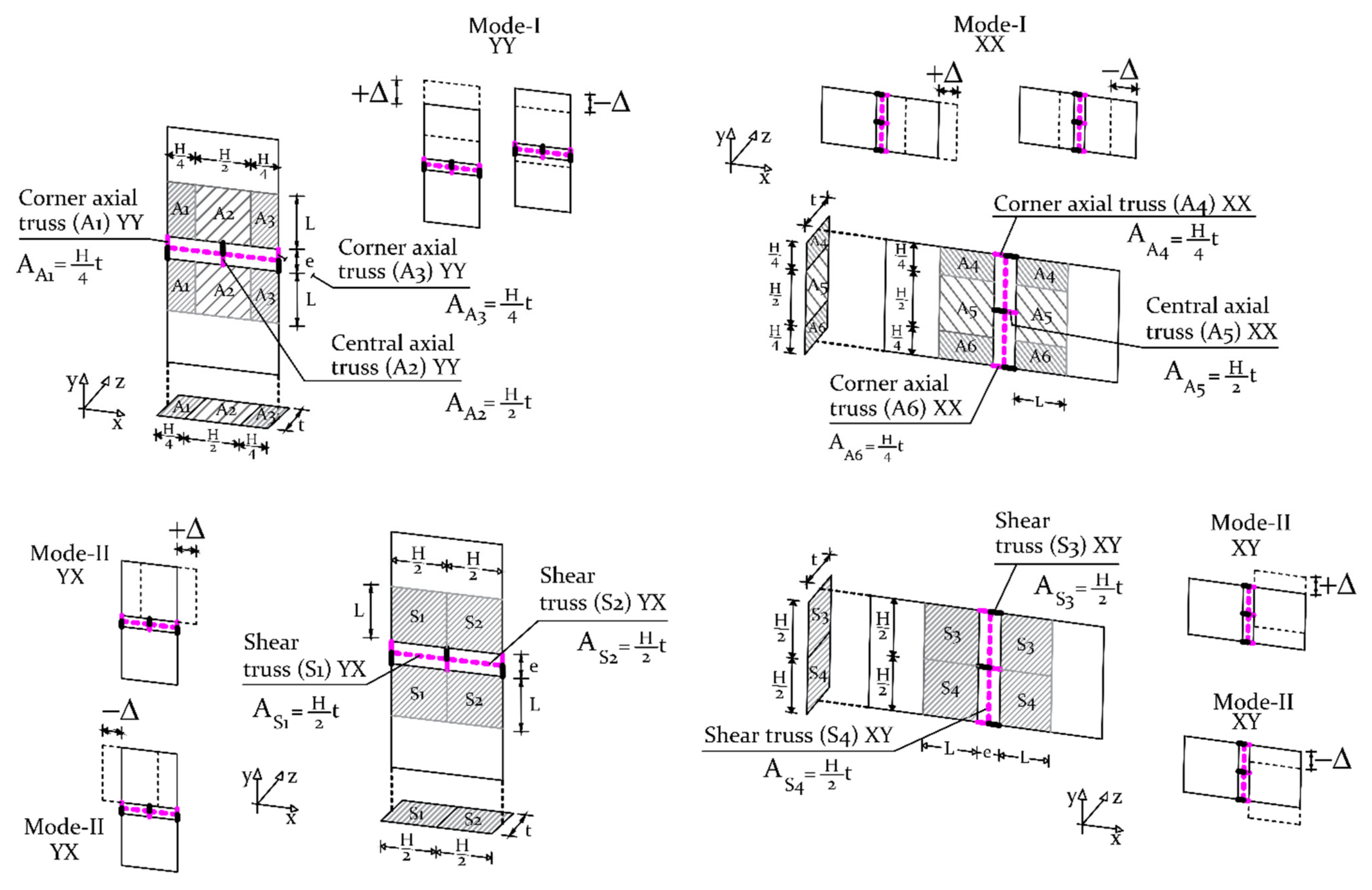
2.2. In–Plane Kinematics

The variational principle of energy conservation and the principle of virtual displacement were followed to achieve the discrete macro–element elastic stiffnesses. Figure 2 presents the two directions of the in–plane system, i.e., the x– and y–directions, with both the tributary areas of each in–plane FE truss and the associated deformation modes (kinematics).

Let us consider that ${\overline{E}}_{ii}$ is the elastic modulus of the equivalent homogeneous material $(\overline{}$ is the average operator as it is generally defined to represent a composite or intrinsically homogeneous material), i is the corresponding axis x or y, ${\overline{G}}_{xy}$ the shear modulus of the media, V the volume of the region under study, and $\Delta$ a displacement increment under the studied direction. For the in–plane case, the total strain energy density is generically given by Equation (1):

$$U=\frac{1}{2}{{\displaystyle \int }}_V{\left\{\mathsf{\Sigma }\right\}}^T\left\{E\right\}\cdot dV$$

(1)

where ${\left\{\mathsf{\Sigma }\right\}}^T=\left\{\begin{array}{ccc}{\mathsf{\Sigma }}_{xx}& {\mathsf{\Sigma }}_{yy}& {\mathsf{\Sigma }}_{xy}\end{array}\right\}$ and $\left\{E\right\}=\left\{\begin{array}{ccc}{E}_{xx}& E_{yy}& E_{xy}\end{array}\right\}$ are the stress and strain quantities of the media constitutive relationship, respectively, ideally obtained experimentally or via a homogenisation procedure. For the mode–I, the calibrated elastic stiffness of each in–plane truss is derived by imposing that the stored strain energy in volume V of both the discrete $U_{discrete}^{mode-I}$ and the continuum homogenised media $U_{continuum}^{mode-I}$ are equal.

$$U_{continuum}^{mode-I}=\frac{\sigma \epsilon }{2}V=\frac{{\overline{E}}_{ii}{\epsilon }^2}{2}V=\frac{H.t.{\overline{E}}_{ii}}{2}\frac{{\Delta }^2}{2L+e}$$

(2)

$$U{U}_{discrete}^{mode-I}=V\frac{\sigma \epsilon }{2}=\frac{H.t.E_{ii}^{in-plane axial truss}}{2}\frac{2{\Delta }^2}{e}$$

(3)

If both energies are equated, the Young’s modulus of the in–plane axial trusses of a macro–unit cell for each plane direction (if orthotropy is considered) are derived and reads as:

$$E_{xx}^{in-plane axial truss}=\frac{{\overline{E}}_{xx}e}{4L+2e}$$

(4)

$$E_{yy}^{in-plane axial truss}=\frac{{\overline{E}}_{yy}e}{2\left(H+e\right)}$$

(5)

The same methodology is followed for the mode–II trusses, namely the in–plane shear trusses. The stored strain energies of the continuum and discrete model are:

$$U_{continuum}^{mode-I}=\frac{H.t.{\overline{G}}_{xy}}{4}\frac{{\Delta }^2}{2L+e}$$

(6)

$$U_{discrete}^{mode-II}=\frac{e.t.E_{xy}^{in-plane shear truss}{\Delta }^2}{H}$$

(7)

Consequently, the Young’s modulus of the in–plane shear trusses are given by:

$$E_{xy}^{in-plane shear truss}=\frac{{\overline{G}}_{xy}{H}^2}{4e\left(2L+e\right)}$$

(8)

For more details regarding the IP formulation, the reader is referred to [83,84].

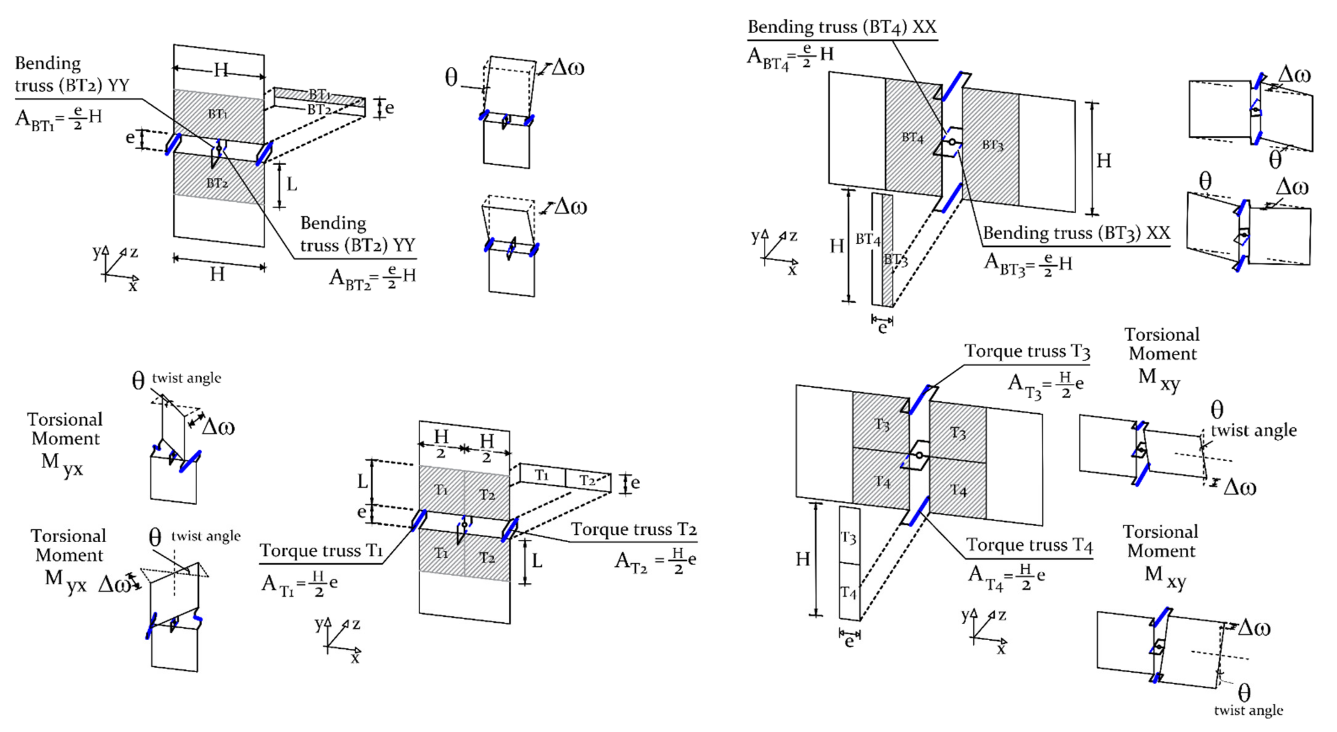
2.3. Out–of–Plane Kinematics

The variational principles of energy conservation and virtual displacements were followed to compute the elastic stiffnesses of the out–of–plane FE trusses; as provided for the in–plane case. Figure 3 depicts the out–of–plane basic cell of the macro–element. The geometrical parameters and the respective tributary areas for flexural and torsional FE trusses are given. Additionally, the kinematics of each allowable deformation mode is associated with a moment quantity defined in the input, or by integrating the in–plane stress–strain curves in the thickness direction.

Equivalence between the bending energies of the discrete $\left(U_{discrete}^{bending}\right)$ macro–element and a continuum $(U_{continuum}^{bending})$ plate media is postulated to retrieve the latter expressions. In such regard, the $U_{continuum}^{bending}$ of a continuous FE plate subjected to bending is derived from Equation (9):

$$U=\frac{1}{2}{{\displaystyle \int }}_l^{}\frac{M^2}{EI}dl$$

(9)

and given by:

$$U_{continuum}^{bending}=\frac{1}{2}\left({\overline{E}}_{ii}I\right){\chi }^2\left(H+e\right)=\frac{{\overline{E}}_{ii}H{t}^3}{24\left(1-{\nu }^2\right)}\left(H+e\right)$$

(10)

The stored strain bending energy of the discrete system is derived through an ad–hoc formulation. Bearing that the strain of the axial out–of–plane truss–beams is $\epsilon =\raisebox{1ex}{$\theta e$}\!\left/ \!\raisebox{-1ex}{$t$}\right.$ and $\theta =\chi \left(H+e\right)$, $U_{discrete}^{bending}$ is given as:

$$U_{discrete}^{bending}=\frac{1}{2}M\theta =\frac{1}{2}\frac{E_{ii}^{bending truss}{A}_{t}e}{t}{\theta }^2$$

(11)

By equating $U_{continuum}^{bending}=U_{discrete}^{bending}$ the correct Young’s modulus of the OOP flexural trusses is calculated according to Equation (12):

$$E_{ii}^{bending truss}=\frac{{\overline{E}}_{ii}{t}^{4}H}{24e\left(1-{\nu }^2\right)\left(H+e\right)e{A}_t}$$

(12)

For torsion, the same procedure is followed. Briefly, the stored strain torsional moment energies of the discrete and continuum homogeneous media are given by Equations (13) and (14), as follows:

$$U_{continuum}^{torsional}=\frac{\overline{G}H{t}^3{\theta }^2}{24\left(2L+e\right)}$$

(13)

$$U_{discrete}^{torsional}=\frac{E^{torsional truss}e{H}^3{\theta }^2}{16t}$$

(14)

in which $\overline{G}$ is the homogenised shear modulus given directly by the slope of the in–plane shear constitutive law. Thus, by respecting the energy equivalence between the systems, the correct Young’s modulus of the torsional trusses is defined through Equation (15).

$$E_{}^{torsional truss}=\frac{2\overline{G}{t}^4}{3H^{2}e\left(2L+e\right)}$$

(15)

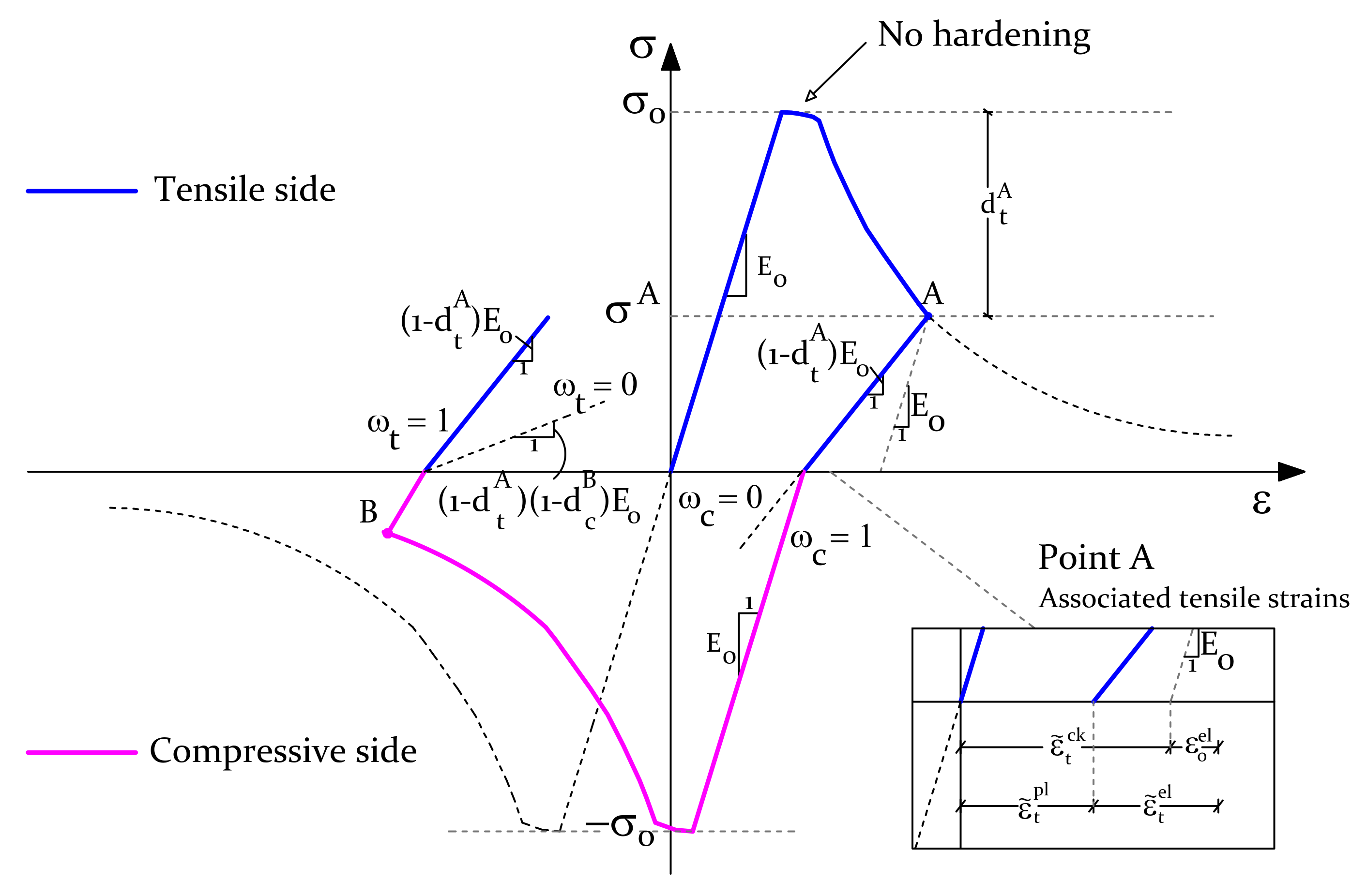
2.4. Material Constitutive Law and Damage Model

A proper macro–constitutive law must be assigned to the elements that govern both the deformation and inelastic response of the interfaces, i.e., the FE trusses. The constitutive model tries to mimic the material information provided—potentially via at a foregoing scale through a homogenisation procedure—and, therefore, should be capable to allocate the mechanical information and effectively represent the elastic and inelastic behaviours.

Although several plasticity models can be adopted in ABAQUS, the concrete damage plasticity (hereafter, CDP) model has been selected given the better representation of the inelastic laws. The model combines stress–based plasticity with strain–based scalar damage. It can reproduce several macroscopic properties for tension and compression regimes, such as (i) different yield strengths; (ii) different stiffness degradation values; (iii) different recovery effect terms; and (iv) rate sensitivity, which can increase the peak strength value depending on the response strain rate. Moreover, it does consider the latter in the presence of interfaces that are dynamic and/or cyclic loading, and is integrated using the backward Euler method (see Figure 4). A general overview of the main features of CDP for the rate–independent model is presented next, being the reader referred to, e.g., [85,86] for further details.

Effective stresses govern the plastic part of these models [87] and the stress–strain relationship is ruled, as referred, by an isotropic damage scalar affecting the elastic stiffness of the material. According to Equation (16) the nominal stress tensor $\sigma$ reads:

$$\sigma =\left(1-d\right)E_0^{el}\left(\epsilon -{\epsilon }^{pl}\right)=E:\left(\epsilon -{\epsilon }^{pl}\right)$$

(16)

where $E_0^{el}$ is the initial elastic stiffness of the material; d is the damage parameter, which defines the stiffness degradation (0 for an undamaged and 1 for a fully damaged material), and is designated as d_t and d_c for tension and compression regimes, respectively; $\epsilon$ is the total strain tensor; ${\epsilon }^{pl}$ is the plastic strain tensor; and E is the initial elastic stiffness of the material affected by the damage parameters (the degraded initial stiffness given by E $=\left(1-d\right)E_0^{el}$).

Regarding the softening variables, Equation (17) describes the law $h$ that expresses their evolution, in which ${\dot{\epsilon }}^{pl}$ is the plastic multiplier (assuming a non–associated potential flow), and ${\tilde{\epsilon }}^{pl}$ and $\overline{\sigma }$ are the equivalent plastic strain tensor and the effective stress tensor, respectively.

$${\dot{\tilde{\epsilon }}}^{pl}=h\left(\overline{\sigma },{\tilde{\epsilon }}^{pl}\right){\dot{\epsilon }}^{pl}$$

(17)

The CDP model uses a yield function based on the works in which a hardening variable $K_c$ controls the meridian shape of the yield function. A $K_c=2/3$ is assumed, leading to an approximation of the Mohr–Coulomb criterion. Three other dimensionless parameters need to be defined, i.e., the dilation angle,$\mathsf{\Psi }$, the eccentricity, $\mathrm{e}$, and the viscosity parameter. The dilation angle $\mathsf{\Psi }$ is measured in the p–q plane and gives the inclination angle of the failure surface in respect to the hydrostatic axis; from a physical standpoint, it represents the internal friction angle of the material. Here, a value of 30 degrees has been defined. The eccentricity parameter $\mathrm{e}$ modifies the flow potential rule, being a straight line if $\mathrm{e}=0$ and a hyperbola if $\mathrm{e}=0.1$. The default value, i.e., $\mathrm{e}=0.1$, has been assumed. The viscosity parameter is introduced to enhance the results convergence in the presence of material and/or geometrical nonlinearities, through a viscoplastic regularisation by Duvaut and Lions [88]. This parameter should be treated with care as it can misrepresent the obtained results. For the present macro–element, the default value of 0 (zero) has been adopted, even though it has been noticed that within a quasi–static pushover analysis a value of $1\times {10}^{-4}$ can decrease the computational cost without apparently affecting the results.

Since truss beams define the material behaviour of the interfaces, the system will undergo only uniaxial loading conditions and, therefore, the plastic strain rates in tension, ${\dot{\epsilon }}_t^{pl}$, and compression, ${\dot{\epsilon }}_c^{pl}$, are a function of the uniaxial plastic strain rate, ${\dot{\epsilon }}_{11}^{pl}$, and read as:

$${\dot{\epsilon }}_t^{pl}={\dot{\epsilon }}_{11}^{pl}{\mathrm{and}\dot{\epsilon }}_c^{pl}=-{\dot{\epsilon }}_{11}^{pl}$$

(18)

Likewise, even if the CDP has been extended for the general multiaxial conditions, the uniaxial character of the system may also be adopted for the cyclic loading analysis, which simplifies, to a great extent, its follow–up validation. In such cases, the recovery of the elastic stiffness when the sign of the imposed load changes is an important aspect to consider. The so–called ‘unilateral effect’ holds both in tensile and compressive sides of the cycle, in which, for uniaxial conditions, the damage parameter variable d is given as:

$$\left(1-d\right)=\left(1-s_t{d}_c\right)\left(1-s_c{d}_t\right){,s}_t\ge {0,s}_c\le 1$$

(19)

Here, $s_t$ and $s_c$ are functions of the stress state which represents the referred stiffness recovery with the related stress reversals and are defined as:

$$\left\{\begin{array}{c}\begin{array}{c}{s}_{t }=1-{\omega }_t{r}^{*}\left({\overline{\sigma }}_{11}\right)\\ \end{array}\\ s_c = 1-{\omega }_c\left(1-r^{*}\left({\overline{\sigma }}_{11}\right)\right)\end{array}\right.$$

(20)

Here, ${\omega }_t$ and ${\omega }_c$ are weight factors and assumed as input material parameters for the CDP model and limited by $0\le {\omega }_t\le 1$ and $0\le {\omega }_c\le 1$, and $r^{*}\left({\overline{\sigma }}_{11}\right)=1$ if ${\overline{\sigma }}_{11}>0$ or $r^{*}\left({\overline{\sigma }}_{11}\right)=0$ if ${\overline{\sigma }}_{11}<0$. In concrete–like materials, the effect is more marked when the material is in a compression regime $({\sigma }_{11}<0)$, because tensile cracks tend to close [86]. Nevertheless, the aim here is to fully reproduce the homogenised behaviour in both regimes and so the Bauschinger effect is not reproduced. Therefore, the tensile and compressive elastic stiffnesses have a full recovery effect, which is the same as defining ${\omega }_t= 1$ and ${\omega }_c=1$.

To fulfil the input requirements of the CDP model in ABAQUS, information regarding the post–failure behaviour may be introduced for each element that features material nonlinearity, i.e., the truss beams, in terms of stress and inelastic strain ${\tilde{\epsilon }}_{}^{ck}$ values. The latter must be obtained for each point of the post–peak homogenised curve by Equation (21):

$${\tilde{\epsilon }}_{}^{ck}=\epsilon -{\epsilon }_o^{el}$$

(21)

in which ${\epsilon }_o^{el}$ is the elastic strain corresponding to the undamaged material and $\epsilon$ is the total axial strain of the multi–linear stress envelope. If the damage parameters, $d$, are introduced, the plasticity model is thus coupled with a damage description and is suitable for the cyclic behaviour description of the material. The plastic strain values, ${\epsilon }^{pl}$, are calculated, for each point of the curve, as:

$${\epsilon }^{pl}={\epsilon }^{cr}-\frac{d}{\left(1-d\right)}\frac{{\sigma }^P}{E_0^{el}}$$

(22)

Since the permanent plastic strain can be just positive or null, the latter can constitute a good checkpoint to foresee if the damage parameters have been properly computed. Lastly, it is important to recall that to increase the robustness of the problem, and as given in Figure 4, multi–linear curves (e.g., with 5–nodes) are defined. Furthermore, a small plateau near the peak strength of the curve is recommended, to circumvent an abrupt stiffness loss, avoid potential convergence, and run–time problems. The adequacy of such approximation will be discussed in Section 3.

2.5. Material Information and Required Processing Steps

The material input for the macro–element interfaces (FE trusses) needs to be given in terms of stress–strain $(\mathsf{\Sigma }-\mathsf{E})$ and, through thickness integration, converted to moment–curvature $(\mathrm{M}-\mathsf{\chi })$ curves when out–of–plane behaviour is of interest. This information is employed at the macro–element after two processing steps, aiming to achieve a correct material characterisation, i.e., the so–called scaling and regularisation steps. These appear to be critical to assure that the macro–input is independent of the refinement (size) adopted for the macro–element.

Such transition steps are conducted after the preparation of the computational model, because it is dependent on the size of the used discrete mesh, particularly, on the values of H, e, L, and t. Furthermore, squared rigid elements are assumed, hence only two different are possible for the interfaces: 0 and 90 degrees. The material orthotropy is reproduced at a structural level because the approach offers the possibility to reproduce different input stress–strain relationships according to the trusses plane. For the in–plane behaviour, the stress quantities are directly derived from the input curves. For the out–of–plane system, the macroscopic homogenised moment values are adapted to follow representative stress values for the bending and torsional trusses through Equations (23) and (24):

$${\sigma }_{bending truss}=\frac{M}{(e.A_{BTruss})}$$

(23)

$${\sigma }_{tosional truss}=\frac{M}{(H.A_{TTruss})}$$

(24)

Here, M is the bending moment per unit of interface length; H is the size of each square rigid element or plate; t is the thickness of the wall; $A_{BTruss}$ is the bending truss area; $A_{TTruss}$ is the torque truss area; and $e$ is the gap between the rigid plates, which ideally should be zero but in practice is assumed small enough to be able to place trusses between the elements.

After the earlier stage, the stress–strain curves are regularised by defining the elastic stiffness and fracture energy terms. The regularisation step is necessary to properly find the elastic stiffness of each truss beam and to guarantee the input independence from the macro–mesh and, thus, its objectivity in the nonlinear range. One raises the similarities with the regularisation concept firstly addressed by Bažant and Oh [89] in which the fracture energy terms are regularised by a crack bandwidth parameter, $l_{crack}$; albeit, more sophisticated approaches exist, such as those who convey on non–local methods [90,91].

By assuring the elastic energy equivalence between the discrete model and a continuum homogeneous plate, it is possible to derive the so–called regularisation factor, ${\mathrm{f}}_r$—this scaling operator affects the strain values of the curves that serve as an input. Within a decoupled behaviour, the latter is performed separately for the in–plane, axial (mode–I and mode–IV) and shear (mode–II) deformations, and out–of–plane modes, i.e., both flexural and twisting movements. In this way four different ${\mathrm{f}}_r$ operators are found, which allow the holding of the energy equivalence assumption.

Briefly, let us consider, for instance, that $\tilde{\mathsf{E}}=\left[\begin{array}{cc}{\epsilon }_1& {\epsilon }_2\end{array}\cdots \begin{array}{cc}{\epsilon }_{n-1}& {\epsilon }_n\end{array}\right]$ and $\tilde{\mathsf{\Sigma }}=\left[\begin{array}{cc}{\sigma }_1& {\sigma }_2\end{array}\cdots \begin{array}{cc}{\sigma }_{n-1}& {\sigma }_n\end{array}\right]$ are the n–dimensional sets which define, respectively, the stress–strain input curves being regularised (n is the number of points of the curve). The correct elastic stiffness value, obtained through the energy equivalence demonstration, is computed for the point of the curve which has one–third of the peak stress value, designated as point p. The regularisation factor is given as $f_r={\sigma }_p/({\epsilon }_p{E}_{corrected})$, in which $E_{corrected}$ is the corrected Young’s modulus obtained for each truss type (see Section 2.2 and Section 2.3). This procedure is followed, and four regularisation factors are computed. By correcting the strain values of the curves, both the elastic stiffness and fracture energy terms are regularised.

3. Macro–Element Application

The mechanical validation of the macro–element is addressed next, with a clear focus on the study of the out–of–plane behaviour of masonry. Since the seminal works by Irons et al. [92,93,94], conducting patch tests has become a regular step when presenting finite elements, see [95,96,97,98,99] for a review. Zienkiewicz and Taylor [100] stated that, in plate problems, the ‘importance of the patch test in both the design and testing of the elements is paramount and this should never be omitted’.

Patch tests may be a trivial formality for standard finite elements because of the shape function’s continuity requirements, but its usefulness as a debugging step for code implementation is accepted. In this sense, some tests of comprehensiveness are employed over the macroscopic unit–cell element aiming to assess the reliability and convergence of the solution in elastic and inelastic problems for static and dynamic ranges.

3.1. Linear Range

Performance tests were conducted to evaluate the ability of the model in (i) elasticity problems, and (ii) in vibration analysis through the eigenmodes frequencies and deformed shapes.

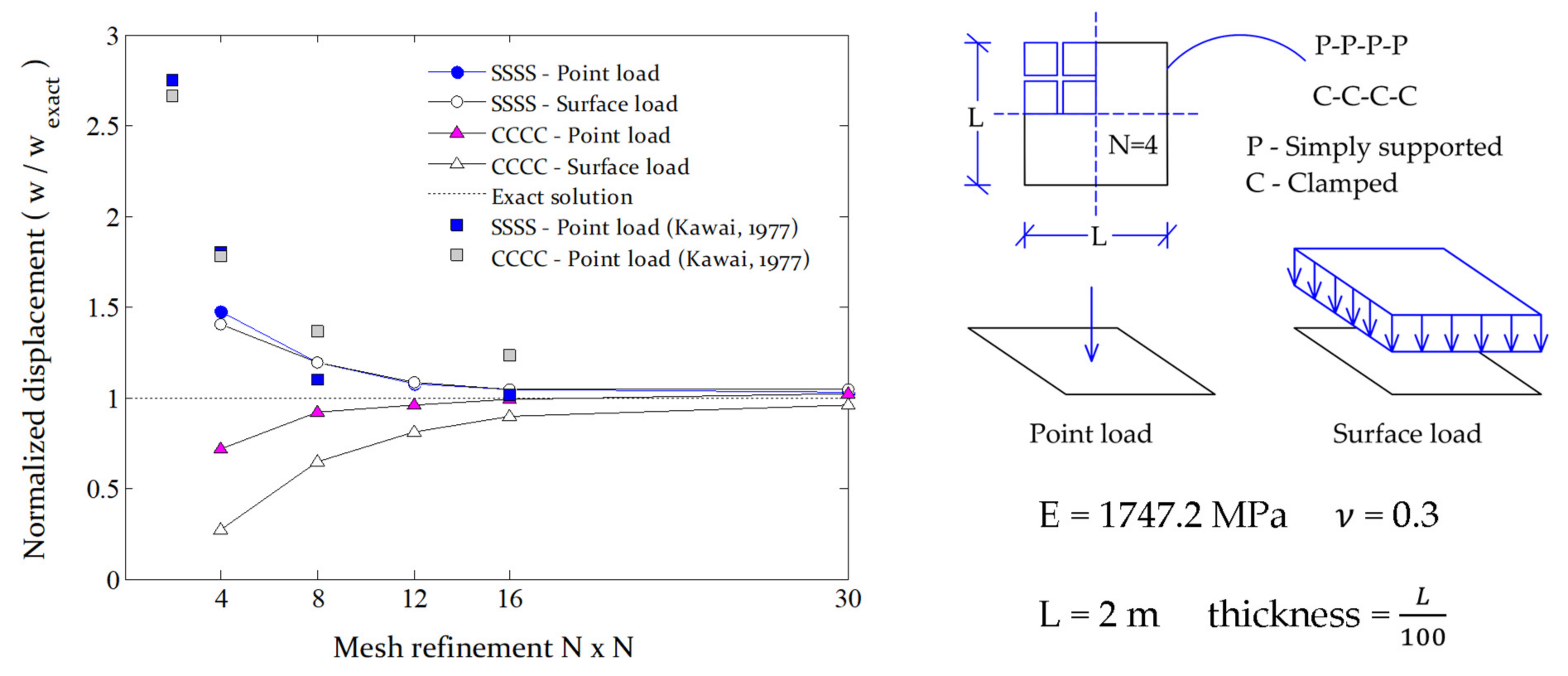
3.1.1. Elasticity Problems

The conducted test addresses a squared plate subjected to different loading cases and with two possible boundary conditions. The squared plate benchmark has a side length, L, and belongs to the set of patch tests proposed by Rao and Shrinivasa [99]. Aiming to especially serve as a reference test for plate bending elements, a thickness equal to $L/100$ is assumed, that approximates well thin–plate solutions. Two squared plates, one with pinned (SSSS) and the other with clamped supports (CCCC) at its edges, are subjected to a point and a surface (normal) load.

The convergence of the discrete macro–model has been assessed by comparing the maximum elastic displacement, $w$, obtained with the exact solution, $w_{exact}$, for different mesh refinement levels, N. The maximum deflection obtained at the centre of the plate is normalised with the exact theoretical solution and presented in Figure 5. Although the discrete element behaves better in the presence of simply supported edges, which is to be expected given the lower gradients of curvature, the load type seems to have a further extent on the solution accuracy. The model can better reproduce the point load behaviour due to its localised effect, which goes in favour with the data from the Rigid–Body–Spring model (RBSM) developed by Kawai [79]. Globally, a refinement of $N=15$ ($H=L/15$) is a proper choice allowing estimations within 10% of a maximum deflection error. Hence, a higher refinement is recommended for clamped edges ($N=L/16$) than simply supported edges ($N=L/12$).

The plate benchmark test is inexpensive to carry out and a time–cost analysis has been disregarded. The value of the errors found are admissible and in agreement with typical simplified mixed–FE strategies, as the RBSM by Kawai [79] and the Hermann–Hellan constant–stress–triangular elements [101]. Besides the simplification adopted for the decoupled flexural–torsional behaviour, it may be emphasised that the deviations found, especially when clamped supported edges exist, stem from the macro–element assumptions. Quadrilateral elements are adopted which restrains the model adaptability and deformability near cornered regions. Therefore, a mesh bias occurs near the supports that explains the stiffer responses found for the clamped edges cases, i.e., no deformation exists within a distance from the border given by the mesh size H. This also supports the fact that the response is different than classical continuous FE–based models since it gives lower bound estimations of the displacement (for different mesh refinements).

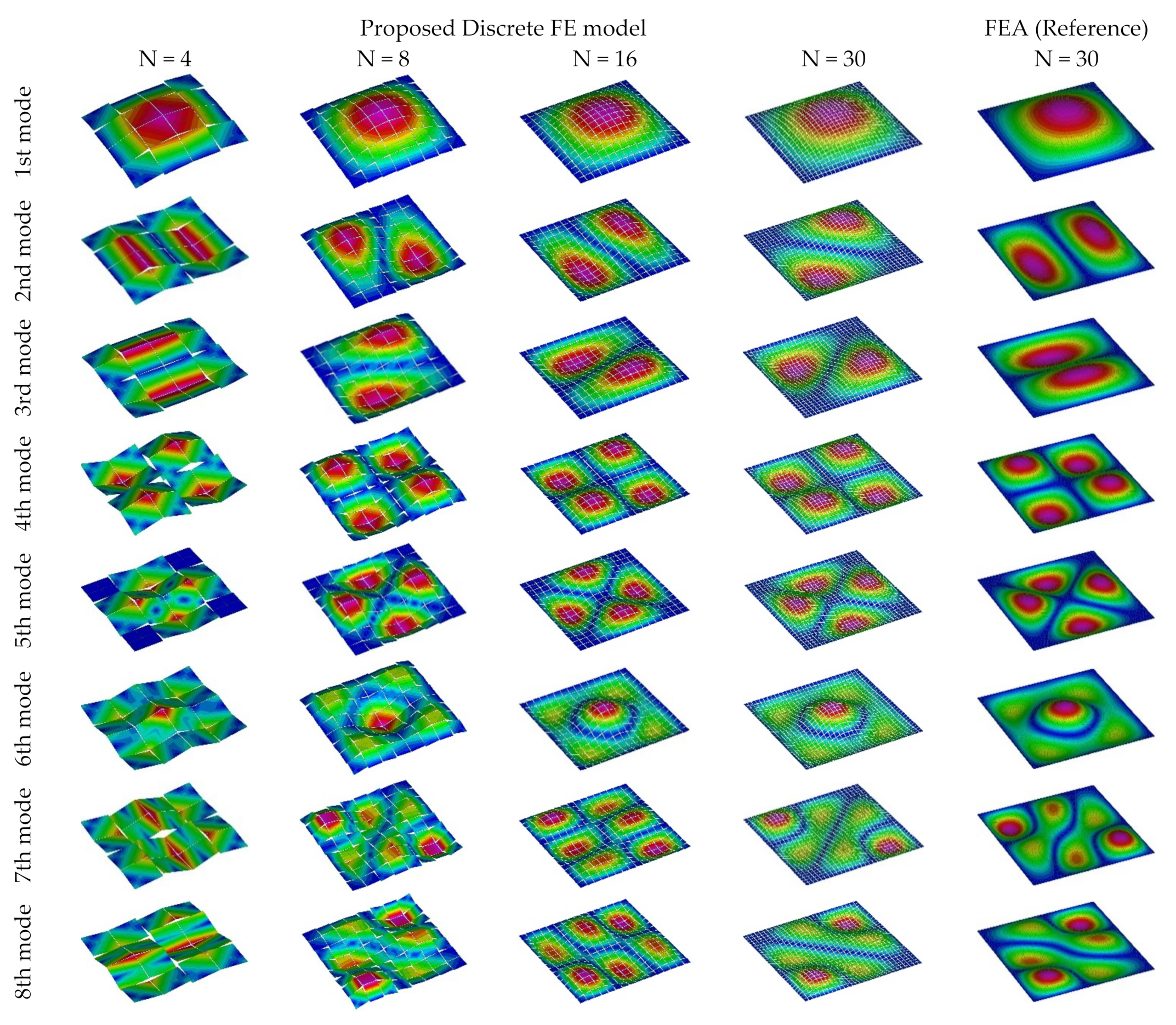
3.1.2. Vibration Analysis

Free vibration analysis is conducted in a simply supported squared plate. The plate is isotropic and shows uniform thickness, t, and mass density values, $\rho$. The free harmonic vibration of a thin plate is governed by the following differential equation:

$$D{\nabla }^{4}w\left(x,y\right)-{\omega }^2\rho tw\left(x,y\right)=0$$

(25)

Here, $w\left(x,y\right)$ is a given mode in the cartesian space, ${\nabla }^4$ is the biharmonic differential operator in Cartesian coordinates, i.e., ${\partial }^2/\partial x^2+{\partial }^2/\partial y^2$, and D is the bending stiffness given as $E{t}^3/12/\left(1-{\upsilon }^2\right)$. For the present example, a squared plate simply supported at its four edges, the solution of the vibration mode shapes has been formulated by Navier [102]:

$$w\left(x,y\right)=A_{mn}\sin \left(\frac{m\pi x}{a}\right)\sin \left(\frac{n\pi y}{a}\right) , \left(m,n=1,2,\dots \right)$$

(26)

in which, $A_{mn}$ is the amplitude of vibration (which are the unknown coefficients), m is the number of half–waves in the x–direction, n is the number of half–waves in the y–direction, and $a$ is equal to the length, L, of the squared plate side. By replacing Equation (26) in the differential equation, one obtains the exact solution for the vibration of frequencies in terms of the parameters m and n:

$$\omega =\sqrt{\frac{D}{\rho t}}\left[{\left(\frac{m\pi }{L}\right)}^2+{\left(\frac{n\pi }{L}\right)}^2\right]$$

(27)

By adopting different values for the integer parameters m and n, the theoretical and exact frequencies of the first eight modes have been found. For the discrete model, since it relies on an FE–based strategy, the natural frequencies and mode shapes are obtained through the following matrix form equation:

$$\left(\left[K\right]-{\omega }^2\left[M\right]\right)\left\{w\right\}=0$$

(28)

Here, [K] and [M] are the global stiffness and mass matrices. The mass of the discrete system is carried by the rigid plate elements by providing a representative density value, ${\rho }_{system}$. Uniform mass distribution is assumed to assemble the mass matrix either through a lumped or consistent strategy. The former admits that the mass of the rigid plate is lumped in its nodes, this allowing to obtain a diagonal mass matrix. In the consistent strategy, mass is distributed in the rigid plates following a linear interpolation rule, as when computing the local stiffness matrix, and both translational and rotational inertias are accounted. Towards a convergence study, four mesh refinements have been considered:$N=4,N=8,N=16\mathrm{and}N=30$. A thickness value of L/10 and a gap spacing between the discrete cells of $e=20\mathrm{mm}$ have been admitted. Furthermore, the analysis is complemented with the results from a standard continuum FE model (with a mapped mesh, element size of $L/30$ and with a consistent mass matrix) designated as FEA. Results gathered in

Table 1. Convergence study: normalised natural frequencies $\left(\omega /{\omega }_{exact}\right)$ found for the proposed macro–model and a standard continuous Finite Element Analysis (FEA).

Mode	Macro–Element (Lumped Mass Approach)				Macro–Element (Consistent Mass Approach)				FEA N = 30	Exact (rad/s)	m	n
	N = 4	N = 8	N = 16	N = 30	N = 4	N = 8	N = 16	N = 30
1	1.276	1.094	1.026	1.025	1.244	1.088	1.064	1.024	1.000	19.739	1	1
2	1.382	1.085	1.037	1.037	1.302	1.069	1.064	1.034	1.000	49.348	1	2
3	1.382	1.085	1.037	1.037	1.294	1.069	1.064	1.034	1.000	49.348	2	1
4	1.499	1.129	1.036	1.028	1.371	1.103	1.073	1.031	1.001	78.957	2	2
5	1.405	1.088	1.047	1.045	1.276	1.053	1.063	1.039	1.000	98.696	1	3
6	1.475	1.084	1.046	1.045	1.218	1.049	1.061	1.039	1.000	98.696	3	1
7	1.569	1.143	1.045	1.038	1.356	1.099	1.075	1.036	1.001	128.30	3	2
8	1.569	1.143	1.045	1.038	1.355	1.099	1.075	1.036	1.001	128.30	2	3

are given as normalised angular frequencies (with the exact solution).

According to the h–refinement dependency verified in the elasticity problems considered before, a higher mesh refinement lead to lower errors. Yet, a mesh size of L/16 provides solutions with an error lower than 5% (lumped approach), which seems to constitute a sufficient refinement choice for larger case studies. A consistent mass matrix strategy yields more accurate eigenfrequency contents than the lumped one; that is especially clear for coarser meshes in which significant differences have been found (higher than 20%). On the other hand, the modal deformed shapes depicted in Figure 6 indicate that all the discretisation fit the FEA results up to the first four modes.

After that, coarser meshes are unable to catch higher modal responses, due to the implicit mechanical arrangement of the quadrilateral rigid elements. Nonetheless, the higher refinement ($L/30$) reproduces well all the modal displacements. At last, it may be pointed out that the choice between the best approach to distribute the mass matrix is arguable because the accuracy depends on the mesh refinement. Still, a consistent strategy is adopted hereafter.

3.2. Non–Linear Range

The main purpose of this section is to briefly assess if the nonlinear homogenised curve that serves as input for the constitutive material model (CDP) is properly attributed. This is accomplished by attesting if the CDP adopted for the macro–interfaces leads to the expected static and hysteretic responses. An ad–hoc simple case study is used for both purposes, namely a vertical masonry wall simply supported in its bottom and top edges and subjected to a centrally prescribed displacement, as depicted in Figure 7.

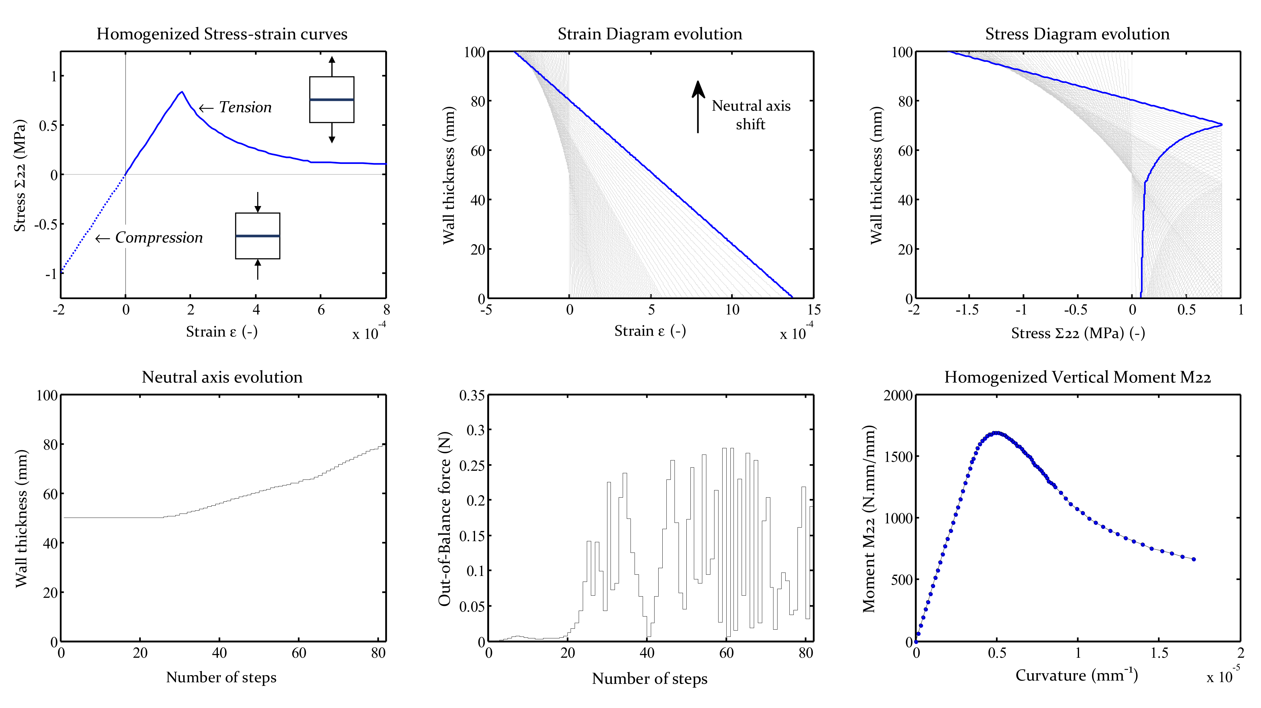
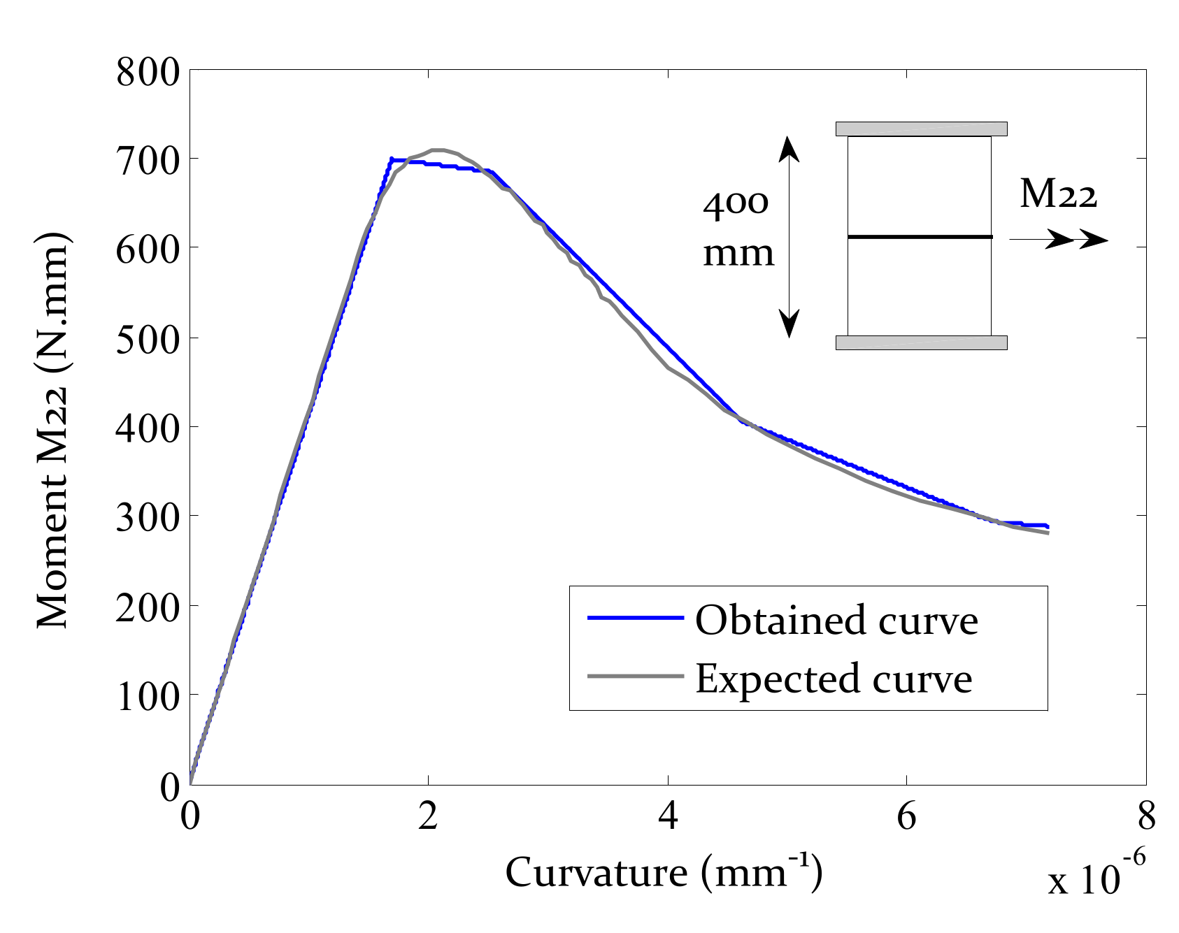
3.2.1. Quasi–Static (Monotonic) Nonlinear Curve

The first conceptual verification is performed through a quasi–static analysis. An out–of–plane displacement is applied at the centre of the masonry wall. The assumed stress–strain in–plane curves (${\mathsf{\Sigma }}_{yy}-{\mathsf{E}}_{yy}$ curves) are given in Figure 8. Specifically, a linear behaviour was assumed in compression, and a strength value of 0.80 MPa followed by exponential softening was assumed in tension. The corresponding vertical bending moment M₂₂ (designated as the principal stress couple, equivalent to M_yy) is obtained through–the–thickness integration of the wall using a Kirchhoff–plate theory, as given in Figure 8.

Following the required transitions steps addressed in Section 2.5, the calibrated and regularised $\sigma -\epsilon$ curves required for the vertical flexural truss beams have been identified and given in

Table 2. Input stress–strain ($\mathsf{\sigma }-\mathsf{\epsilon }$ ) curves for the FE trusses in the FE software (CDP model in ABAQUS).

Cracking Strain (–)	Stress (MPa)	Damage Scalar D (–)
0.00	9.61	0.00
5.06 × 10−5	9.41	0.20
2.11 × 10−4	5.57	0.42
3.49 × 10−4	4.03	0.58
6.09 × 10−4	3.36	0.65

. The quasi–static analysis allowed us to reach the wall’s structural response, whose capacity curve, in terms of bending moment–curvature, is represented in Figure 9 and compared with the expected one (M₂₂ homogenised curved for an $L=400$ mm). Results show that the strategy is well implemented and that adopting a simplified 6–node curve is adequate since the stored bending energy difference is, between the obtained and the theoretical curves, lower than 1%.

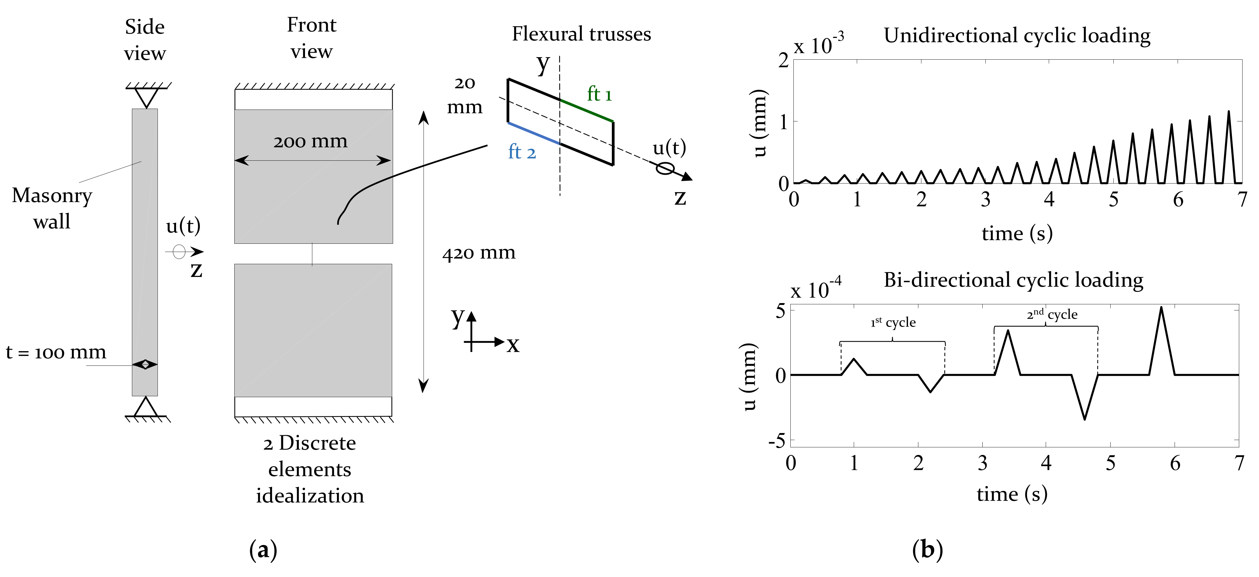
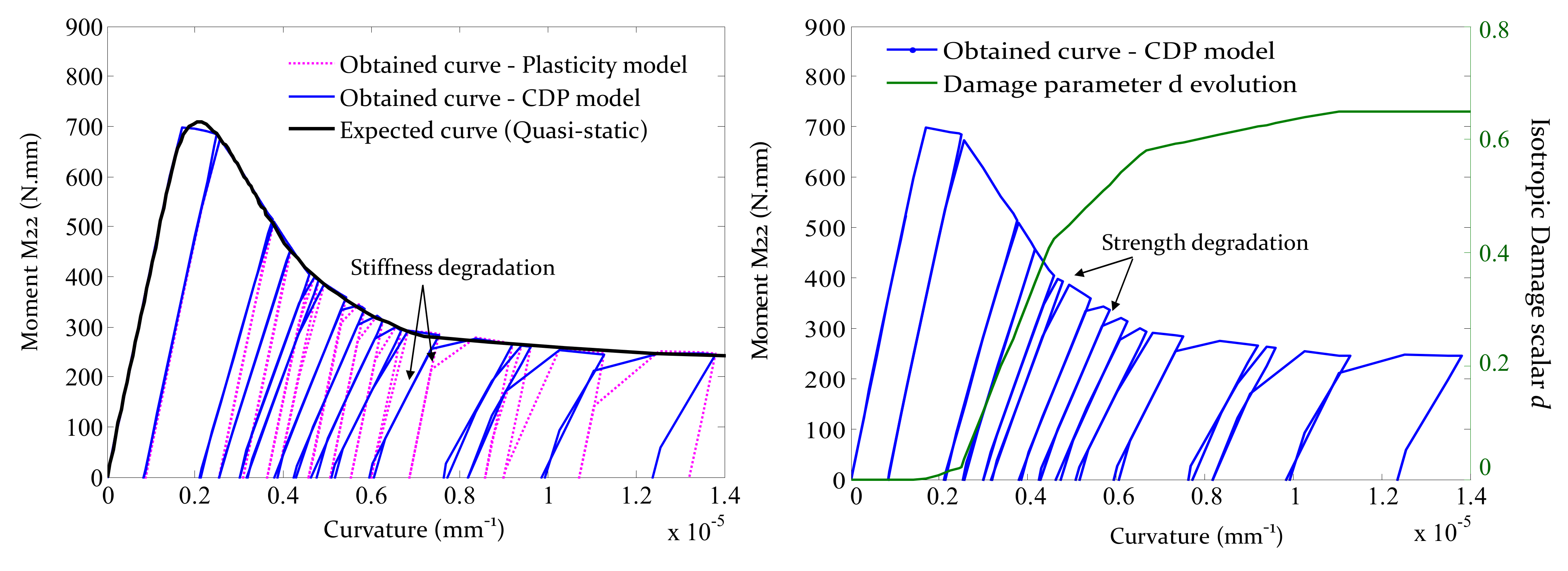
3.2.2. Uni–Directional Cyclic Loading

In classical plasticity theory, three key features are of utmost importance: the yield criterion, the flow rule, and the hardening/softening rule [85]. As referred, a Mohr–Coulomb yield failure envelope and a non–associated flow rule have been assumed. For the hardening rule, the model depends on the definition of cracking strains associated with given effective stresses. It is the purpose of the uni–directional cyclic test to verify if the latter is well reproduced for a cyclic type of loading. Towards the latter, the same case study of Figure 7 has been used. The process of strength deterioration is itself the pure representation of the softening rule evolution [85]. Figure 10 shows that the obtained skeleton curve using the CDP model fits the expected quasi–static curve.

Furthermore, a damage model is coupled with the plasticity one. The softening rule is interpreted through an isotropic damage variable, d, which is, by itself, a function of the equivalent plastic strains and, therefore, its value never decreases. Stiffness degradation of the material after cracking should be accounted. Figure 10 shows a comparison between the present CDP model and a pure plasticity model with an absence of stiffness degradation. On one hand, both phenomenological representations allow to achieve permanent material plastic deformations, but these are higher if a total plasticity model with initial unloading stiffness is adopted (known to be too conservative). On the other hand, the appearance of plastic strains is a manifestation of inelastic behaviour and, as Figure 10 proves, its evolution follows the expected path (see Table 2) reaching a constant value after the ultimate strain threshold limit, correspondent to a cracking strain of 6.09 × 10⁻⁴, in which the residual strength is defined and thus damage remains constant.

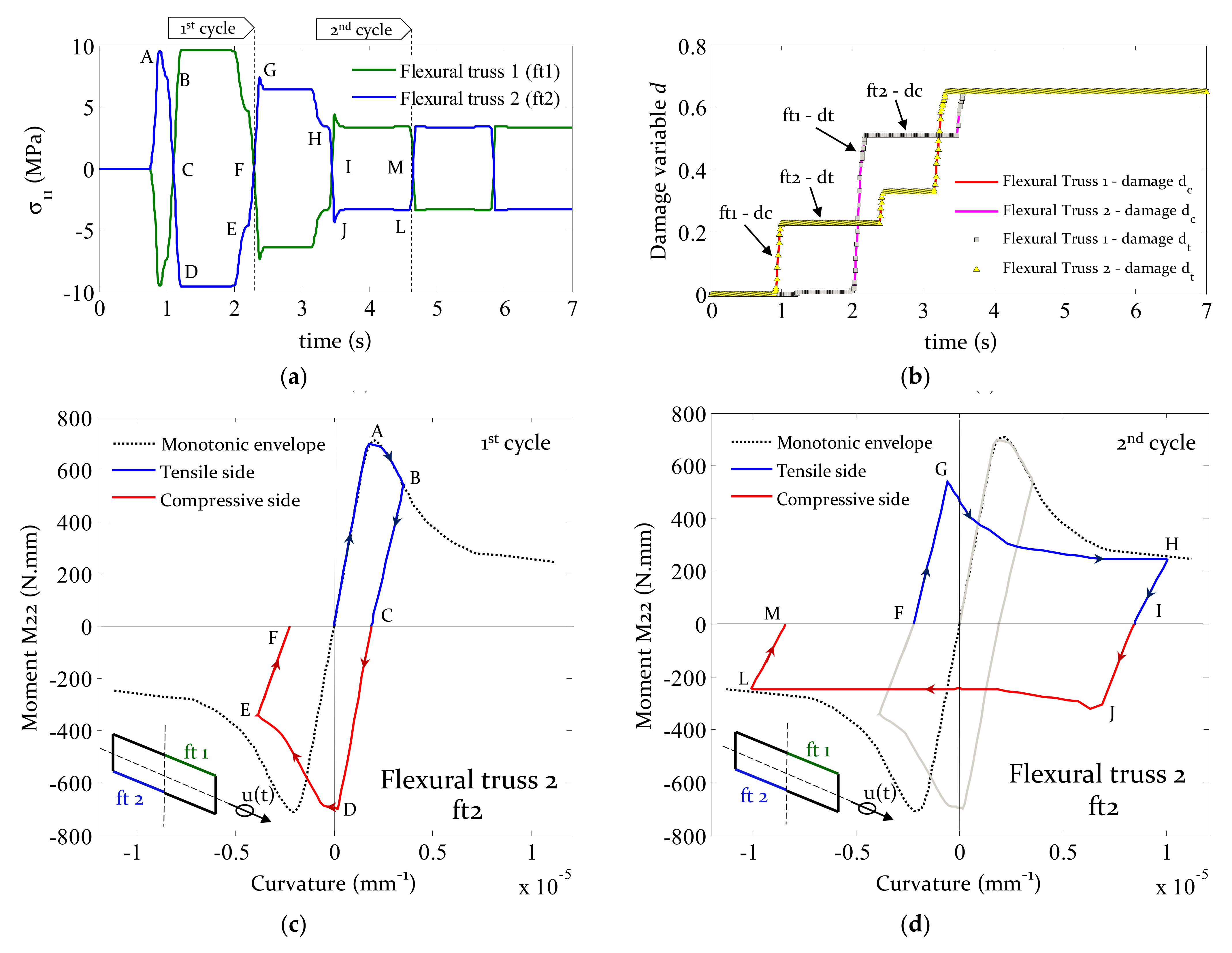
3.2.3. Bi–Directional Cyclic Loading

The last test covers the bi–directional cyclic loading response of the outlined case study in Figure 7. The goal is to see if the expected hysteretic behaviour of the flexural trusses is well reproduced. Both positive and negative vertical bending capacities are similar, hence both the flexural trusses, ft1 and ft2, need to trace the same behaviour. This was sustained by Figure 4 wherein the axial Cauchy stress ${\sigma }_{11}$ faced in both flexural trusses are similar in magnitude and, owing to the binary of the bending force, have an opposite signal.

Regarding the hysteretic behaviour, after completion of the first cycle (A$\to$F, $t=2.25s$), as depicted in Figure 11c, the tensile peak is reached at A and the first tensile unloading branch initiates at B with a stiffness given by $E_B=\left(1-d_t^B\right)E_0$ until C. The first compressive re–loading branch starts at C with a stiffness $E_0$, since a value of 1 has been defined for the recovery parameter ${\omega }_c$ and so, predictably, the maximum compressive stress at D reaches the same magnitude as A, i.e., the maximum quasi–static envelope. In the same manner, the unloading branch (E$\to$F) has a stiffness given by $\left(1-d_c^E\right)E_0$, and the first re–loading tensile branch (F$\to$G) has the same stiffness as the last unloading tensile branch (B$\to$C). This is equivalent for the first reloading compressive regime I$\to$J, which follows the same path as the last unloading phase E$\to$F. It is also noticeable that H and L have the same (in magnitude) axial stress ${\sigma }_{11}$ as the last point of the quasi–static envelope. The material constitutive behaviour formulation defines minimum stress, or the designated residual strength, to be the last effective stress given as input, see Figure 11. Thus, after reaching point H, the damage parameter remains stationary (Figure 11b).

It has been demonstrated that the cyclic behaviour is reproduced as it was expected. Both positive and negative vertical bending moments are represented (truss ft1 and ft2). It may be highlighted, again, that the latter holds true because total recovery effects have been defined for tensile and compressive regimes (${\omega }_t=1$ and ${\omega }_c=1$). Furthermore, the model exhibits the capacity of allocating in memory the damage variables, for both the preceding tensile and compressive cycle of each flexural trusses, allowing thus the calculation of the onward un(re)–loading cycle.

4. Computational Features and CPU Parallelisation

The implementation of the discrete model can be achieved using any FE–based platform. Nonetheless, the authors raise the importance of several modelling assumptions in the ease of such a process and for the optimisation of the associated computational costs. For instance, the importance of considering a node renumbering algorithm is presented next, together with the use of an implicit solver rather than an explicit one. At last, a comparison over the CPU time is performed between a traditional continuous FE model (smeared crack model) and the macro–element (discrete) model.

4.1. Node Renumbering Algorithm

A remark on the importance of adequate node renumbering is briefly stated hereafter. Its importance is evaluated in terms of time costs and required RAM to complete a linear elastic analysis. Such costs are influenced by the bandwidth dimension of the global stiffness matrix [K]. The minimisation of the latter through sparse matrices is well–documented [103,104] and several algorithms have been developed [105,106,107,108]. A brief test is performed on a masonry wall subjected to an out–of–plane surface load. Results are found for linear elastic analysis and through a direct sparse solver. A refined mesh of $35\times 65$ rigid quadrilateral elements represent the masonry wall. Two algorithms have been employed: (i) a geometric–based algorithm, in which mesh nodes are numbered according to a defined direction vector (length with higher dimension); and (ii) the so–called Approximate Minimum Degree (AMD) sparsity algorithm, in which the number of non–zero entries in the global stiffness matrix is reduced through a heuristic approach [109]. Results gathered in

Table 3. Performance test on an out–of–plane loaded masonry wall ($35\times 65$ elements) for two–node renumbering algorithms and within a direct sparse solver.

Node Renumbering Algorithm	None (Reference)	Geometric Algorithm	AMD Algorithm
CPU total time (s)	14.95	5.523 ($-$63.1%)	6.006 ($-59.8$%)
Optimum physical memory RAM (Mbytes)	137.1	69.93 ($-49$.0%)	76.23 ($-44$.4%)

were found through a 64–bit Windows 10 computer with 16 Gb RAM and Intel i7 CPU running at 3.4 GHz.

Although the absolute computational time difference may be negligible for the present benchmark, the use of an algorithm may reduce the relative CPU time by around 60% and around 44–49% of the required optimum physical memory. Such differences could be more relevant within a nonlinear quasi–static analysis since several steps (and iterations) need to be solved. Exploring the issue of the most efficient algorithm available in the literature is especially convenient for very large–scale structures, in which powerful pre–processors software as ANSA [110] can be used. Here, even if the performed test is simple, it aims to raise the awareness (or the discrete–model FE user) over the importance of a renumbering strategy. To cope with the concern of improving computational efficiency, ABAQUS offers a renumbering algorithm based on a geometrical method. This seems suitable for the dimension of the structural problems involved in the present study and in cases where a dominant length direction exists.

4.2. Implicit vs. Explicit FE Analysis

For dynamic analysis, the macro–system equilibrium can be solved using an implicit or explicit scheme. Still, two main reasons support the selection of an implicit procedure. The first concerns the modelling of the inertial mass system that is achieved by assigning a representative density value for the rigid plates only. In opposition, an explicit solver demands the insertion of density values for all the elements, which compromise the stability and representativeness of eigenvalues problems due to the local modal effects (associated with FE trusses). The second reason is linked to the intrinsic nature of each procedure. The explicit solver suffers from a time–step solution bias since considerable small–time increments are required to avoid a system misrepresentation. Although its use is recommended for many problems due to its stability—as fast–dynamic problems or when interface contact exists [111,112,113,114]—, an explicit solver may lead to long and prohibitive processing times and to larger disk storage space when conducting a seismic assessment study of a masonry structure. In converse, an implicit procedure allows larger time increments with the setback that a converged solution must be found for each iteration; however, this is well handled by the macro–element due to its robustness, as is demonstrated next in Section 4.3.

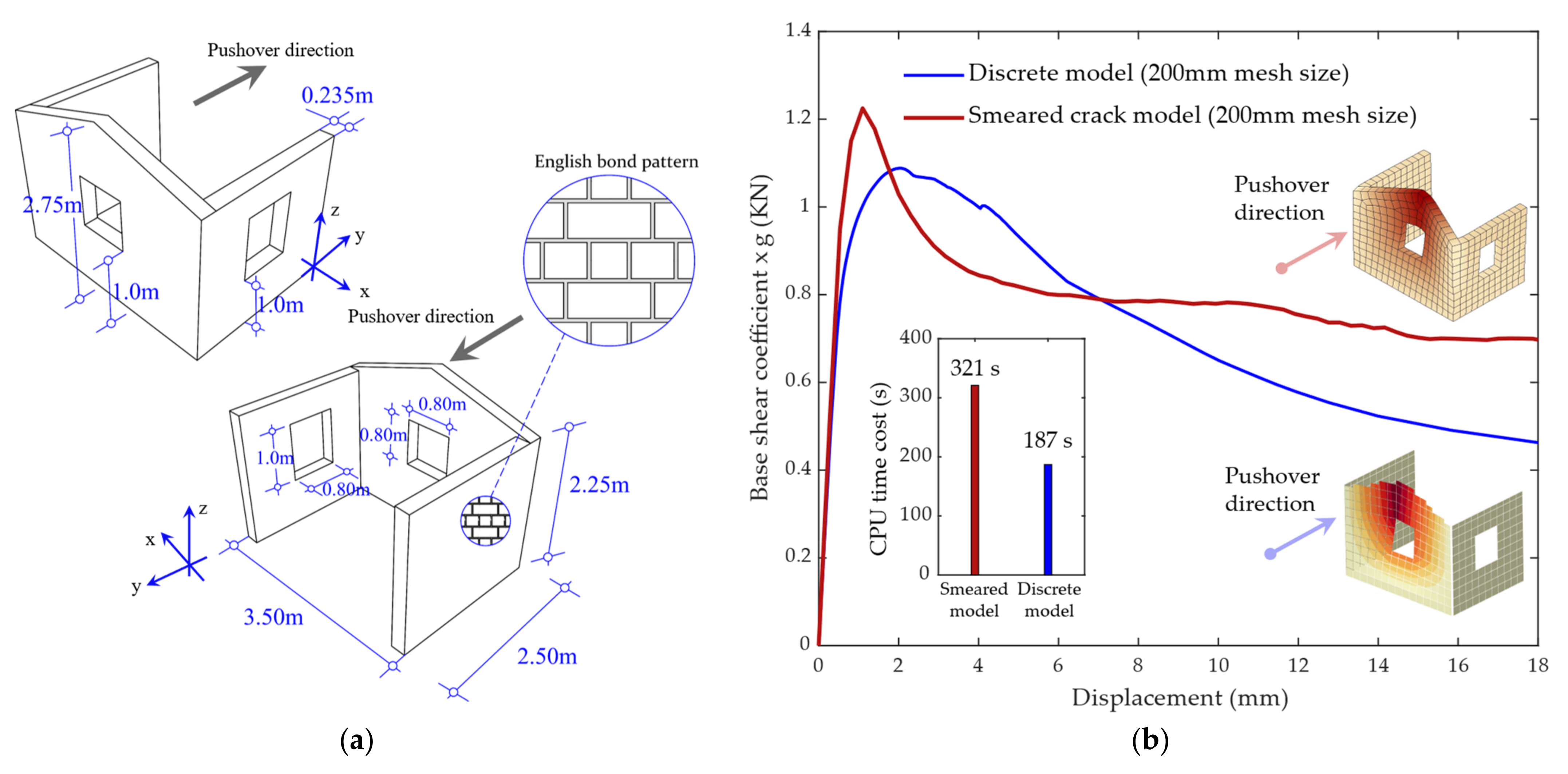
4.3. Comment on the Computational Attractiveness of the (Discrete) Macro–Element

It has been seen that the macro–scale behaviour arises from the deformation of in– and out–of–plane FE trusses that carry the material information (from experimentation or numerical homogenisation). Restricting the macro–deformation to linear elements brings direct advantages due to its simplicity and one–dimensionality of the constitutive equations, cyclic behaviour, strength domain, inelastic strain evolution laws, and damage evolution and tracking (closure–opening crack states). The use of advanced structural analysis software, such as ABAQUS, is of utmost importance. In cases where a given instability renders a not purely positive definite stiffness matrix, the traditional equation solvers (as the Newton–Raphson, the modified Newton–Raphson, or secant methods) are unable to give an adequate solution. In such situations, the software is robust because a modified Riks method ([115,116,117,118]) is at its disposal to overcome snap–back and snap–through issues. This is especially important when conducting quasi–static analysis in which material (and of other kinds) non–linearities are active. A quasi–static type of analysis is performed on the so–called LNEC brick house benchmark to demonstrate the efficiency of the macro–element. Figure 12a depicts the brick structure, which is composed of three walls in a U–shaped plan arrangement. The main façade presents a gable wall (dimensions 3.50 × 2.75 m²) and is linked with two transversal walls (dimensions 2.50 × 2.25 m²). Walls are constructed with clay brickwork in an English–bond arrangement and have 235 mm of thickness.

A mass proportional pushover analysis has been performed following the load direction indicated in Figure 12a. Results from the macro–element (discrete) are compared against a smeared (fixed) crack FE model. The assumed material properties (see

Table 4. Material properties adopted for the LNEC brick house benchmark performance test.

	Material Properties
	Exx (MPa)	Eyy (MPa)	$\mathit{\upsilon }$ (–)	ft (MPa)	Gftension (N/mm)	fc (MPa)	Gfcompression (N/mm)	fshear (MPa)	Gfshear (N/mm)
Macro–element (discrete) model	6400	3600	0.200	0.105	0.012	2.480	3.970	0.20	0.50
Smeared crack model	5170	5170						–	–

) are based on experimental and literature evidence [75,119], specifically the tension (f_t), compression (f_c), and shear (f_shear) strength values, and corresponding fracture energy terms. A mesh size equal to 200mm has been assumed for both models to guarantee the objectivity of the comparison. Likewise, the following have been considered (see [4]): (i) an exponential softening in tension [4] governed by the tensile fracture energy, Gf_tension; and (ii) a parabolic softening in compression [4] governed by the compressive fracture energy, Gf_compression. An exponential softening has been also assumed for the shear regime within the macro–element model, albeit it is disregarded for the smeared crack model.

Analyses have been computed on a 64–bit Windows 7 computer with 16 GB RAM and Intel i7 CPU running at 3.4 GHz. The obtained capacity curves and the required computational times are given in Figure 12b. Differences in the peak (around 12%) and post–peak response were expected due to the differences that both formulations contain. Nonetheless, the aim of this comparison resorts especially on the computational time rather than on the capacity curves. Herein, the macro–element allows reducing the computational cost by 41%. This is especially relevant if one states that the FE smeared crack models are typically the option for large–scale structures due to computational attractiveness [2,4,5]. The improvement in the CPU time is mainly associated with the lower number of iterations required by the macro–element model to compute the non–linear solution.

At last, the CPU time can be optimised if parallel computing is considered. In the present study, the authors do not claim any inherent advantages due to the small–scale of the structure. Nevertheless, parallelisation may have a special interest to speed up the processing times for dynamic or large–scale problems [120,121]. Likewise, the use of graphical processing units (GPU) can be an important booster, yet no investigation has been conducted in this regard. Still, the use of CPU parallelisation and GPU are always dependent on the machine at disposal

5. Final Remarks

A formal description and validation of a macro–element has been presented for the three–dimensional analysis of masonry structures. The macro–element is based on the FE method, but several simplifications have been developed to supply faster results than conventional continuous FE models, such as those retrieved from smeared crack approaches. It is aimed for the macro–scale analysis of structures, and based on a discrete approach; specifically, quadrilateral rigid plates are connected at its interfaces by a set of FE trusses. These one–dimensional elements govern the in–plane and out–of–plane deformations. The constitutive response can be based on any plasticity model; however, the so–called concrete damage plasticity model was assumed as it can reproduce well homogenised material data provided from experimentation or numerical homogenisation of concrete-like materials. A regularisation step corrects the fracture energy of the stress–strain input curves according to the defined macro–mesh dimensions, thus guaranteeing the well–posedness of the solution.

Validation and convergence tests have been performed to evaluate if the macro–element fulfils the requirements for (i) elastic problems; (ii) eigenvalue problems; and (iii) nonlinear problems for monotonic and cyclic loading cases. The tests have shown that the discrete model provides good results in both static and dynamic ranges. Likewise, it has been concluded that a refinement level given by L/15 (L is the length of the wall side being meshed) seems a reasonable choice for the mesh size when performing a structural analysis; at least in the case that a mesh sensitivity test is disregarded. Computational recommendations have been also briefly addressed, as the use of an implicit solver scheme, the use of the arc–length method for nonlinear quasi–static tests, and the use of a FE node renumbering algorithm.

Although the application of discrete systems may be questionable in cases where multiphase couplings can occur, as when thermal or hydro–mechanical effects exist, the latter macro–element proved to be suitable for structural–oriented problems such as the broader range of quasi–static and the seismic assessment of masonry structures. A decoupled characterisation for the admissible in– and out–of–plane deformations—that is certainly an approximation—proved to be reliable (at least for levels of pre–compression lower than the masonry compressive strength). Nonetheless, the macro–element is robust and can be implemented in any FE software, to any structural application, and perhaps more importantly, to be used by both professionals and academics. As future research streamlines, one can state that the reduced computational cost of the macro–element can be explored: (a) within larger–scale structures [122,123]; (b) within a structural health monitoring system [124,125] following the so–called digital twin framework; and (c) it can be accounted within a probabilistic–based features for reliability and robustness–based analysis.

References

1. Giamundo, V.; Sarhosis, V.; Lignola, G.P.; Sheng, Y.; Manfredi, G. Evaluation of different computational modelling strategies for the analysis of low strength masonry structures. Eng. Struct. 2014, 73, 160–169. [Google Scholar] [CrossRef] [Green Version]
2. de Felice, G.; De Santis, S.; Lourenço, P.B.; Mendes, N. Methods and Challenges for the Seismic Assessment of Historic Masonry Structures. Int. J. Archit. Herit. 2017, 11, 143–160. [Google Scholar] [CrossRef] [Green Version]
3. Sacco, E.; Addessi, D.; Sab, K. New trends in mechanics of masonry. Meccanica 2018, 53, 1565–1569. [Google Scholar] [CrossRef] [Green Version]
4. Lourenço, P.B.; Silva, L.C. Computational applications in masonry structures: From the meso–scale to the super-large/super-complex. Int. J. Multiscale Comput. Eng. 2020, 18, 1–30. [Google Scholar] [CrossRef]
5. Roca, P.; Cervera, M.; Gariup, G.; Pela’, L. Structural Analysis of Masonry Historical Constructions. Classical and Advanced Approaches. Arch. Comput. Methods Eng. 2010, 17, 299–325. [Google Scholar] [CrossRef] [Green Version]
6. Theodossopoulos, D.; Sinha, B. A review of analytical methods in the current design processes and assessment of performance of masonry structures. Constr. Build. Mater. 2013, 41, 990–1001. [Google Scholar] [CrossRef]
7. Tomaževič, M. Earthquake-Resistant Design of Masonry Buildings; World Scientific: London, UK, 1999; Volume 1. [Google Scholar]
8. Lagomarsino, S.; Penna, A.; Galasco, A.; Cattari, S. TREMURI program: An equivalent frame model for the nonlinear seismic analysis of masonry buildings. Eng. Struct. 2013, 56, 1787–1799. [Google Scholar] [CrossRef]
9. Quagliarini, E.; Maracchini, G.; Clementi, F. Uses and limits of the Equivalent Frame Model on existing unreinforced masonry buildings for assessing their seismic risk: A review. J. Build. Eng. 2017, 10, 166–182. [Google Scholar] [CrossRef]
10. Addessi, D.; Liberatore, D.; Masiani, R. Force-Based Beam Finite Element (FE) for the Pushover Analysis of Masonry Buildings. Int. J. Archit. Herit. 2015, 9, 231–243. [Google Scholar] [CrossRef]
11. Brencich, A.; Lagomarsino, S. A macroelement dynamic model for masonry shear walls. Comput. Methods Struct. Mason. 1998, 4, 67–75. [Google Scholar]
12. Penna, A.; Lagomarsino, S.; Galasco, A. A nonlinear macroelement model for the seismic analysis of masonry buildings. Earthq. Eng. Struct. Dyn. 2014, 43, 159–179. [Google Scholar] [CrossRef]
13. Vanin, F.; Penna, A.; Beyer, K. A three-dimensional macroelement for modelling the in-plane and out-of-plane response of masonry walls. Earthq. Eng. Struct. Dyn. 2020, 49, 1365–1387. [Google Scholar] [CrossRef]
14. Sangirardi, M.; Liberatore, D.; Addessi, D. Equivalent Frame Modelling of Masonry Walls Based on Plasticity and Damage. Int. J. Archit. Herit. 2019, 13, 1098–1109. [Google Scholar] [CrossRef]
15. Liberatore, D.; Addessi, D. Strength domains and return algorithm for the lumped plasticity equivalent frame model of masonry structures. Eng. Struct. 2015, 91, 167–181. [Google Scholar] [CrossRef]
16. D’Ayala, D.; Shi, Y. Modelling Masonry Historic Buildings by Multi-Body Dynamics. Int. J. Archit. Herit. 2011, 5, 483–512. [Google Scholar] [CrossRef]
17. Konstantinidis, D.; Makris, N. The dynamics of a rocking block in three dimensions. In Proceedings of the 8th HSTAM International Congress on Mechanics Mech, Patras, Greece, 12–14 July 2007; pp. 12–14. [Google Scholar]
18. D’Ayala, D.; Speranza, E. Definition of Collapse Mechanisms and Seismic Vulnerability of Historic Masonry Buildings. Earthq. Spectra 2003, 19, 479–509. [Google Scholar] [CrossRef]
19. Griffith, M.; Magenes, G. Evaluation of out-of-plane stability of unreinforced masonry walls subjected to seismic excitation. J. Earthq. Eng. 2003, 7, 141–169. [Google Scholar] [CrossRef]
20. Calvi, G.M.; Pinho, R.; Magenes, G.; Bommer, J.J.; Restrepo-Vélez, L.F.; Crowley, H. Development of seismic vulnerability assessment methodologies over the past 30 years. ISET J. Eathquake Technol. 2006, 43, 75–104. [Google Scholar]
21. Funari, M.F.; Mehrotra, A.; Lourenço, P.B. A tool for the rapid seismic assessment of historic masonry structures based on limit analysis optimisation and rocking dynamics. Appl. Sci. 2021, 11, 942. [Google Scholar] [CrossRef]
22. Funari, M.F.; Spadea, S.; Lonetti, P.; Fabbrocino, F.; Luciano, R. Visual programming for structural assessment of out-of-plane mechanisms in historic masonry structures. J. Build. Eng. 2020, 31, 101425. [Google Scholar] [CrossRef]
23. Baraldi, D.; Reccia, E.; Cecchi, A. In plane loaded masonry walls: DEM and FEM/DEM models. A critical review. Meccanica 2018, 53, 1613–1628. [Google Scholar] [CrossRef] [Green Version]
24. Cundall, P.; Hart, P. A computer model for simulating progressive large scale movements in blocky rock systems. Int. Soc. Rock Mech. (ISRM) 1971, 1, 28. [Google Scholar]
25. Shi, G.H.; Goodman, R.E. Discontinuous deformation analysis—A new method forcomputing stress, strain and sliding of block systems. In Proceedings of the 29th U.S. Symposium on Rock Mechanics (USRMS), Minneapolis, MN, USA, 13–15 June 1988. [Google Scholar]
26. Lemos, J.V. Discrete Element Modelling of Masonry Structures. Int. J. Archit. Herit. 2007, 1, 190–213. [Google Scholar] [CrossRef]
27. Gilbert, M.; Melbourne, C. Rigid-Block Analysis of Masonry Structures; Institution of Structural Engineers: London, UK, 1994; Volume 72. [Google Scholar]
28. Baggio, C.; Trovalusci, P. Stone assemblies under in-plane actions. Comparison between nonlinear discrete approaches. Comput Methods Struct. Mason. 1995, 3, 184–193. [Google Scholar]
29. Sarhosis, V.; Bagi, K.; Lemos, J.V.; Milani, G. (Eds.) Computational Modelling of Masonry Structures Using the Discrete Element Method; IGI Global: Hershey, PA, USA, 2016; ISBN 1522502319. [Google Scholar]
30. Schlegel, R.; Rautenstrauch, K. Failure analysis of masonry shear walls. In Numererical Modeling of Discrete Materials; Taylor and Francis Group: London, UK, 2004; pp. 15–18. [Google Scholar]
31. Lemos, J.; Costa, A.; Bretas, E. Assessment of the seismic capacity of stone masonry walls with block models. In Computational Methods in Earthquake Engineering; Springer: Dordrecht, The Netherlands, 2011; pp. 221–235. [Google Scholar]
32. Malomo, D.; DeJong, M.J. A Macro-Distinct Element Model (M-DEM) for out-of-plane analysis of unreinforced masonry structures. Eng. Struct. 2021, 244, 112754. [Google Scholar] [CrossRef]
33. Pulatsu, B.; Erdogmus, E.; Lourenço, P.B.; Lemos, J.V.; Tuncay, K. Simulation of the in-plane structural behaviour of unreinforced masonry walls and buildings using DEM. Structures 2020, 27, 2274–2287. [Google Scholar] [CrossRef]
34. Peña, F.; Prieto, F.; Lourenço, P.B.; Costa, A.C.; Lemos, J.V. On the dynamics of rocking motion of single rigid–block structures. Earthq. Eng. Struct. Dyn. 2007, 36, 2383–2399. [Google Scholar] [CrossRef] [Green Version]
35. Itasca UDEC—Universal Distinct Element Code; Itasca Consulting Group Inc.: Minneapolis, MN, USA, 2004.
36. Cascini, L.; Gagliardo, R.; Portioli, F. LiABlock_3D: A Software Tool for Collapse Mechanism Analysis of Historic Masonry Structures. Int. J. Archit. Herit. 2018, 14, 75–94. [Google Scholar] [CrossRef]
37. Giambanco, G.; Rizzo, S.; Spallino, R. Numerical analysis of masonry structures via interface models. Comput. Methods Appl. Mech. Eng. 2001, 190, 6493–6511. [Google Scholar] [CrossRef]
38. Macorini, L.; Izzuddin, B.A. A non-linear interface element for 3D mesoscale analysis of brick-masonry structures. Int. J. Numer. Methods Eng. 2011, 85, 1584–1608. [Google Scholar] [CrossRef] [Green Version]
39. Lotfi, H.R.; Shing, P.B. Interface Model Applied to Fracture of Masonry Structures. J. Struct. Eng. 1994, 120, 63–80. [Google Scholar] [CrossRef]
40. Macorini, L.; Izzuddin, B.A. Nonlinear analysis of masonry structures using mesoscale partitioned modelling. Adv. Eng. Softw. 2013, 60–61, 58–69. [Google Scholar] [CrossRef]
41. Sejnoha, J.; Sejnoha, M.; Zeman, J.; Sykora, J.; Vorel, J. A mesoscopic study on historic masonry. Struct. Eng. Mech. 2008, 30, 99–117. [Google Scholar] [CrossRef]
42. Sarhosis, V.; Tsavdaridis, K.; Giannopoulos, I. Discrete Element Modelling (DEM) for Masonry Infilled Steel Frames with Multiple Window Openings Subjected to Lateral Load Variations. Open Constr. Build. Technol. J. 2014, 8, 93–103. [Google Scholar] [CrossRef]
43. Adam, J.M.; Brencich, A.; Hughes, T.G.; Jefferson, T. Micromodelling of eccentrically loaded brickwork: Study of masonry wallettes. Eng. Struct. 2010, 32, 1244–1251. [Google Scholar] [CrossRef]
44. Dauda, J.A.; Silva, L.C.; Lourenço, P.B.; Iuorio, O. Out-of-plane loaded masonry walls retrofitted with oriented strand boards: Numerical analysis and influencing parameters. Eng. Struct. 2021, 243, 112683. [Google Scholar] [CrossRef]
45. Silva, L.C.; Lourenço, P.B.; Milani, G. Derivation of the out-of-plane behaviour of masonry through homogenization strategies: Micro-scale level. Comput. Struct. 2018, 209, 30–43. [Google Scholar] [CrossRef]
46. Aşıkoğlu, A.; Avşar, Ö.; Lourenço, P.B.; Silva, L.C. Effectiveness of seismic retrofitting of a historical masonry structure: Kütahya Kurşunlu Mosque, Turkey. Bull. Earthq. Eng. 2019, 17, 3365–3395. [Google Scholar] [CrossRef]
47. Ciocci, M.P.; Sharma, S.; Lourenço, P.B. Engineering simulations of a super-complex cultural heritage building: Ica Cathedral in Peru. Meccanica 2018, 53, 1931–1958. [Google Scholar] [CrossRef]
48. Reccia, E.; Leonetti, L.; Trovalusci, P.; Cecchi, A. A multiscale/multidomain model for the failure analysis of masonry walls: A validation with a combined FEM/DEM approach. Int. J. Multiscale Comput. Eng. 2018, 16, 325–343. [Google Scholar] [CrossRef]
49. Tiberti, S.; Milani, G. 2D pixel homogenized limit analysis of non-periodic masonry walls. Comput. Struct. 2019, 219. [Google Scholar] [CrossRef]
50. Trovalusci, P.; Ostoja-Starzewski, M.; De Bellis, M.L.; Murrali, A. Scale-dependent homogenization of random composites as micropolar continua. Eur. J. Mech.—A/Solids 2015, 49, 396–407. [Google Scholar] [CrossRef]
51. Addessi, D.; Sacco, E.; Paolone, A. Cosserat model for periodic masonry deduced by nonlinear homogenization. Eur. J. Mech—A/Solids 2010, 29, 724–737. [Google Scholar] [CrossRef]
52. Šejnoha, M.; Janda, T.; Vorel, J.; Kucíková, L.; Padevěd, P. Combining Homogenization, Indentation and Bayesian Inference in Estimating the Microfibril Angle of Spruce. Procedia Eng. 2017, 190, 310–317. [Google Scholar] [CrossRef]
53. Otero, F.; Oller, S.; Martinez, X.; Salomón, O. Numerical homogenization for composite materials analysis. Comparison with other micro mechanical formulations. Compos. Struct. 2015, 122, 405–416. [Google Scholar] [CrossRef] [Green Version]
54. Driesen, C.; Degée, H.; Vandoren, B. Efficient modelling of masonry failure using a multiscale domain activation approach. Comput. Struct. 2021, 251, 106543. [Google Scholar] [CrossRef]
55. Funari, M.F.; Silva, L.C.; Savalle, N.; Lourenço, P.B. A concurrent micro/macro FE-model optimized with a limit analysis tool for the assessment of dry-joint masonry structures. Int. J. Multiscale Comput. Eng. 2022. [Google Scholar] [CrossRef]
56. Maria D’Altri, A.; Lo Presti, N.; Grillanda, N.; Castellazzi, G.; de Miranda, S.; Milani, G. A two-step automated procedure based on adaptive limit and pushover analyses for the seismic assessment of masonry structures. Comput. Struct. 2021, 252, 106561. [Google Scholar] [CrossRef]
57. Mistler, M.; Anthoine, A.; Butenweg, C. In-plane and out-of-plane homogenisation of masonry. Comput. Struct. 2007, 85, 1321–1330. [Google Scholar] [CrossRef]
58. Barenblatt, G.I. The formation of equilibrium cracks during brittle fracture. General ideas and hypotheses. Axially-symmetric cracks. J. Appl. Math. Mech. 1959, 23, 622–636. [Google Scholar] [CrossRef]
59. Xu, X.-P.; Needleman, A. Numerical simulations of fast crack growth in brittle solids. J. Mech. Phys. Solids 1994, 42, 1397–1434. [Google Scholar] [CrossRef]
60. Belytschko, T.; Moës, N.; Usui, S.; Parimi, C. Arbitrary discontinuities in finite elements. Int. J. Numer. Methods Eng. 2001, 50, 993–1013. [Google Scholar] [CrossRef] [Green Version]
61. De Borst, R. Computation of post-bifurcation and post-failure behaviour of strain-softening solids. Comput. Struct. 1987, 25, 211–224. [Google Scholar] [CrossRef] [Green Version]
62. Lourenço, P.B.; De Borst, R.; Rots, J.G. A plane stress softening plasticity model for orthotropic materials. Int. J. Numer. Methods Eng. 1997, 40, 4033–4057. [Google Scholar] [CrossRef]
63. de Borst, R. Fracture in quasi-brittle materials: A review of continuum damage-based approaches. Eng. Fract. Mech. 2002, 69, 95–112. [Google Scholar] [CrossRef]
64. Clemente, R.; Roca, P.; Cervera, M. Damage model with crack localization—Application to historical buildings. In Proceedings of the Structural Analysis of Historical Constructions, New Delhi, India, 6–8 November 2006; Lourenço, P.B., Roca, P., Modena, C., Agrawal, S., Eds.; Macmillan Publishers India Limited: Lucknow, India, 2006; pp. 1125–1134. [Google Scholar]
65. Wu, J.-Y.; Cervera, M. A thermodynamically consistent plastic-damage framework for localized failure in quasi-brittle solids: Material model and strain localization analysis. Int. J. Solids Struct. 2016, 88–89, 227–247. [Google Scholar] [CrossRef]
66. Milani, G.; Lourenço, P.B.; Tralli, A. Homogenised limit analysis of masonry walls, Part II: Structural examples. Comput. Struct. 2006, 84, 181–195. [Google Scholar] [CrossRef] [Green Version]
67. Milani, G.; Tralli, A. Simple SQP approach for out-of-plane loaded homogenized brickwork panels, accounting for softening. Comput. Struct. 2011, 89, 201–215. [Google Scholar] [CrossRef]
68. Milani, G.; Venturini, G. Automatic fragility curve evaluation of masonry churches accounting for partial collapses by means of 3D FE homogenized limit analysis. Comput. Struct. 2011, 89, 1628–1648. [Google Scholar] [CrossRef]
69. Casolo, S. Macroscopic modelling of structured materials: Relationship between orthotropic Cosserat continuum and rigid elements. Int. J. Solids Struct. 2006, 43, 475–496. [Google Scholar] [CrossRef] [Green Version]
70. Casolo, S.; Milani, G. Simplified out-of-plane modelling of three-leaf masonry walls accounting for the material texture. Constr. Build. Mater. 2013, 40, 330–351. [Google Scholar] [CrossRef]
71. Scacco, J.; Ghiassi, B.; Milani, G.; Lourenço, P.B. A fast modelling approach for numerical analysis of unreinforced and FRCM reinforced masonry walls under out-of-plane loading. Compos. Part B Eng. 2020, 180, 107553. [Google Scholar] [CrossRef]
72. Scacco, J.; Milani, G.; Lourenço, P.B. Automatic mesh generator for the non-linear homogenized analysis of double curvature masonry structures. Adv. Eng. Softw. 2020, 150, 102919. [Google Scholar] [CrossRef]
73. Casolo, S. Rigid element model for non-linear analysis of masonry façades subjected to out-of-plane loading. Commun. Numer. Methods Eng. 1999, 15, 457–468. [Google Scholar] [CrossRef]
74. Silva, L.C.; Lourenço, P.B.; Milani, G. Rigid block and spring homogenized model (HRBSM) for masonry subjected to impact and blast loading. Int. J. Impact Eng. 2017, 109, 14–28. [Google Scholar] [CrossRef]
75. Silva, L.C.; Lourenço, P.B.; Milani, G. Numerical homogenization-based seismic assessment of an English-bond masonry prototype: Structural level application. Earthq. Eng. Struct. Dyn. 2020, 49, 841–862. [Google Scholar] [CrossRef]
76. Sharma, S.; Silva, L.C.; Graziotti, F.; Magenes, G.; Milani, G. Modelling the experimental seismic out-of-plane two-way bending response of unreinforced periodic masonry panels using a non-linear discrete homogenized strategy. Eng. Struct. 2021, 242, 112524. [Google Scholar] [CrossRef]
77. Uva, G.; Tateo, V.; Casolo, S. Presentation and validation of a specific RBSM approach for the meso-scale modelling of in-plane masonry-infills in RC frames. Int. J. Mason. Res. Innov. 2020, 5, 366–395. [Google Scholar] [CrossRef]
78. Silva, L.C.; Lourenço, P.B.; Milani, G. Nonlinear Discrete Homogenized Model for Out-of-Plane Loaded Masonry Walls. J. Struct. Eng. 2017, 143, 4017099. [Google Scholar] [CrossRef] [Green Version]
79. Kawai, T. New discrete structural models and generalization of the method of limit analysis. In Proceedings of the Finite Elements in Nonlinear Mechanics, Geilo, Norway, August 1977; Tapir Publishers: Trondheim, Norway, 1977; pp. 885–906. [Google Scholar]
80. Kawai, T. New discrete models and their application to seismic response analysis of structures. Nucl. Eng. Des. 1978, 48, 207–229. [Google Scholar] [CrossRef]
81. Kawai, T. Discrete limit analysis of reinforced concrete structures using rigid bodies-spring models. In The Finite Element Method In the 1990’s; Springer: Berlin/Heidelberg, Germany, 1991; pp. 182–191. [Google Scholar]
82. Kannan, R.; Hendry, S.; Higham, N.J.; Tisseur, F. Detecting the causes of ill-conditioning in structural finite element models. Comput. Struct. 2014, 133, 79–89. [Google Scholar] [CrossRef] [Green Version]
83. Bertolesi, E.; Silva, L.C.; Milani, G. Validation of a two-step simplified compatible homogenisation approach extended to out-plane loaded masonries. Int. J. Mason. Res. Innov. 2019, 4, 265. [Google Scholar] [CrossRef]
84. Bertolesi, E.; Milani, G.; Lourenço, P.B. Implementation and validation of a total displacement non-linear homogenization approach for in-plane loaded masonry. Comput. Struct. 2016, 176, 13–33. [Google Scholar] [CrossRef] [Green Version]
85. Lubliner, J.; Oliver, J.; Oller, S.; Oñate, E. A plastic-damage model for concrete. Int. J. Solids Struct. 1989, 25, 299–326. [Google Scholar] [CrossRef]
86. Lee, J.; Fenves, G.L. Plastic-Damage Model for Cyclic Loading of Concrete Structures. J. Eng. Mech. 1998, 124, 892–900. [Google Scholar] [CrossRef]
87. Grassl, P.; Jirásek, M. Damage-plastic model for concrete failure. Int. J. Solids Struct. 2006, 43, 7166–7196. [Google Scholar] [CrossRef] [Green Version]
88. Duvaut, G.; Lions, J.L. Les Inéquations En Mécanique et en Physique; Dunod: Paris, France, 1972. [Google Scholar]
89. Bažant, Z.P.; Oh, B.H. Crack band theory for fracture of concrete. Matériaux Constr. 1983, 16, 155–177. [Google Scholar] [CrossRef] [Green Version]
90. Bacigalupo, A.; Gambarotta, L.; Lepidi, M. Thermodynamically consistent non-local continualization for masonry-like systems. Int. J. Mech. Sci. 2021, 205, 106538. [Google Scholar] [CrossRef]
91. Addessi, D.; Sacco, E. Enriched plane state formulation for nonlinear homogenization of in-plane masonry wall. Meccanica 2016, 51, 2891–2907. [Google Scholar] [CrossRef]
92. Irons, B.M. Numerical integration applied to finite element methods. In Proceedings of the Conference on Use of Digital Computers in Structural Engineering; University of Newcastle: Newcastle, UK, 1966. [Google Scholar]
93. Irons, B.M.; Razzaque, A. Experience with the patch test for convergence of finite elements. In The Mathematical Foundations of the Finite Element Method with Applications to Partial Differential Equations; Academic Press: Cambridge, MA, USA, 1972; pp. 557–587. ISBN 978-0-12-068650-6. [Google Scholar]
94. Irons, B.; Loikkanen, M. An engineers’ defence of the patch test. Int. J. Numer. Methods Eng. 1983, 19, 1391–1401. [Google Scholar] [CrossRef]
95. Macneal, R.H.; Harder, R.L. A proposed standard set of problems to test finite element accuracy. Finite Elem. Anal. Des. 1985, 1, 3–20. [Google Scholar] [CrossRef]
96. Zienkiewicz, O.C.; Zhu, J.Z. The superconvergent patch recovery (SPR) and adaptive finite element refinement. Comput. Methods Appl. Mech. Eng. 1992, 101, 207–224. [Google Scholar] [CrossRef]
97. Hughes, T.J.R.; Cottrell, J.A.; Bazilevs, Y. Isogeometric analysis: CAD, finite elements, NURBS, exact geometry and mesh refinement. Comput. Methods Appl. Mech. Eng. 2005, 194, 4135–4195. [Google Scholar] [CrossRef] [Green Version]
98. Taylor, R.L.; Simo, J.C.; Zienkiewicz, O.C.; Chan, A.C.H. The patch test—A condition for assessing FEM convergence. Int. J. Numer. Methods Eng. 2018, 22, 39–62. [Google Scholar] [CrossRef]
99. Rao, K.M.; Shrinivasa, U. A set of pathological tests to validate new finite elements. Sadhana 2001, 26, 549–590. [Google Scholar] [CrossRef] [Green Version]
100. Zienkiewicz, O.C.; Taylor, R.L. The Finite Element Method: Solid Mechanics; Butterworth-Heinemann: Oxford, UK, 2000; Volume 2, ISBN 0750650559. [Google Scholar]
101. Turco, E.; Caracciolo, P. Elasto-plastic analysis of Kirchhoff plates by high simplicity finite elements. Comput. Methods Appl. Mech. Eng. 2000, 190, 691–706. [Google Scholar] [CrossRef]
102. Navier, C.L.M.H. Extrait des recherches sur la flexion des plans elastiques. Bull. Sci. Soc. Philomarhique 1823, 5, 95–102. [Google Scholar]
103. Collins, R.J. Bandwidth reduction by automatic renumbering. Int. J. Numer. Methods Eng. 1973, 6, 345–356. [Google Scholar] [CrossRef]
104. Cuthill, E.; McKee, J. Reducing the bandwidth of sparse symmetric matrices. In Proceedings of the 1969 24th National Conference, New York, NY, USA, 26–28 August 1969; ACM: New York, NY, USA, 1969; pp. 157–172. [Google Scholar]
105. Bathe, K.-J.; Wilson, E.L. Solution methods for eigenvalue problems in structural mechanics. Int. J. Numer. Methods Eng. 1973, 6, 213–226. [Google Scholar] [CrossRef]
106. Bathe, K.J.; Wilson, E.L. NONSAP—A nonlinear structural analysis program. Nucl. Eng. Des. 1974, 29, 266–293. [Google Scholar] [CrossRef]
107. Mafteiu-Scai, L.O. The Bandwidths of a Matrix. A Survey of Algorithms. Ann. West Univ. Timisoara Math. Comput. Sci. 2014, 52, 183–223. [Google Scholar] [CrossRef] [Green Version]
108. Pop, P.; Matei, O.; Comes, C.-A. Reducing the bandwidth of a sparse matrix with a genetic algorithm. Optimization 2014, 63, 1851–1876. [Google Scholar] [CrossRef]
109. Amestoy, P.R.; Davis, T.A.; Duff, I.S. Algorithm 837: AMD, an Approximate Minimum Degree Ordering Algorithm. ACM Trans. Math. Softw. 2004, 30, 381–388. [Google Scholar] [CrossRef]
110. BETA CAE Systems International. ANSA The advanced CAE pre-processing software for complete model build up. In Proceedings of the OpenFOAM User Meeting Stammtisch United, Kassel, Germany, 20–21 February 2017; BETA CAE Systems International: Root, Switzerland, 2017. [Google Scholar]
111. Belytschko, T.; Lin, J.I.; Chen-Shyh, T. Explicit algorithms for the nonlinear dynamics of shells. Comput. Methods Appl. Mech. Eng. 1984, 42, 225–251. [Google Scholar] [CrossRef]
112. Burnett, S.; Gilbert, M.; Molyneaux, T.; Beattie, G.; Hobbs, B. The performance of unreinforced masonry walls subjected to low-velocity impacts: Finite element analysis. Int. J. Impact Eng. 2007, 34, 1433–1450. [Google Scholar] [CrossRef]
113. Hilber, H.M.; Hughes, T.J.R.; Taylor, R.L. Improved numerical dissipation for time integration algorithms in structural dynamics. Earthq. Eng. Struct. Dyn. 1977, 5, 283–292. [Google Scholar] [CrossRef] [Green Version]
114. Rafsanjani, S.H.; Lourenço, P.B.; Peixinho, N. Implementation and validation of a strain rate dependent anisotropic continuum model for masonry. Int. J. Mech. Sci. 2015, 104, 24–43. [Google Scholar] [CrossRef] [Green Version]
115. Riks, E. Some computational aspects of the stability analysis of nonlinear structures. Comput. Methods Appl. Mech. Eng. 1984, 47, 219–259. [Google Scholar] [CrossRef]
116. Riks, E. An incremental approach to the solution of snapping and buckling problems. Int. J. Solids Struct. 1979, 15, 529–551. [Google Scholar] [CrossRef]
117. Crisfield, M.A. A fast incremental/iterative solution procedure that handles “snap-through”. Comput. Struct. 1981, 13, 55–62. [Google Scholar] [CrossRef]
118. Powell, G.; Simons, J. Improved iteration strategy for nonlinear structures. Int. J. Numer. Methods Eng. 1981, 17, 1455–1467. [Google Scholar] [CrossRef]
119. Candeias, P.X.; Costa, A.C.; Mendes, N.; Costa, A.; Lourenço, P.B. Experimental Assessment of the Out-of-Plane Performance of Masonry Buildings Through Shaking Table Tests. Int. J. Archit. Herit. 2017, 11, 31–58. [Google Scholar] [CrossRef] [Green Version]
120. Kruis, J.; Krejčí, T.; Šejnoha, M. Parallel computing in multi-scale analysis of coupled heat and moisture transport in masonry structures. In High Performance Computing in Science and Engineering; Kozubek, T., Blaheta, R., Šístek, J., Rozložník, M., Čermák, M., Eds.; Springer International Publishing: Cham, Switzerland, 2016; pp. 50–59. [Google Scholar]
121. Krejčí, T.; Kruis, J.; Šejnoha, M.; Koudelka, T. Hybrid parallel approach to homogenization of transport processes in masonry. Adv. Eng. Softw. 2017, 113, 25–33. [Google Scholar] [CrossRef]
122. Fortunato, G.; Funari, M.F.; Lonetti, P. Survey and seismic vulnerability assessment of the Baptistery of San Giovanni in Tumba (Italy). J. Cult. Herit. 2017, 26, 64–78. [Google Scholar] [CrossRef]
123. Clementi, F.; Gazzani, V.; Poiani, M.; Lenci, S. Assessment of seismic behaviour of heritage masonry buildings using numerical modelling. J. Build. Eng. 2016, 8, 29–47. [Google Scholar] [CrossRef]
124. Barontini, A.; Masciotta, M.G.; Ramos, L.F.; Amado-Mendes, P.; Lourenço, P.B. An overview on nature-inspired optimization algorithms for Structural Health Monitoring of historical buildings. Procedia Eng. 2017, 199, 3320–3325. [Google Scholar] [CrossRef]
125. Funari, M.F.; Verre, S. The Effectiveness of the DIC as a Measurement System in SRG Shear Strengthened Reinforced Concrete Beams. Crystals 2021, 11, 265. [Google Scholar] [CrossRef]
Figure 1. Macro–unit cell and kinematics of the macro–element. (a) Out–of–plane. (b) In–plane.
Applsci 12 01248 g001
Figure 2. In–plane unit cell: a tributary area for each truss and kinematics of each allowable (admissible) deformation mode.
Applsci 12 01248 g002
Figure 3. Out–of–plane unit cell: the tributary area for each truss and kinematics of each allowable deformation mode.
Applsci 12 01248 g003
Figure 4. Hysteretic curve adopted for the out–of–plane trusses (note: for the in–plane truss beams, the tensile and compressive behaviours can have different shapes that stem from material characterisation).
Applsci 12 01248 g004
Figure 5. Convergence study conducted for a squared plate test.
Applsci 12 01248 g005
Figure 6. Deformed shape of the first eight eigenmodes obtained with the macro–element (discrete) model and through a classical FEA.
Applsci 12 01248 g006
Figure 7. Nonlinear validation of the macro–constitutive model for an out–of–plane loaded wall. (a) Vertical masonry wall. (b) Uni– and bi–directional cyclic loading.
Applsci 12 01248 g007
Figure 8. Procedure for integrating the homogenised vertical stress–strain curves on the masonry thickness aiming to obtain the homogenised vertical bending moment curve for the benchmark test.
Applsci 12 01248 g008
Figure 9. Quasi–static test: expected vs. obtained bending moment capacity curve.
Applsci 12 01248 g009
Figure 10. Uni–directional cyclic behaviour (Note: only the positive moments are plotted, i.e., the part of the unloading branch for negative bending moments has been disregarded for the sake of readiness).
Applsci 12 01248 g010
Figure 11. Bi–directional cyclic loading. (a) Cauchy stress σ 11 for flexural trusses. (b) Evolution of the damage parameter, d, for the flexural trusses. (c) Vertical bending moment–curvature (first cycle). (d) Vertical bending moment–curvature (second cycle).
Applsci 12 01248 g011
Figure 12. Capacity (pushover) curve and required CPU time for the LNEC house benchmark: comparison between the macro–element (discrete) model and smeared crack model. (a) Geometry of the LNEC brick house. (b) Capacity curves and required CPU time.
Applsci 12 01248 g012